A Machine Learning Approach for Classifying Road Accident Hotspots

Abstract

Road accidents are a worldwide problem, affecting millions of people annually. One way to reduce such accidents is to predict risk areas and alert drivers. Advanced research has been carried out on identifying accident-influencing factors and potential highway risk areas to mitigate the number of road accidents. Machine learning techniques have been used to build prediction models using a supervised classification based on a labeled dataset. In this work, we experimented with many machine learning algorithms to discover the best classifier for the Brazilian federal road hotspots associated with severe or nonsevere accident risk using several features. We tested with SVM, random forest, and a multi-layer perceptron neural network. The dataset contains a ten-year road accident report by the Brazilian Federal Highway Police. The feature set includes spatial footprint, weekday and time when the accident happened, road type, route, orientation, weather conditions, and accident type. The results were promising, and the neural network model provided the best results, achieving an accuracy of 83%, a precision of 84%, a recall of 83%, and an F1-score of 82%.

1. Introduction

Currently, road accidents are one of the world’s most critical problems, being a cause of concern and an object of study in many countries [1,2,3,4,5]. According to the World Health Organization (WHO), road accidents are the eighth leading cause of death in the world (https://www.who.int/violence_injury_prevention/road_safety_status/2018/en/, accessed on 30 January 2023), and Brazil has the fifth most violent traffic globally (https://apps.who.int/iris/bitstream/handle/10665/276462/9789241565684-eng.pdf?ua=1, accessed on 30 January 2023).

Since 2007, the Brazilian Federal Highway Police (PRF) has been collecting and publishing data on accidents that occurred on the federal highways. These data are available on the PRF website (https://portal.prf.gov.br, accessed on 30 January 2023), and it contains information on each accident, classified by year. From 2007 to 2017, they registered over 1.6 million accidents on Brazilian highways, where 83,498 people died, and over one million were injured. There are, on average, 23 deaths per day. 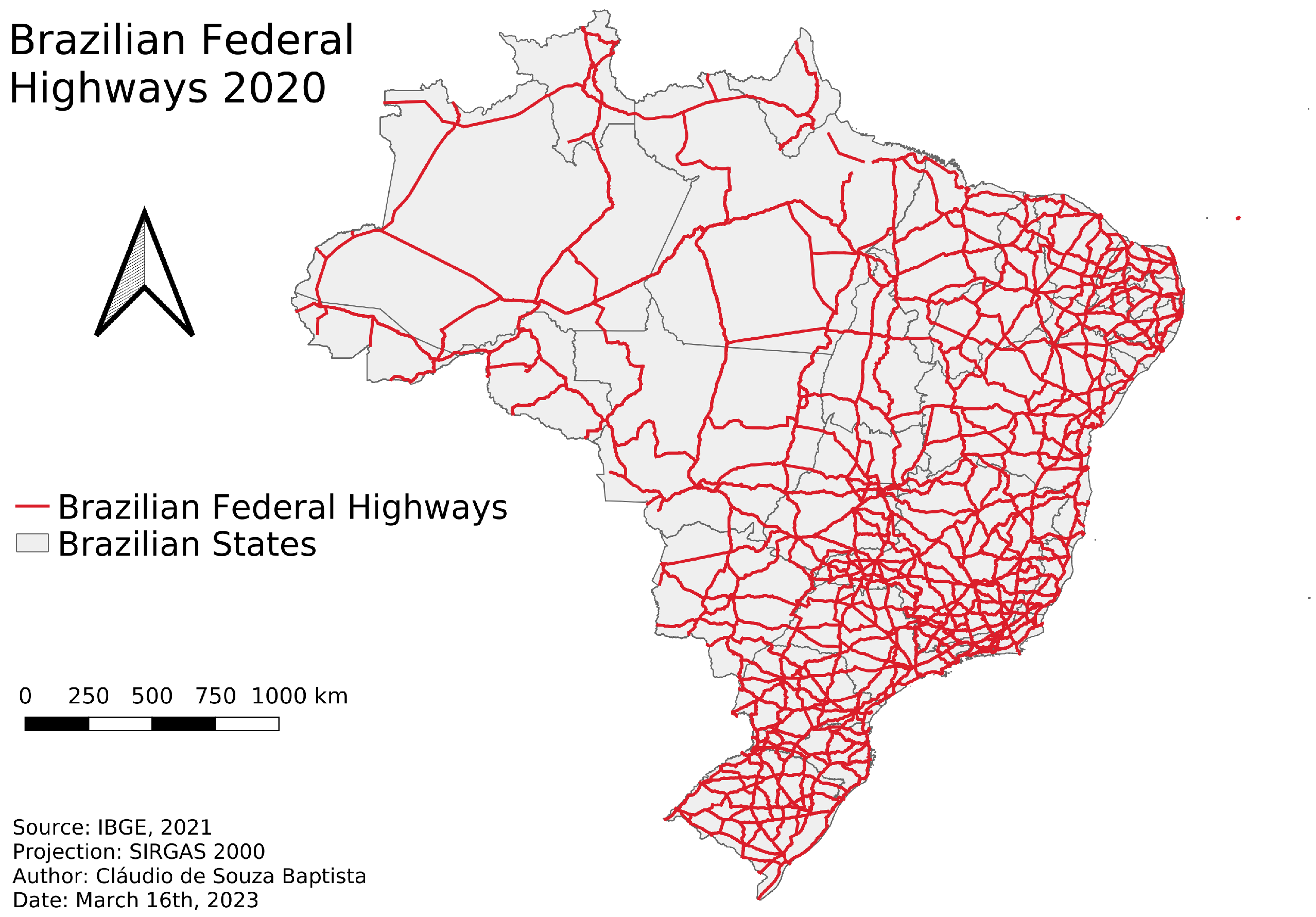Figure 1 depicts a map of the federal highways of Brazil. 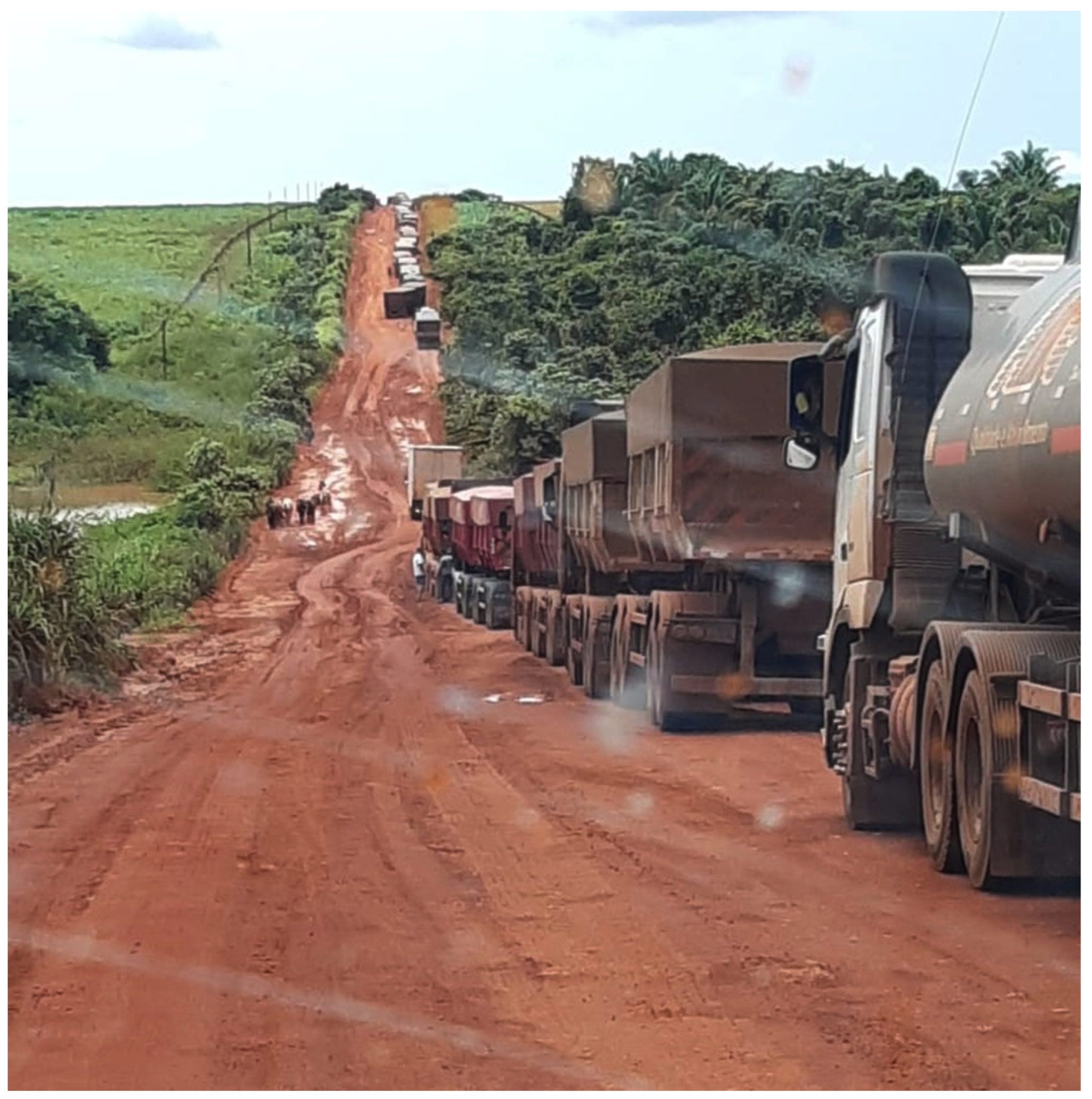In Figure 2, we observe an accident hotspot on BR-158, a highway with more accidents in Brazil. 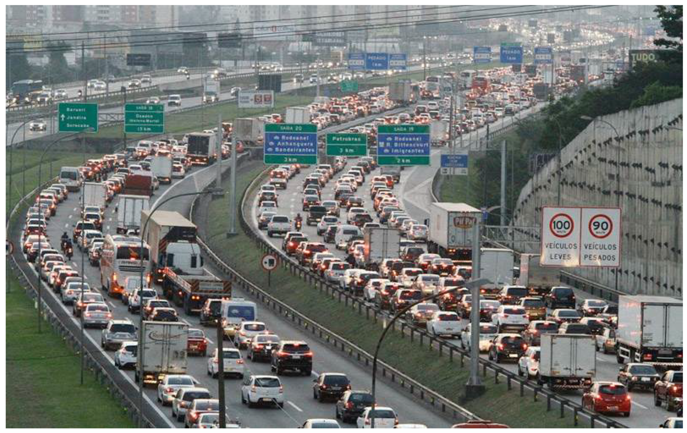Figure 3 shows the urban traffic in São Paulo, Brazil.

Several studies are addressing this problem since it does not affect only Brazil, making the accident data analysis field more popular [3,4,6,7]. The main objectives of these studies include understanding the risk factors contributing to accidents and creating measures to reduce such accidents.

Understanding the risk factors is crucial to predicting major accident features and reducing such road accidents. According to [1], the most frequent causes of accidents with young drivers are inexperience and excessive speed, while mental fatigue, physical handicap, and reduced cognitive and psychomotor capacity stand out with adult drivers. Accident risk factors have different impacts in different locations [8]. Therefore, analyzing new data on accidents will produce further information about the problems in a given locality.

Studies about machine learning models and road accidents are highly adaptable, with no or few assumptions about the input features. Machine learning approaches offer higher flexibility for outliers, inaccurate data, and missing data [9]. The main disadvantage of machine learning models is their performance as a “black box”, which leads to a fuzzy inference of the function that correlates the input variables with the target class [10]. Popular models applied to traffic accident-related studies include Decision Trees [11], Support Vector Machines (SVMs) [12], and Artificial Neural Networks (ANNs) [13].

This work proposes to build a machine-learning (ML)-based approach that allows us to classify and predict sections of highways that might be dangerous concerning the occurrence of accidents with vehicles. In addition, we present the application of the proposed method to Brazilian highways using a ten-year accident dataset recorded by the Federal Highway Police. The presented results aim to identify the best algorithms for predicting dangerous sections of Brazilian highways.

We will predict the danger in a highway section according to accidents that have occurred in the same area and are considered severe or nonsevere. Several factors were considered, such as the weather conditions, time of day in which the accident occurred, day of the week of the accident, highway sections, track type, highway direction, road layout, and type of accident: a vehicle collision, a rollover or a running over. For example, a section of the highway with a risk of severe accidents (i.e., a dangerous section) on a rainy Monday evening could also be considered non-dangerous under a sunny sky on Sunday morning.

The major contributions of this article include the following:

• The development of a model capable of classifying and predicting sections of Brazilian highways that have a risk of severe or nonsevere accidents;
• A comparative analysis of several supervised machine learning models;
• The proposal of a machine learning model that achieved better results than the state-of-the-art;
• The choice of pre-processing techniques and feature selection for dimensionality reduction;
• The usage of accident features that have not been considered in other studies in the literature.

The remainder of this article is organized as follows. Section 2 discusses related work. Section 3 presents the method used in this study. Section 4 focuses on the experiments and results discussion. Finally, Section 5 addresses the conclusions and further work to be undertaken.

2. Related Work

Many studies have been conducted to investigate different issues of road accidents worldwide. Some studies address road accidents’ social, economic, and environmental impacts [5,14]. Others aim at classifying the accident victims [12,15].

This section is divided into three subsections: the first section discusses works dedicated to accident research from a spatial perspective. The second section discusses approaches that perform accident classification using machine learning techniques. Finally, the last subsection deals with works that analyze and discover relevant accident-related features.

2.1. Spatial Identification of Accidents Using GIS Techniques

Mesquitela et al. [7] dealt with identifying areas with traffic accidents in Lisbon. They used six datasets—meteorological data, emergency occurrences from the Fire Brigade, and historical traffic status—and a GIS-assisted technique (ArcGIS Pro) to determine the focus of accidents in Lisbon, thus contributing to implementing measures to make driving safe in these areas.

Hazaymeh et al. [5] explored spatiotemporal patterns of road accidents using 2015–2019 data from Jordan. The authors used the Global Moran I index and Getis–Ord G* analysis to determine crash points on highways and analyze the temporal distribution using descriptive statistics and clustering approaches to verify spatiotemporal patterns. With the study, the authors confirmed that spatial analysis and statistical techniques in conjunction with GIS techniques effectively identified traffic accident hotspots and road segments with statistical significance.

Some studies aim to detect and prevent areas with a risk of accidents. Katsoukis et al. [16] used data mining to classify risk accident areas in Greece according to the number of occurrences of accidents at a given location.

Ryder and Wortmann [17] proposed an approach that detects and classifies accident-prone locations. They intended to warn drivers in real-time about imminent dangers on the road using a mobile application. The authors used a Swiss road accident dataset and sudden brake georeferenced events. They investigated the correlation between the traffic flow and the number of accidents at a given location on the road to find the places more susceptible to accidents in Switzerland. Their focus was to investigate the effectiveness of combining techniques for automatically identifying possible causes of mysterious behavior of the driver or sudden brakes.

Macedo et al. [18] developed an approach to accident prediction using GIS, associating accident records with the geometric properties of roads. The authors focused on rural highways and used the same dataset we used (with data from the Federal Highway Police) in addition to obtaining satellite images of the BR-232 highway. Segmentation methods were used in the pictures, getting views of areas with more critical accidents.

Li et al. [12] proposed a decision support system for analyzing traffic accident data based on basic accident information, the driver, the vehicle, the road, and the accident cause. The authors used OLAP (online analytical processing) technology to analyze and visualize data and Bayesian Networks to analyze multidimensional data.

2.2. Classification of Accidents Using Machine Learning Techniques

Bülbül and Kaya [19] conducted a study to find the best machine learning classification technique to analyze accident data in Istanbul, Turkey. The authors estimated the number of accidents to prevent future occurrences. Classification methods were used to analyze the accident’s cause. However, unlike this article, the authors only considered the type of vehicle involved in the accident, the time and location at which the accident occurred, and whether it was raining or not at the time of the accident. Using the WEKA tool, the authors concluded that the best algorithms to solve this problem were: CART, IBK, C4.5, and Naive Bayes, as they obtained the best results. The accuracy results were: 81.5%, 81.3%, 81%, and 80.2%, respectively.

Guo et al. [20] conducted a study to evaluate the impact of several risk factors on traffic accidents in highway areas. Data were collected from Highway 367 in Florida, United States, over three years, resulting in a database with 3315 accidents with three types of collision: rear, regular, and angular. The authors developed a multivariate parameter model called Poisson-lognormal (RP-MVPLN) to correlate accidents through collision type.

Kwon et al. [21] used classification algorithms to analyze possible road safety risk factors in crash data. The authors used accident reports on California highways from 2004 to 2010. The attributes consist of characteristics of the vehicles involved in the accident, the type of road, the date and time the accident occurred, the weather condition, and the type of accident. Using the Naïve Bayes Classifier and the Decision Tree Classifier to classify their data according to road risk factors, the authors compared their results using a logistic regression model. The best classifier for the problem was the Decision Tree, which considers the dependencies between elements, obtaining better outcomes for all threshold values of the ROC curve. The authors ranked the most significant risk factors: type of collision, population, state highway, and movement preceding the crash.

Tambouratzis et al. [22] used a combination of artificial neural networks and decision trees to predict the severity (mild, severe, or fatal) of accidents. The data used in that study refer to accidents in Cyprus during 2005. Each accident has information on the day and time, lane characteristics (such as speed limit, lane width, lane type), weather conditions, driver information (age, type of driver’s license), and car characteristics. The neural network has four layers: one input layer, two hidden layers, and one output layer. The decision tree was used with the neural network to maximize the classification accuracy. The combination of these two learning algorithms used to classify the severity of accidents obtained an accuracy of 70%.

Satu et al. [23] analyzed accident data on one of the busiest highways in Bangladesh. The authors proposed a decision tree approach to predict the severity of traffic accidents on this highway. With data collected over five years, the authors accumulated information on 892 accidents, which have attributes such as the location of the accident, number of vehicles involved, date, number of casualties, type of collision, and weather conditions, among others. The most significant attributes of the database were extracted and used in the classification of twelve different implementations of the decision tree algorithm, which obtained the J48 (pruned) tree as the best result, with 78.9% accuracy and 62.6% precision.

Sangare et al. [9] propose an urban traffic forecast framework using the Gaussian Mixture Model and Support Vector Classifier. The dataset contains traffic accidents for the year 2017 from data.govt.uk. The proposed framework used 62 out of 69 features and 116.463 examples. The authors used a multiclass classification with three classes: “no injury in the accident”; “non-incapacitating injury in the accident”; and “incapacitating injury in the accident”. These classes were imbalanced, and the authors used SMOTE to balance them, using an upsampling technique. They obtained 88% of the f1-score on average.

To predict the severity of traffic accidents, Iranitalaba and Khattakb [24] performed a comparative study using accident data collected between 2012 and 2015 in Nebraska, United States. The authors considered only accidents involving two cars, resulting in a database with about 68,448 entries and information about the characteristics of the track, weather conditions, luminosity, and features of the accident. For data classification, the authors chose Multinomial Logit (MNL), Nearest Neighbor Classification (NNC), Support Vector Machines (SVM), and Random Forests (RF) as the machine learning methods to be used to predict the severity of accidents.

2.3. Analysis and Evaluation of Factors Involving Accidents

Wang et al. [6] discussed the problem of different factors regarding traffic accidents in other locations. The authors developed an approach that uses geographically weighted regression to deal with these differences. The authors used data from 2016 to 2018 from highways in the State of Indiana. Among the author’s conclusions, it was found that the effect of pavement friction in reducing accidents in forested areas was smaller than in flat areas.

Gao et al. [15] used association rules to discover associations that may influence the occurrence of accidents on the expressway in Shanghai, China. The data used were collected between April and June 2014, containing information about the type of accident, the date the accident occurred, the presence of a speed limit sign at the accident site, and the weather conditions at the accident time. The authors proposed two methods, the first was a clustering-based automatic screening method for strict rules, and the other was an experience-based weak rule filtering method. As a result, the authors identified strong rules associated with accident data.

Turunen [25] used the GUHA (General Unary Hypotheses Automation) data mining method to analyze a big data matrix containing information on accidents between 2004 and 2008 in Finland. The matrix comprises over 80,000 accident occurrences and has about 100 accident attributes, such as the number of injuries and casualties, day and time of the accident, weather conditions, location of accidents, road conditions, and type of lane. Running GUHA found more than 10,000 associations and dependencies between the data, which made it possible to conclude that this method can extract information from the data that other data mining methods cannot.

Wang and Ohsawa [26] proposed an evaluation model for traffic accident risk, where they defined the relationship between urban data and traffic accident data. The authors used data mining to build a framework for analyzing the traffic accident rate using urban data from Beijing, China. The accident rate is the sum of the fatality rate, the injury rate, and the casualty rate, where these rates are calculated by dividing the number of deaths by the number of accidents, the number of injuries by the number of accidents, and the number of casualties by the number of accidents, respectively. The authors divided the urban data according to their categories and the accident rate and used this combination to analyze the risk of traffic accidents. They concluded that a variety of population structures, road character, public traffic systems, and public facilities could describe the road crash rate.

Richard and Ray [27] used the Random Forest classification model to predict whether an accident has casualties. The authors used data from public accidents in the Canadian cities of Fredericton, between 2007 and 2016 and Laval, between 2011 and 2016. The data have information on the number of injuries and casualties, the accident date, the number of vehicles involved, the type of accident, the season of the year, weather conditions, and road visibility. They performed data analysis using spatial data frameworks and big data systems. They compared the importance of the factors for each city, concluding that there are differences: in the city of Fredericton, the most important factors were the climate condition and the number of vehicles, while in Laval, the most important was the speed limit and the day of the week. The most important factors of each city were considered in the classification, which was evaluated by the AUROC metric. The higher the AUROC value, the better the classifier. The AUROC metric value for classification using Fredericton data was 0.716, while the AUROC value using Laval data was 0.702.

In the research mentioned above, the authors have not considered other features relevant to road accidents, such as weather conditions, track types, and highway direction. In this article, we present an approach that aims at classifying highway sections with a risk of severe accidents accordingly to several features. We use many machine learning algorithms. We demonstrate that our model surpasses the state-of-the-art approaches.

3. Method

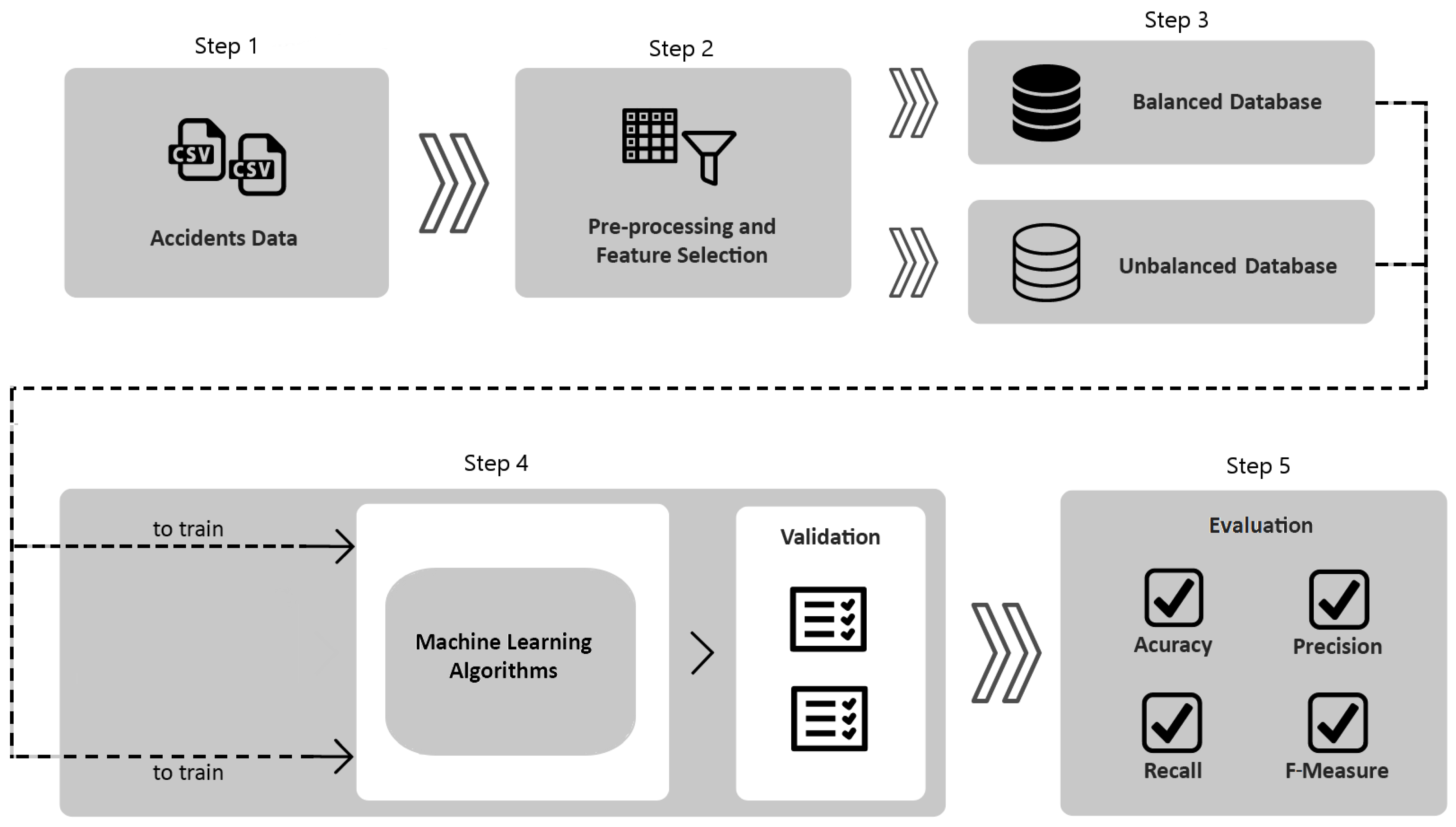
In this work, we propose a five-step method to identify sections of Brazilian highways with a risk of severe accidents. First, we collected data from the Brazilian Federal Highway Police. Some pre-processing techniques are applied to the data, including creating new features. To avoid redundant data, we selected features using LIME as a strategy. The data are naturally imbalanced, so we constructed another version to balance and assist machine learning algorithms to avoid overfitting. We built and trained the machine learning models with the data to evaluate and interpret the results (Figure 4). Each step is detailed in the following sections.

3.1. Data Gathering

The first step comprises accident data collection. In this study, we collected data from 2007 to 2020 from the Brazilian Federal Highway Police’s publicly available dataset (https://www.gov.br/prf/pt-br/acesso-a-informacao/dados-abertos, accessed on 30 January 2023). That dataset describes accidents that occurred on Brazilian highways. This dataset has approximately 1.8 million entries of accidents. Each entry contains 24 attributes: day of occurrence, day of the week, country state, accident location identification (highway, kilometer, county), accident type, a severity rating, the direction of the road, meteorological condition, number of highway lanes, highway layout description, zone (either urban or rural), number of people (involved, dead, minor injuries, severely injured, unharmed, unknown) and the number of involved vehicles.

Table 1. Features from PRF data.

Feature	Description
date	Date of occurrence in format yyyy/mm/dd. E.g., 2017/12/01
weekday	Day of the week of occurrence. E.g., Segunda, Terça, etc.
time	Time of occurrence hh:mm:ss. For example: 08:30:45
uf	Brazilian state of occurrence. E.g., MG, PE, DF, etc.
br	Represents the highway of the occurrence. E.g., 101, 230, 116, etc.
km	Represents the highway kilometer of the occurrence. E.g., 10, 50, 114, etc.
city	City of the occurrence. For example: Campina Grande, São Paulo, Salvador, etc.
accident_cause	Identification of the probable cause of the accident. E.g., lack of attention, incompatible speed, etc.
accident_type	Identification of the type of accident. E.g., head-on collision, lane departure, etc.
accident_classification	Classification according to the severity of the accident: without victims, with injured victims, with fatal victims and ignored.
day_part	Phase of the day at the time of the accident. E.g., dawn, midday, midday and dusk.
road_direction	Direction of the road considering the point of collision. For example: ascending and descending.
weather_condition	Meteorological condition at the time of the accident. E.g., clear sky, rain, sun, hail, wind, cloudy and snow.
road_type	Road type considering the number of tracks. E.g., single, double or multiple.
road_layout	Description of the road layout. E.g., straight, curve, bridge, crossing and tunnel.
accident_site	Description of the characteristics of the accident site. For example: urban or rural.
people	Total people involved in the incident. E.g., 1, 2, etc.
dead_people	Total people dead in the incident. E.g., 0, 2, etc.
minor_injuries	Total people with minor injuries involved in the incident. E.g., 0, 1, etc.
major_injuries	Total people with major injuries involved in the incident. E.g., 1, 2, etc.
total_injuries	Total number of injured people involved in the incident (sum of major and minor injuries). E.g., 1, 2, 3, etc.
unharmed	Total number of unharmed people involved in the incident. E.g., 0, 1, etc.
unknown	Total number of people involved in the incident whose physical status was unknown. E.g., 1, 2, etc.
vehicles	Total number of vehicles involved in the incident. E.g., 1, 2, 3, etc.

depicts the features used.

Because the primary goal of this research is to propose an approach to identify areas with a risk of severe accidents in Brazilian highways, we created a class attribute that we named “severity”. This custom attribute can assume the values “severe” or “nonsevere” according to the number of people with minor injuries, severely injured, and dead from each accident. Thus, these numbers inform the features: dead, minor_injuries, severely_injured and unharmed. We consider an accident severe if there are any victims and severely injured people. In contrast, we consider it nonsevere if there are only minor injuries or unharmed people. So, we also removed the attributed number of people, deaths, minor injuries, severely injured, injured, unharmed, ignored, and accident classification because these attributes are correlated with that class.

This derived attribute indicates whether a highway section is considered severe or nonsevere according to the number of minor and serious injuries and victims of each accident, informed by the numerical dataset attributes: died, serious_injured, light_injured, and unharmed. We developed an algorithm in which an accident is considered severe if it has victims (died > 0) and/or serious injuries (serious_injured > 0); otherwise, the accident is considered nonsevere.

We created another custom attribute that we named “frequency”. According to Ren et al. [28], it is difficult to predict whether a traffic accident will occur, and for this reason, they have created the “risk” attribute to improve the model that classifies the risk of accidents in Beijing. This “risk” attribute represents the frequency of accidents that occurred in the same time window for a given number of days.

Adapting the “risk” attribute for our study, we propose the frequency of an accident, which is the division of the sum of accidents that occurred in a section of a Brazilian highway by the total number of accidents in the dataset (Equation (1)).

$$f=\frac{{\sum }_{}^{}a(r,k)}{n}$$

(1)

where f is the frequency, $a(r,k)$ are the accidents that have occurred on highway r at kilometer k, and n is the total number of registered accidents.

3.2. Pre-Processing and Selection

After collecting the data, the second step is responsible for preprocessing the collected data and selecting relevant features for this study. It was necessary to perform preprocessing on the dataset to remove spelling inconsistencies and simplify similar values. In addition, the vast number of features in the dataset and the complexity of the importance of these features made the classification a complex task. Thus, selecting the most significant features for this study was necessary.

We used numbers for the categorical features and normalized them between 0 and 1 to avoid biases. The original dataset was filled using text so that there were different phrases to describe the same thing. For example, in the column representing the weather (climate) at the time of the accident, we had: a sunny, clear day and full sun to describe the same state: “sunny”. We filtered all cases and simplified these descriptions, normalizing the data. After normalizing the data, we assigned a unique number, ranging from 0 to 1, to each attribute. For example, the “day of the week” has seven possible values. Thus, each day of the week received a unique value representing the day: Monday—0.1, Tuesday—0.2, Wednesday—0.3, and so on.

To identify relevant attributes to this study, we used the LIME (Local Interpretable Model-agnostic Explanations) [29] tool. The LIME tool has a class called Explainer, which uses a classification model to identify the attributes that are relevant or not to classify an instance of a given dataset. In this research, we used Random Forest as the Explainer classifier model for being a classifier that handles imbalanced data well [30].

Initially, we trained the model with accident data according to the “severity” class. Thereby, we used the LIME to explain, for a random instance, the attributes that have most contributed to the classification, among which is the probability of that instance being a true positive. We performed this analysis on many cases. We then conclude that the attributed number of vehicles, land use, date of the accident, and county do not contribute to the data classification. After the feature selection task, the final attributes were the following: the Federation Unit with highway identifier, the kilometer of the highway, day of the week, time of the day, number of lanes, the direction of the route, type of road layout, meteorological condition (good—clear sky/sun/cloudy or stormy—rain/hail/fog/mist), type of accident (collision, rollover or running over), and severity indication.

3.3. Dataset Balancing

After the preprocessing and feature selection step, the third step of our proposed method consists of creating two datasets: a balanced and an imbalanced dataset. There is a significant disproportion between the number of accidents considered to be “severe” (313,176) and those considered to be “nonsevere” (1,537,513). The usage of imbalanced data may compromise the performance of machine learning algorithms [31], so we proposed the construction of a balanced dataset. To accomplish that goal, we used a random undersampling technique, which randomly removes instances of the majority class [31], resulting in 313,176 accidents considered to be “severe” and 314,000 accidents considered to be “nonsevere”. The two versions have the same attributes, and there is no structural difference between the two data.

3.4. Training and Prediction

The fourth step of our method involves applying machine learning algorithms to recognize accidents. We compare three algorithms for this goal: ANN, SVM, and AutoML TPOT.

One of the most popular classifiers is SVM (Support Vector Machine) [24]. Due to its extensive usage and promising results [32], we used the SVM implementation available on the scikit-learn library [33], using different kernels, such as linear, RBF, Sigmoid, and polynomial. We also estimate the C parameter using the GridSearch approach.

Another classifier used was ANN, an artificial neural network. This model can produce good results once it learns an adequate representation of the available features, which can be very useful in the context of accident data features. This model comprises an input layer that receives the preprocessed data directly connected to two fully combined (or dense) sequential hidden layers, each with four nodes. The last layer, the output layer, returns the risk of an accident in a highway section, given the accident. Each hidden layer uses the Rectified Linear Unit (RELU) as the activation function, while the output layer uses the Sigmoid as its activation function. We train the network for five epochs, with batch_size = 64 and learning_rate = 0.1. These parameters were manually calculated for the model.

These algorithms have parameters that must be estimated to guarantee the best performance for the specific problem. Additionally, the algorithm itself could be considered a hyperparameter. We apply an Automl technique called TPOT [34,35] to automate this step. TPOT implements genetic optimization to decide the best classifier and hyperparameters to be used. At each generation, some classifiers and hyperparameters are chosen as individuals to be evaluated.

3.5. Evaluation

All models were evaluated with 10-fold cross-validation. Using the cross-validation technique allows us to partition the dataset into n mutually exclusive subsets, which will use n-1 subsets for training the model and the remaining subset for testing.

Each experiment was measured by Accuracy (Acc), Precision (Pr), Recall (Rc), and F1-score (F1). We assessed these metrics for each performed experiment, and at the end of the study, we identified and pointed out the best techniques and settings for the intended purpose.

4. Experiments and Results

This section describes the setup used to run all the performed experiments. We also present the results of all of these experiments to validate the proposed method, along with a brief discussion of the results.

4.1. Experiment Setup

We used Python and R scripts, executed in a machine with 16 GB of RAM, an Intel Core i7 3.4 GHz CPU, and 1 TB of disk storage, running Windows 10 as the operating system. We also ran the experiments in the same machine using the classification algorithms described in the previous section.

Because they are computationally expensive, we conducted the experiments that use TPOT using Google Colaboratory (https://colab.research.google.com/, accessed on 30 January 2023), Google’s machine learning research and education tool, which provides a virtual code execution machine with 12.6 GB of RAM, 320 GB of disk storage, an Intel Xeon 2.3 GHz CPU with 45 MB of cache and an NVIDIA Tesla K80 graphics card, with 2496 CUDA cores, and a VRAM of 12 GB GDDR5. The database we used for storing the structured data was PostgreSQL (https://www.postgresql.org/, accessed on 30 January 2023). For the execution of the classification algorithms, we used the implementations available in the scikit-learn library Python, using the Jupyter Notebook (https://jupyter.org/, accessed on 30 January 2023).

4.2. Attribute Analysis

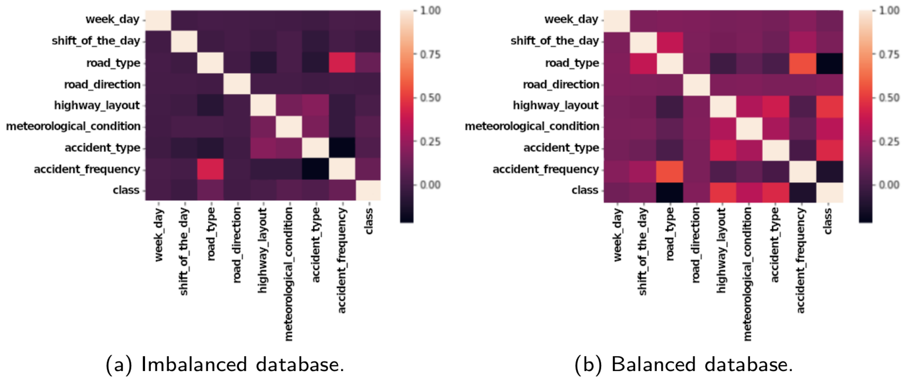
Firstly, we perform attribute analysis to understand both data distribution and correlation. We calculated the correlation between the final features in each dataset to enable the visualization of which attributes could be the most influential when classifying highway sections.

Figure 5a depicts the correlation between the attributes for the imbalanced dataset, while Figure 5b shows the same correlation for the balanced dataset. Comparing both plots, we note that the correlation between the attributes for the imbalanced dataset is low. For the balanced dataset, there is a correlation between the accident class, the highway layout, and the type of accident. The frequency and road type also correlate, as well as the accident type, highway layout, road type, and day shift in which the accident occurred.

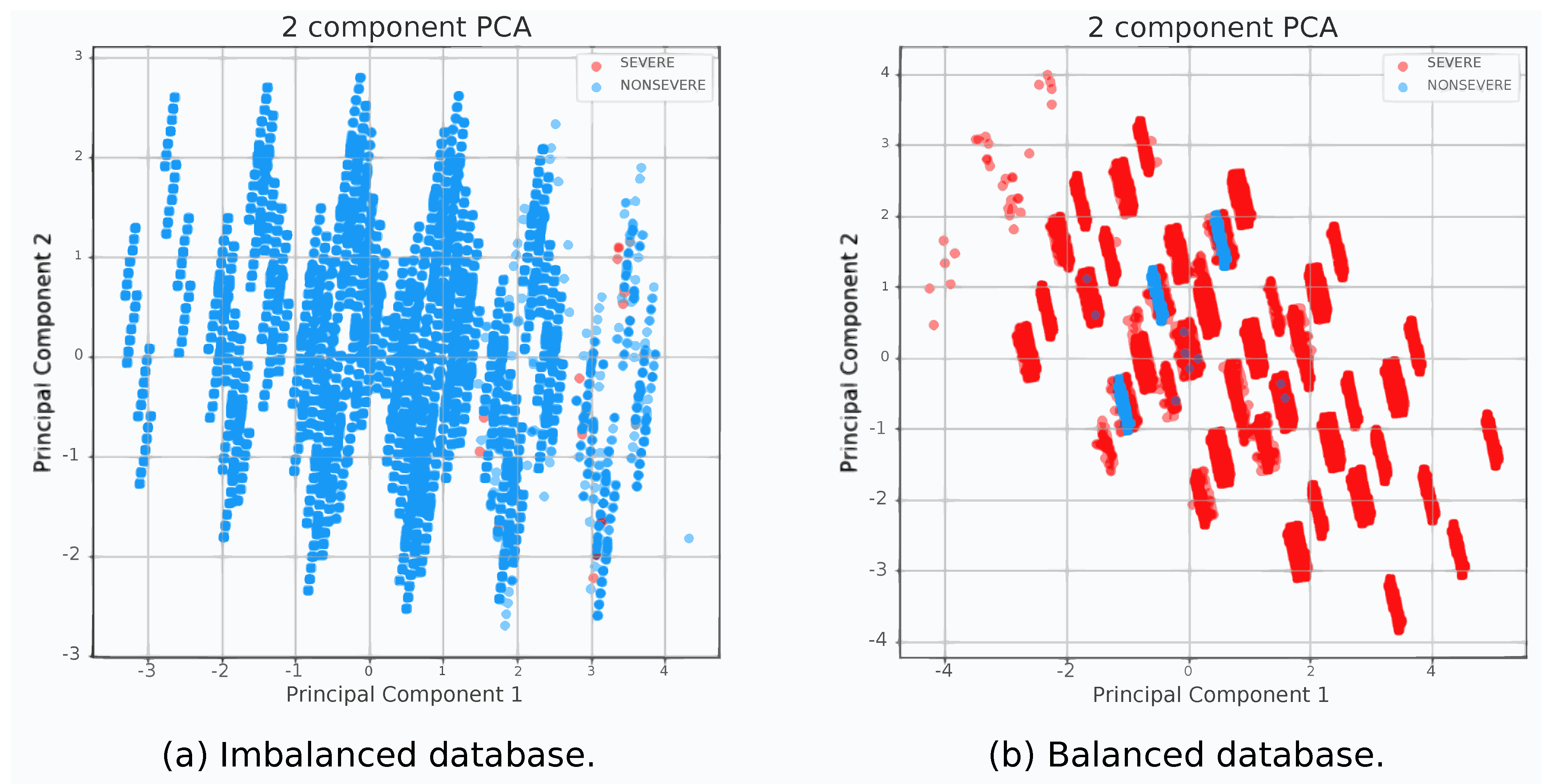
To improve the visualization of possible data patterns, we created two scatter plot visualizations, one for the imbalanced dataset, presented in Figure 6a, and another one for the balanced dataset, detailed in Figure 6b. Hence, the PCA technique was used to represent data in a two-dimensional plane [36].

Figure 6a shows the dispersion of imbalanced data, where the number of instances considered to be “nonsevere” is larger than the number of instances considered to be “severe”. Most instances considered to be “severe” are next to each other in the range 1 to 4 of the X-axis (Principal Component 1) and −1 to 2 of the Y-axis (Principal Component 2).

Figure 6b shows the dispersion of the balanced data. We can note that when reducing the dimensionality and having a balanced dataset, the instances considered to be “nonsevere” were grouped between −2 to 2 of the X-axis (Principal Component 1) and −1 to 2 of the Y-axis (Principal Component 2), while the instances considered to be “severe” became more dispersed. Nevertheless, with the balancing of the dataset, the classes have a much smaller volume of intersections, indicating that there may be a simpler classifier, linear or close to it, capable of distinguishing the classes. Therefore, by balancing the dataset, it was also possible to reduce the complexity of the classification problem.

4.3. Experimental Results

In our experiments, we used a balanced dataset and an imbalanced dataset, which were tested with and without the “frequency” attribute. The balanced dataset has 313,176 accident instances that are considered to be “severe” and 314,000 accident instances that are considered to be “nonsevere”. In comparison, the imbalanced dataset has 313,176 accident instances considered to be “severe” and 1,537,513 accident instances considered to be “nonsevere”. We then evaluated which classifier could better predict the risk of severe accidents on Brazilian highways.

4.3.1. Results using Artificial Neural Network

We conducted two experiments using an artificial neural network. The first experiment did not consider the “frequency” custom attribute for both the balanced and imbalanced datasets. The second study also included the “frequency” custom attribute for both the balanced and imbalanced datasets.

In the first experiment, without the “frequency” attribute and using the imbalanced dataset, the model accuracy reached 82%, while the precision scored 69%, the recall achieved 82% and the F1-score was 75%. However, since there is a significant difference in the number of instances of the “severe” class compared to the “nonsevere”, the model classified most samples in this test as “nonsevere”.

Using the balanced dataset without the “frequency” attribute, the accuracy of the model reached 80.6%. At the same time, the precision, recall, and F1-score also achieved 80.6%. The classifier was able to classify instances in the “severe” and “nonsevere” classes. We note that the problem of the previous experiment (in which the model ignored one of the classes), which used the imbalanced dataset, was solved.

In the second experiment, in which we included the “frequency” attribute and used the imbalanced dataset, our results were: 82% accuracy, 69% precision, 82% recall, and 75% F1-score. Similar to the previous experiment using the imbalanced dataset, in this second experiment, the model also ignored the “severe” class; in other words, it classified all instances as “nonsevere”.

Using the “frequency” attribute and the balanced dataset, we could avoid the problem of classifying all instances into the same class. This new experiment achieved an accuracy of 83%, a precision of 84%, a recall of 83%, and an F1-score of 82%.

Table 2. Results using the artificial neural network, regarding data balancing and the use of the “frequency” attribute.

Balanced	Frequency	Acc	Pr	Rc	F1
No	No	82.00%	69.00%	82.00%	75.00%
Yes	No	80.60%	80.60%	80.60%	80.60%
No	Yes	82.00%	69.00%	82.00%	75.00%
Yes	Yes	83.00%	84.00%	83.00%	82.00%

displays the results of the experiments that used the artificial neural network model. From the experiments, we noticed that using the imbalanced dataset (including or excluding the “frequency” attribute) is not ideal for the goal of this work due to neglecting the “severe” class of an accident. Since we want to know the risk of severe accidents in a highway section, this is the most crucial class in the classification task.

Therefore, considering the performed experiments that used the balanced dataset, it is possible to note that in contrast to the other classifiers, the neural network achieved better results using the “frequency” custom attribute, scoring a superior value in all metrics considered in this study.

4.3.2. Results Using SVM Classifier

Table 3. Results using SVM without “frequency”.

Model	Balanced?	Acc	Pr	Rc	F1
Linear SVM	Yes	58.60%	61.00%	57.90%	59.40%
Linear SVM	No	67.20%	38.80%	67.60%	49.30%
RBF SVM	Yes	57.30%	60.50%	57.40%	58.90%
RBF SVM	No	65.20%	37.00%	65.00%	47.10%
Sigmoid SVM	Yes	56.50%	59.00%	56.20%	57.70%
Sigmoid SVM	No	64.80%	34.10%	64.30%	44.60%
Polynomial SVM	Yes	55.00%	58.20%	54.80%	56.40%
Polynomial SVM	No	64.00%	34.30%	63.50%	44.50%

presents results when using SVM as a classifier and the dataset without the “frequency” custom feature. Among the obtained results using the balanced dataset and different SVM kernels, the model that shows better performance is the Linear SVM with higher scores for the F1-score, recall, precision, and accuracy metrics (58.6% accuracy, 61% precision, 57.9% recall, and 59.4% F1-score). This result was found with C = 10 and with the balanced dataset.

The experiments with the “frequency” custom attribute did not present a significant difference compared to the results above. The results using SVM with the imbalanced dataset were not good because the model ignored the “severe” class and classified all the instances as “nonsevere”, showing overfitting in the majority class.

4.3.3. Results Obtained Using TPOT

Table 4. Results using TPOT, regarding data balancing and the “frequency” attribute.

Classifier	Balanced?	Frequency?	Acc	Pr	Rc	F1
DecisionTree + MultinomialNB	No	No	83.07%	81.23%	50.01%	61.09%
XGBClassifier	Yes	Yes	71.25%	71.62%	71.24%	71.13%
LogisticRegression + RandomForest	No	Yes	70.12%	70.63%	70.11%	69.97%
ExtraTrees	No	Yes	70.07%	70.6%	70.06%	70.06%
DecisionTree + XGBClassifier	Yes	Yes	71.13%	71.75%	71.12%	70.92%
XGBClassifier	Yes	No	83.09%	69.72%	50.11%	55.63%
DecisionTree	Yes	No	83.08%	41.54%	50.00%	45.38%

presents the results obtained using TPOT as a classifier. TPOT was configured with a default package and sparse data. This package contains algorithmic classifier implementations such as DecisionTrees, ExtraTrees, XGBoost, LogisticRegression, and RandomForest. TPOT will estimate both classifier and hyperparameters. Additionally, it could combine several classifiers, making an ensemble.

The XGBClassifier has the best result in terms of F1-score and was chosen as the most adequate for the balanced dataset using the “frequency” attribute. The mean of the results of this experiment for 10-fold cross-validation was the following: 71.25% accuracy, 71.62% precision, 71.24% recall, and 71.13% F1-score. The use of the balanced dataset solved the classification problem of the “severe” instances. However, the usage of the dataset, including the “frequency” attribute, was not very satisfactory because of its low percentage of correct answers.

4.4. Discussion

As we concluded after the analysis of the experiments, the results found using the imbalanced dataset were not suitable for the goal of this work. These experiments obtained good accuracy, but this finding does not mean the results were good because the other metrics (precision, recall, and F1-score) were low.

Therefore, the comparison among the results considered only the experiments that used the balanced dataset, with or without the “frequency” attribute.

Table 5. Summary of the experimental results.

Classifier	Frequency?	Acc	Pr	Rc	F1
Linear SVM	No	58.60%	61.00%	57.90%	59.40%
ExtraTrees	No	70.07%	70.6%	70.06%	45.4%
LogisticRegression + RandomForest	No	70.12%	70.63%	70.11%	69.97%
DecisionTree + XGBClassifier	Yes	71.13%	71.75%	71.12%	70.92%
XGBClassifier	Yes	71.25%	71.62%	71.24%	71.13%
Artificial Neural Network	No	80.60%	80.60%	80.60%	80.60%
Artificial Neural Network	Yes	83.00%	84.00%	83.00%	82.00%

shows the metrics accuracy, precision, recall, and F1-score, which were obtained during the experiments, with details if we considered the “frequency” attribute or not for that particular experiment.

As we can see in the comparison between the results, the ExtraTrees had the worst performance, followed by the performance achieved by the Linear SVM classifier, for which models were trained using the balanced dataset without the “frequency” attribute.

We achieved the best scores for the evaluated metrics using the artificial neural network model and the XGBClassifier. Additionally, it is worth noting that we trained both models using the balanced dataset considering the “frequency” attribute.

On the other hand, our artificial neural network achieved two good results, those with and without the “frequency” attribute. In addition, comparing the experiment performed using the “frequency” attribute improves the metrics. It obtained a growth in the recall of 2.4 pp. and 3.4 pp. for precision and increased the accuracy by 1.4 pp. These higher metric values tell us that this attribute’s usage helped the classifier improve the prediction of the risk of accidents on highway sections. It is also worth noting that the neural network, the XGBClassifier, and the ensemble of DecisionTree + XGBClassifier were the only classifiers that achieved better results when using the “frequency" attribute. All of the other classifiers did not perform well when using this feature.

Comparing the artificial neural network using the “frequency” attribute and the XGBClassifier also using the “frequency” attribute, we observed considerable differences between the metrics of such experiments. The F1-score of the neural network is 10.87 pp. higher. It also improved the precision by 11.76 pp., while the recall grew by 12.38 pp., and the accuracy is 11.75 pp. higher.

Our results surpassed the state-of-the-art, as seen in

Table 6. Comparison of results with the literature.

Work	Algorithms	Acc	F1
Proposed Method	Neural Network	83.00%	82.00%
Tiwari et al. [37]	Lazy Classifier (IBK)	84.47%	-
Kumar et al. [8]	Random Forest	81%	-
Satu et al. [23]	J48 (pruned)	78.9%	-
Iranitalab and Khattak [24]	KNN and K-means	73.95%	-
Tambouratzis et al. [22]	Neural Network and DecisionTree	70%	-
Bülbül et al. [19]	CART	-	81.1%
Tiwari et al. [38]	Decision Tree	-	71.8%
Zhang et al. [39]	K-means and Bayesian network	-	59%
Yu et al. [40]	Neural Network	-	73.65%

. We managed to improve the classification of accident data according to their severity, making viable the usage of the classifier in identifying Brazilian highway sections with a risk of severe accidents.

Our approach reaches excellent results in comparison with the related works. We could highlight the best F1-Score, even in a cross-validation experiment. Only Tiwari et al.’s [38] work had greater accuracy than our approach. However, the authors did not provide precision, recall, and f1-score to make a fairer comparison.

5. Conclusions

Most recently, the scientific community has proposed methodologies for identifying segments or sections of roads and highways with a risk of accidents. The motivation of this field of study is to discover solutions that help to decrease the number of accidents. The accidents’ location is an essential feature due to its singularities.

This work aimed to classify, using several features, sections of Brazilian federal highways according to their risk of accidents, which can be severe or nonsevere. A highway section considered to be severe indicates that, given a set of features, that section is prone to the occurrence of severe accidents.

The results showed that some supervised machine learning techniques produce good classifications depending on the given attributes and dataset. Our tests using the imbalanced data did not present good results. Our source code and dataset are available at the URL below, to enable the reproducibility of our experiments: (https://github.com/lsi-ufcg/risk-of-accidents, accessed on 30 January 2023).

In the experiments using the balanced dataset with the “frequency” attribute, the neural network model provided the best results, achieving an accuracy of 83%, a precision of 84%, a recall of 83%, and an F1-score of 82%.

For future work, we will develop a smartphone app that uses the studied classification algorithms to alert the driver of the potential risk of a severe accident in certain highway sections. The app would warn the driver of areas on his route with the risk of severe accidents. The app would also consider external variables collected in real-time (such as the day of the week, time of the day, weather conditions, etc.). These data would be the input for the classifier, which would then return the sections with the possibility of severe accidents. We would also use nonofficial sources of accident data to increase our dataset—for example, we could use the information gathered by Twitter and Waze.