SLBRIN: A Spatial Learned Index Based on BRIN

Abstract

The spatial learned index constructs a spatial index by learning the spatial distribution, which performs a lower cost of storage and query than the spatial indices. The current update strategies of spatial learned indices can only solve limited updates at the cost of query performance. We propose a novel spatial learned index structure based on a Block Range Index (SLBRIN for short). Its core idea is to cooperate history range and current range to satisfy a fast spatial query and efficient index update simultaneously. SLBRIN deconstructs the update transaction into three parallel operations and optimizes them based on the temporal proximity of spatial distribution. SLBRIN also provides the spatial query strategy with the spatial learned index and spatial location code, including point query, range query and kNN query. Experiments on synthetic and real datasets demonstrate that SLBRIN clearly outperforms traditional spatial indices and state-of-the-art spatial learned indices in the cost of storage and query. Moreover, in the simulated real-time update scenario, SLBRIN has the faster and more stable query performance while satisfying efficient updates.

1. Introduction

In the current normal environment of COVID-19, location-based services (LBS) have become an important part of the infrastructure of people’s daily lives [1]. It produces real-time spatial big data, and meanwhile, exposes the urgency of spatial interoperability. For instance, we record our trips (data update) and query the epidemic distribution (spatial query) frequently through various terminal devices. In database management systems (DBMS), indexing is a powerful means to speed up a query by trading space for time. There are also plenty of spatial indices for spatial data [2], of which the most typical is R-tree [3]. However, with the increasing complexity of spatial big data, the bottlenecks of traditional spatial indices are emerging [4], such as a large cost on storage and queries.

Learned indices [5], a new direction for DBMS, simplify the index relationship between the index value and the physical location into a nonlinear regression function. Henceforth, more and more studies have introduced learned indices into geographic information science (GIS), eventually forming the spatial learned index. Spatial learned indices mainly solve four problems: (1) Order spatial data: due to spatial heterogeneity [6], it is difficult to quantify the spatial proximity through a single dimension. Most spatial learned indices just map spatial data into one-dimensional values by dimensionality reduction, i.e., via a space-filling curve (SFC) [7,8], i-Distance [9]. (2) Homogenize distribution: homogenizing the data distribution makes its cumulative distribution function (CDF) easier to learn, thereby improving the training efficiency and query performance, such as quantile transformation [10] and rank space ordering [11]. (3) Partition data: the partitioned index, with a higher overall accuracy, are mainly divided into two types, i.e., data-based partition and spatial-based partition [12]. (4) Handle update: the update strategies of spatial learned indices basically follow that of the normal learned index.

Existing spatial learned indices, benefiting from learned indices, have lower cost of storage and query. However, the methods to fit spatial data also complicate the index structure. In addition, their update strategies sacrifice a certain amount of query performance and only support a limited number of updates. Block range index (BRIN) [13] and BRIN-Spatial [14] divides index entries into ranges along the physical order and statistics summary info as index values, naturally taking the smallest size and the fastest update. When data are stored in order, their monotonic summary info offers the best query performance. Index update should not only guarantee the update performance, but also reduce the query performance penalty. However, current spatial indices are caught in the conflict between them, such as R-tree and Learned Index structure for Spatial dAta (LISA) [15] (weak in update), and BRIN-Spatial (weak in query).

With the purpose of optimizing both query performance and update performance, we propose a novel spatial learned index structure, SLBRIN. Its core idea is to simplify the problem of spatial index by dividing the index object into two parts: the history range (HR) suitable for spatial query and the current range (CR) suitable for index update, and optimize the processing strategies with the spatio-temporal features of spatial big data. For HR, the spatial fields are first encoded and sorted to form index entries based on Geohash. Then the index entries are partitioned into ranges, with the minimum decimal geohash code as summary info. These ranges are a set of regular quad-partitions with approximate data volume in spatial. Finally, for each range, we build a one-dimensional learned index for spatial queries. For CR, to minimize the update cost, the ranges are partitioned directly along the physical order and take a simple MBR as summary info.

The rest of the paper is organized as follows: Section 2 discusses the related work. Section 3 presents the methodology of our index, including its structure and the strategies in build processing, update processing and query processing. Section 4 provides an extensive experimental evaluation of the proposed work and Section 5 discusses the experimental results. Finally, Section 6 concludes the paper.

2. Related Work

2.1. Spatial Indices

Spatial indices [12] organize spatial data to provide efficient query processing. On the basis of organization, they can be classified into dimensionality reduction, space-based partitioning and data-based partitioning.

Dimensionality reduction maps multidimensional data to one-dimensional values, and then uses one-dimensional indices to index the mapped values. Space fill curves (SFCs) [16] are the most popular, which connect spatial partitions with fractal curves. SFCs mainly include Z-curve [17] and Hilbert-curve [18], as well as their variants, to fit non-point objects [19] and spatio-temporal data [20]. Geohash [21] encodes space with Z-curve and provides advanced methods such as neighbor query. S2 [22] is a method library for three-dimensional space with more refined partitions and shorter codes.

Space-based partitioning divides space recursively based on specific rules and records the mapping relationship between partitions and data. The simplest is grid file [23], which divides space into grids of the same size and uses a hash function to encode grids. KD-tree [24] selects dimensions iteratively and build a binary search tree for multidimensional data. Quadtree [25] and octree [26] use four and eight nodes to achieve uniform partition in two and three dimensions, respectively. Point range quadtree [27], a variant of quadtree, controls the volume of leaf nodes to make partitions closer to the data distribution.

Data-based partitioning relies on the data distribution, with strong query performance, but also high update cost. The most classic is R-tree [3], a B-tree with MBR as summary info. Each node of R-tree stores a set of MBRs and the pointers to child nodes or index entries. There are lots of variants of R-tree, such as STR-tree [28] to accelerate index construction and R⁺-tree [29] and R^*-tree [30] to solve spatial overlap. Additionally, Q⁺R-tree [31] and Hilbert R-tree [32] mix other indices to improve performance, and TPR-tree [33] adapts to spatio-temporal data. Unlike R-tree, BRIN [13] is not based on the spatial distribution, but the storage order. BRIN divides pages into ranges along the physical order with an extremely low update cost. BRIN is designed for handling very large tables in which certain columns have some natural correlation with their physical location. BRIN-Spatial [14] extends BRIN by using MBR as summary info. Its query processor only searches the index entries within certain ranges of which the MBR intersects with the query.

2.2. Learned Indices

Learned indices interpret indices as a function that take the query condition as input and physical location of data as output. They take a regression model instead of the traditional indices to solve this function. Kraska et al. [5] proposed the learned index, as well as recursive-model indices (RMI) for the last-mile search of big data. From then on, the studies on the learned index mainly focus on index update and dimension expansion.

Index update. In response to any updates, the learned index must retrain models to ensure the validity of error bounds, which is costly in time. ASLM [34] partitions data with the maximum intervals, and uses cache as a transfer for updates. Hybrid-LR [35] stores outliers separately in B-tree to stabilize model accuracy. FITing-tree [36] reserves extra physical space for each partition. IFB-tree [37] evaluates the update cost with interpolation-friendliness, such as a partition in uniform distribution with higher interpolation-friendliness. PGM-index [38] admits a streaming algorithm to partition, instead of using FITing-tree’s greedy algorithm, and handles updates using LSM-tree. Shift-table [39] resolves the local biases of learned models at the cost of (at most) one memory lookup.

Dimension expansion. The index is built for query requirements. Spatial learned index is a special learned index, taking coordinates as queries. To learn spatial distribution, the first challenge is to order spatial data. SageDB [40] sorts data based on the specified dimension and learns the granularity of partitions automatically based on data distribution and query distribution. Similar to KD-tree, Flood [41] sorts and partitions multidimensional data based on each dimension. ZM-index [7], HM-index [8], ML-index [9] and LISA [15] use Z-curve, Hilbert-curve, i-Distance, and Lebesgue Measure respectively to reduce dimensionality. Some studies replace deep learning models with piecewise linear functions [36] and spline interpolation functions [42] to improve model accuracy. Similarly, PolyFit [43] and SPRIG [44] fit spatial distribution using piecewise polynomial functions and spatial interpolation functions to avoid ordering spatial data.

3. Methodology

Our proposed method consists of the overall architecture and the strategies in building, updating and query processing.

Table 1. Notation.

Notation	Definitions
P	a spatial dataset
d, n, S	dimensionality, cardinality and scope of P
L	length of Geohash
HR, CR	history range and current range
M	a learned model
IE	an index entry
TN, TL	thresholds for HR’s number of IEs and actual geohash length
TS	threshold for CR’s number of IEs
TM	threshold for the number of CRs
TE	threshold for M’s error bounds

lists some important notations.

3.1. SLBRIN Architecture

The core concept of BRIN is range (Definition 1). The summary info of range is the key to judge whether the target exists in range. The most commonly used summary info is the minimum and maximum of all index entries in those pages. The ranges may overlap, and the degree of overlap determines their query performance. To process queries, BRIN collects the eligible candidate pages by simply scanning all the summary info. BRIN-Spatial, the spatial variant of BRIN, takes MBR as its summary info, as shown in

Table 2. The summary information of BRIN,BRIN-Spatial and SLBRIN.

Range ID	Pages	BRIN (Min, Max)	BRIN-Spatial/SLBRIN CR (xmin, ymin, xmax, ymax)	SLBRIN HR (gmin)
0	1, 128	0, 8	0, 0, 4, 4	0
1	129, 256	2, 7	1, 1, 8, 8	4
2	257, 384	4, 9	2, 0, 7, 2	8

.

Definition 1.

A range is a group of the fixed disk page units (128 pages per range by default) and it stores the brief summary information for all index entries in those pages as a query filter.

Our SLBRIN goes beyond BRIN and extends the range to HR and CR. For HR, we first used Geohash to order spatial data. Geohash uses base-32 to reduce the code length and accelerate the prefix match, but raises the likelihood of jumping nature. Therefore, we retreated to base-10 to have a more reasonable spatial representation. IEs are sorted by the decimal geohash code both among and within HRs, and thus HRs are strictly non-overlapping in spatial. We can only use their minimum IEs’ key as the summary info, as their maximum is equal to the minimum of the next HR. As the summary info is monotonic (ordered and unique), we designed the decimal geohash match (DGM) based on a binary search to find out the candidate HR. Given that the prefix match of Geohash can only use ‘=’, DGM takes full advantage of the monotonicity to use ‘>’ and ‘<’ additionally. As in Algorithm 1, A is the summary info of all HRs and q is the decimal geohash of query point. If A_mid = q, then HR_mid contains q. If it is not found in the end, then HR_right contains q.

Algorithm 1: Decimal Geohash Match

Input: A: a sorted decimal geohash array; q: a geohash query; (l, r): the initial left and right. Output: the key to q. 1: while l ≤ r do 2:   mid$\leftarrow$(l + r)/2 3:   if Amid = q then 4:     return $mid$ 5:   else if Amid < q then 6:     l$\leftarrow$mid+1 7:   else 8:     r$\leftarrow$mid-1 9: return r

For CR, new IEs in a specific time period are temporarily stored in CRs. The front CR is merged into HR first and stores the oldest IEs. The temporal proximity of spatial distribution indicates the continuity of CRs in time, which means CRs are likely to overlap in spatial. So, unlike HR, we simply used the MBR as its summary info.

As shown in

Table 3. SLBRIN objects.

Physical Object	Logical Object	Attributes
Meta Page	Meta	int32 *lastHR, int32 *lastCR, int8 L, 5 × int16 thresholds
HR Pages	HR	int64 value, int8 len, int16 num, int32 *model, int8 state
CR Pages	CR	4 × int64 value, int16 num, int8 state
Model Pages	M	Matrix matrices, int32 minErr, int32 maxErr
Data Pages	IE	int64 geohash, d × float64 spatialFields, int32 *data

, SLBRIN’s structure is mainly composed of five physical objects and five logical objects.

(1) Meta Page records the metadata, including the pointers of the last HR and the last CR, the length of the geohash L and five thresholds of TH, TL, TS, TM and TE. The two pointers help to locate the most active range quickly when handling updates; TH and TL determine the spatial granularity of HR, which is related to query performance; TS, TM and TE are used to trigger the three parallel operations in update processing.

(2) HR Pages record HR in pages with attributes as follows: (a) value records the minimum decimal geohash code as summary info; (b) len and num record the actual geohash length and current volume of IEs to assist in partitioning HR; (c) *model records the pointer of M in Model Pages; (d) state records whether HR is inefficient.

(3) CR Pages record CR in pages. CR is simpler than HR, only containing three attributes: (a) value records the MBR as summary info; (b) num records the current number of IEs; (c) state records whether CR is full or outdated.

(4) Model Pages record all Ms in pages. The attribute matrices records the slope and bias of each layer and minErr and maxErr define the error bounds. The approximate physical location of the target can be calculated directly by matrix operations, and the exact physical location can be found by a second scan within the error bounds.

(5) Data Pages record all the IEs in pages. IEs take the decimal geohash code as the key and the physical location as the value, and preserve the spatial fields to assist queries. In the logical structure, both HR and CR store IEs. However, in the physical structure, Data Pages store all the IEs, while HR Pages and CR Pages only store the metadata of ranges.

3.2. Build Processing

We present the details of SLBRIN through its build processing as Algorithm 2. (1) For spatial data as Figure 1a, we reduced its dimensionality and sorted it by Geohash to build ordered IEs as Figure 1b. (2) We recursively partitioned HR with IEs and built the physical structure of SLBRIN as Figure 1c. Since there is no update in build processing, CR is empty. (3) For each HR, we built the learned model by learning its spatial distribution, which is the main way to filter IEs within HR.

3.2.1. Ordering Data

(1) Calculate geohash length. Geohash partitions space in the way of recursive dichotomy. The deeper the recursive level R of Geohash, the smaller the unit scope of partitions. Equation (1) shows that once the unit scope is more refined than the data precision, Geohash encodes all the data uniquely. Based on this, the minimum recursive level R_min can be derived as Equation (2), where S_i is the scope in the i-th dimension, S_R is the unit scope in level R and prec is the data precision.

Algorithm 2: Build SLBRIN

Input: P: a spatial dataset; (TH, TL, TS, TM, TE): the thresholds Output: I: our index. 1: calculate the geohash encoding length of P to L 2: calculate and sort IEs by Geohash(L) to ieList 3: initial rangeStackand rangeList 4: rangeStack.push(CreateRange(0, 0, P.size, [0, P.size - 1])) 5: while rangeStack.size ≠ 0 do 6:   range$\leftarrow$rangeStack.pop(-1) 7:   if range.num > TN and range.len < TL then 8:     initial childs; lk, rk$\leftarrow$range.keyBound; tlklk 9:     for i$\in$[0, 3] do 10:         len$\leftarrow$range.len + 2; value$\leftarrow$range.value + (i << L - len) 11:         breakpoint$\leftarrow$range.value + (i + 1 << L - len) 12:         trkDGM(ieList, breakpoint, tlk, rk); num$\leftarrow$trk – rlk + 1 13:         childs.push(CreateRange(value, len, num, [tlk, trk])); tlk$\leftarrow$trk + 1 14:     rangeStack.push(Reverse(childs)) 15:   else 16:     rangeList.push(range) 17: create HR for each range in rangeList and store to HR Pages 18: create empty CR and store to CR Pages 19: create Meta and store to Meta Page 20: reorganize ieList and store to Data Pages 21: build and train M and store extract args to Model Pages 22: return I

$$S_R=\underset{\forall i\in d}{\min }\left\{S_{i,max}-S_{i,min}\right\}/2^R\le prec$$

(1)

$$R_{min}=\lfloor {\log }_2\left(\underset{\forall i\in d}{\min }\left\{S_{i,max}-S_{i,min}\right\}/prec\right)\rfloor$$

(2)

(2) Encode single dimension. Geohash dichotomizes coordinates recursively in each dimension and records the binary value for each dichotomy. Since R_min is determined, the geohash code can be calculated directly with simple bit operations as in Equation (3), where v_i is the coordinate in the i-th dimension and bin(x) means to obtain the binary of x. If the geohash length is less than R_min, it must be completed with 0 on the left side.

$$g_i=\mathrm{bin}(\frac{v_i-S_{i,min}}{S_{i,max}-S_{i,min}}\times (1\ll R_{min}\left)\right)$$

(3)

(3) Merge geohash codes. The geohash codes in each dimension were cross-merged into single code of length L = d $\times$ R_min. We further compressed geohash codes to the decimal to reduce the cost in storage and query.

(4) Build IE. IE is more compact than data itself in physical space, which can reduce the IO cost of spatial query. We took the decimal geohash code as the key of IE and then sorted all the IEs by their keys.

3.2.2. Building SLBRIN

The build processing of SLBRIN was carried out around HR, which was similar to point range quadtree [27] in terms of partitioning.

(1) Initial range. The beginning of recursion is the initial range for all IEs. We recorded the start pointer and end pointer of IEs in keyBound for each range. All the ranges to be partitioned were recorded in a stack rangeStack, of which the first member was the initial range. In addition, the eligible ranges were recorded in a linked list rangeList (Lines 3–4).

(2) Partition recursively. Partitioning of HR results in a set of ranges that satisfy the condition num < TN and len < TL (Lines 5–16). TN balances the volume of IEs among HRs. However, the aggregation of spatial data is likely to bring about a deep partition, especially an infinite partition when its scope is refined than its precision. To avoid this, we used TL to limit the actual geohash length. The details of partitioning are as follows: (a) Iterate over each range in rangeStack; (b) If the range does not meet the condition, find the quartiles of keyBound by DGM, partition into four children and push into rangeStack; (c) Else, push into rangeList. The children are a quarter of their parent in spatial, so their len and value (l and v in short) can be derived from their parent using Equations (4) and (5).

$$l_{child}=l_{parent}+2$$

(4)

$$v_{child,i}=v_{parent}+\left(i\ll L-l_{child}\right), 0\le i<2^d$$

(5)

(3) Create SLBRIN. We created the logical and physical objects. For HR, we transformed each range in rangeList to HR and store them into HR Pages. For CR, empty CRs are enough for build processing, as there is no update. For Meta, we extracted the pointers of last HR and CR, as well as the thresholds and L, and stored them into Meta Page.

(4) Reorganize IEs. The physical space of range is of the same size and continuous. However, the IEs mapped by keyBound are in varying quantities, so we reorganized and stored them into Data Pages. When num ≥ TN and len ≥ TL, the physical space cannot store all the IEs of the HR. To solve the overflow of IEs, we created empty pages at the end of HR Pages and recorded the pointer of these pages as an external link in the HR.

3.2.3. Building Learned Model

(1) Build model. Dimensionality reduction transforms the independent variable of index from multi-dimensional spatial fields to one-dimensional geohash code. After ordering, data are unordered in physical location. Instead, we took the ordered physical location of IE as the dependent variable and constructed a learnable CDF, as in Equation (6).

$$p.key=F\left(p.cord\right)\times n\underset{}{\Rightarrow }F\left(Geohash\left(p.cord\right)\right)\times n$$

(6)

The physical location of IE in Data Pages is only continuous within HRs, so we used piecewise nonlinear function to fit its CDF. A piecewise nonlinear function can be described as Equation (7), where M_i is the unary nonlinear relation of the i-th HR, and $\beta =\left({\beta }_0,{\beta }_1,···,{\beta }_{\sigma }\right)$ is a set of breakpoints.

$$F\left(x\right)=\{\begin{array}{c}{M}_0\left(x\right), {\beta }_0\le x<{\beta }_1\\ M_1\left(x\right), {\beta }_1\le x<{\beta }_2\\ \dots \dots \\ M_{\sigma }\left(x\right), {\beta }_{\sigma }\le x<{\beta }_{\sigma +1}\end{array}$$

(7)

To solve F, we only needed to solve $M_i$, as breakpoints are known as the adjacent values. We ensured that the monotonicity was not only within but also among HRs to achieve the overall monotonicity of F. As in Equation (8), each $M_i$ is monotonic and the left border should not be smaller than the right border of the previous.

$$M_i\uparrow \cap M_i\left( {\beta }_i\right)\ge M_{i-1}\left( {\beta }_i\right)$$

(8)

Following the first learned index [5], we chose multi-layer perceptron (MLP) to learn the non-linear function rather than the other regression model. We built an MLP with one hidden layer and sigmoid activation function, as in the universal approximation theorem: An MLP, with a linear output layer and at least one hidden layer with enough neurons and any kind of squeezed activation function, can fit any Borel measurable function from one finite dimensional space to another with any accuracy [45].

(2) Define error bounds. For the multi-staged spatial learned indices, such as the RMI version of ZM-index [7] and RSMI [11], the upper stage tends to take larger error bounds than the lower, or worse, resulting in the overall unsatisfactory error bounds. SLBRIN takes a hash function (DGM) as the upper stage, and thus its error bounds exist within HRs, which guarantees the last-mile search and reduces the overall error bounds.

The error extremes are as important as the overall fitting degree, which is directly related to the query performance. As in Equation (11), we used a weighted sum of cross entropy and error extremes as the loss function, explaining the fitting degree and error extremes respectively, where $w$ is the weight to eliminate the impact of different units.

$$e{g}_{min}=\underset{\forall x\in P}{\min }\left\{M\left(x\right)-y\right\}$$

(9)

$$e{g}_{max}=\underset{\forall x\in P}{\max }\left\{M\left(x\right)-y\right\}$$

(10)

$${ℒ}_M=\frac{1}{n}{{\displaystyle \sum }}_{\forall x\in P}{\left(M\left(x\right)-y\right)}^2+w\times \left(e{g}_{max}-e{g}_{min}\right)$$

(11)

(3) Train and extract model. For M_i, the training data are all the IEs of HR_i, as well as the breakpoints value_i and value_i+1 for the constraint in Equation (8). We normalized the training data by the maximum and minimum, choose Adam as the optimizer and used the early stopping mechanism to shorten the training time. After training, to reduce the cost of storage and query, we extracted the weights and error bounds from the complex deep learning framework, and stored them into Model Pages.

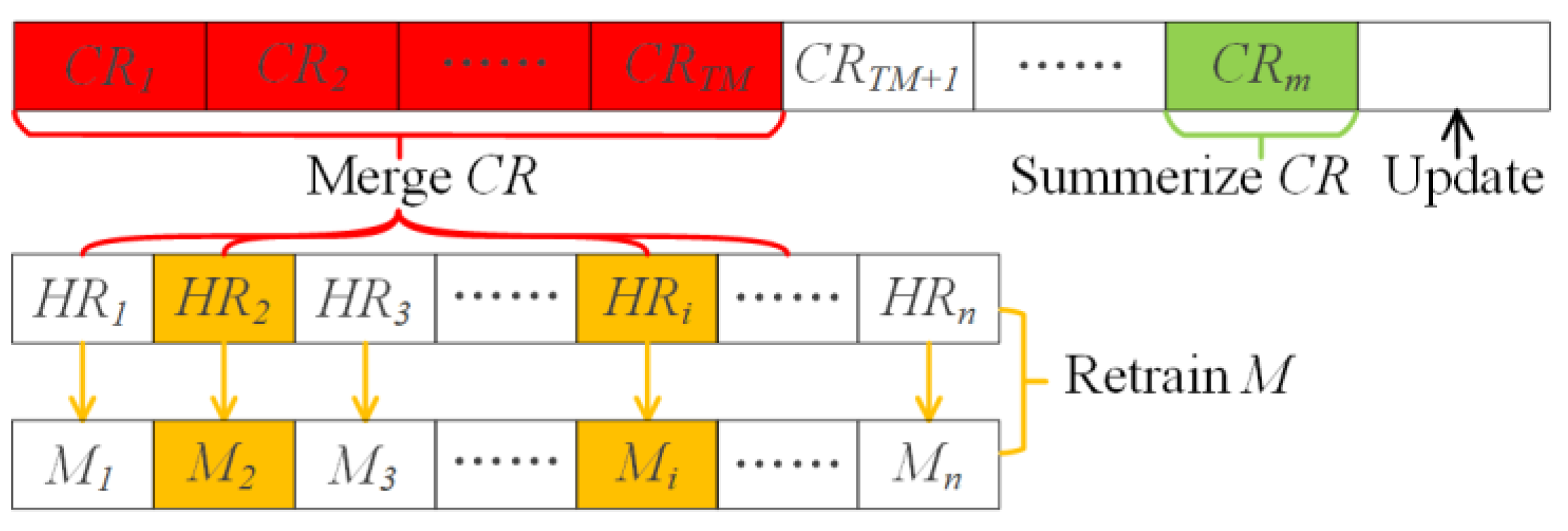
3.3. Update Processing

Algorithm 3 shows the pseudo code of the update handling in SLBRIN. The cascading operations of data update are deconstructed into serial operations and parallel operations. Serial operations are blocking to keep the data consistency, i.e., the next update cannot be started until the current serial operation is completed. Parallel operations are non-blocking and triggered by pre-defined conditions, including summarize CR, merge CR and retrain model, as shown in Figure 2. We further divided them into two sub-operations, GET and POST, to improve parallelism.

Algorithm 3: Update SLBRIN

Input: p: the data item to be updated; I: our index. 1: g$\leftarrow$Encode(p, I.meta.L) 2: ie$\leftarrow$(g, p.spatialFields, p.key) 3: lastCR $\leftarrow$I.meta.lastCR 4: lastCR.num$\leftarrow$lastCR.num + 1 5: I.data.append(ie) 6: Listening Trigger: 7:   lastCR.num > TS$\Rightarrow$ summarize full CRs 8:   (lastCR – lastHR)/size(CR) > TM$\Rightarrow$ merge outdated CRs 9:   newErr/oldErr > TE$\Rightarrow$ retrain models of inefficient HRs

(1) Build IE. As with build processing, we first encoded the updated data by Geohash and built the new IE (Lines 1–2). To simplify the modification and deletion of data, we unified them as insertions. For example, the modification takes the modified value as key, while deletion takes null as key.

(2) Insert to CR. The new IE is stored in CR temporarily and will be persisted into HR after merging CR. The specific operation is to increment the attribute num of the last CR, and append the new IE to Data Pages (Lines 3–5).

(3) Summarize CR (Parallel). Summarizing CR aims to create summary info to enhance the performance of the last CR. In most cases, only the last CR needs to be summarized, but given that it takes time to summarize, multiple CRs may be summarized at the same time. If queries come when the last CR is not full, the summarizing can be advanced passively. (a) GET: monitor the num of the last CR; once num reaches TS, update the attribute state to 1 and append an empty CR to the last CR Pages. (b) POST: collect all the full CRs (state = 1); for each full CR, summarize MBR, update value with MBR and reset status.

(4) Merge CR (Parallel). Merging CR aims to transfer IEs from CR to HR to decrease the slow query in CRs and increase the fast query in HRs. We merged only the oldest TM CRs to decouple from the IE insertion. (a) GET: monitor the total number of CRs; once the number reaches TM, update the state of the first TM CRs to 2. The number of CRs can be calculated based on the attributes *lastCR and *lastHR of Meta using Equation (12), where size(CR) is the physical size of CR. (b) POST: collect all outdated CRs (state = 2); partition all the IEs of the outdated CRs into several parts by the way of HR partitioning (Lines 5–19 of Algorithm 2); match all the IE parts and HRs on the same geohash code, and merge their IEs in Data Pages; delete the first TM CRs from CR Pages.

$$n_{CR}=\frac{*lastCR-*lastHR}{size\left(CR\right)}$$

(12)

(5) Retrain M (Parallel). After merging CR, we needed to correct the error bounds for models relative with the updated HRs. The retraining model aims to reduce the error bounds for all updated models to stabilize their query performance. (a) GET: monitor the attributes minErr and maxErr of the updated models; once the new error bound exceeds the old error bound by TE times, update the state of its relative HR to 1. (b) POST: collect all inefficient HRs (state = 1); for each inefficient HR, retrain its model with the new IEs, update it into Model Pages and reset state. Before retraining, we also used breakpoints to maintain the monotonicity in Equation (8).

The temporal proximity of spatial distribution shows that spatial data in continuous time have similar spatial distribution [46]. In other words, given a spatio-temporal dataset with the spatial distribution as D, when its cardinality is sufficient, its sub-dataset at any time has the similar spatial distribution to D. Based on this, we propose the following two hypotheses for SLBRIN:

• For overall HR or any CR, in case of sufficient IEs, the spatial distribution tends to D.
• The scope of the local range can be encoded uniquely as g by Geohash. For any local range, in case of sufficient IEs, its spatial distribution D_g tends to the part of D in the scope g.

In real-time spatial scenarios, the IEs in HR and CR are often sufficient to support these hypotheses. Even for the insufficient IEs, the insignificant trends in the hypotheses are still beneficial for optimizing the update processing.

Based on hypothesis 1, the overall HR has the optimal query performance as its spatial distribution tends to D. However, the opposite is true for CR. When the spatial distribution of CR tends to D, the spatial filtering ability of MBR degrades rapidly. So, TS should be small enough to avoid hypothesis 1 to hold in CR.

Based on hypothesis 2, for any range during merging CR and any HR, its spatial distribution only depends on its geohash code. Therefore, we used DGM to solve the Cartesian product between the outdated CRs and HRs, reducing the time complexity of merging CR from O(nm) to O(n + m), where n and m is the number of ranges. From another perspective of hypothesis 2, the ranges with the same scope have similar spatial distribution. After merging CR, for the updated HRs, their old models have a certain ability to fit the new spatial distribution. So, we only updated their error bounds based on Equations (9) and (10) rather than retraining.

The updated HR may be partitioned into several child ranges, whose models can inherit from the parent HR without retraining. In d = 2, we took the first of the four child ranges as an example to present the derivation process of model inheritance:

• The child’s input domain [−0.5, 0.5] corresponds that of parent [−0.5, −0.25], so the input layer of MLP is calculated as follow:

$$Y=Sigmoid\left(W_i\left(0.25\left(Y^T+0.5\right)-0.5\right)+B_i\right)$$

(13)

2.

The child’s output domain [0, 1] corresponds that of parent [M(−0.5), M(−0.25)], so the output layer of MLP is calculated as follow:

$$Y=\frac{\left(W_o{Y}^T+B_o\right)-M\left(-0.5\right)}{M\left(-0.25\right)-M\left(-0.5\right)}$$

(14)

Above, M(x) is the attribute matrices of parent model, W_i, B_i, W_o, and B_o are the slope and bias of M(x) of the input and output layers, respectively. In summary, the model inheritance of the first child is as shown in Equations (15) and (16).

$$W_i=0.25W_i,B_i=-0.375W_i+B_i$$

(15)

$$W_o=\frac{W_o}{M\left(-0.25\right)-M\left(-0.5\right)},B_o=\frac{B_o-M\left(-0.5\right)}{M\left(-0.25\right)-M\left(-0.5\right)}$$

(16)

Inefficient HR means that its learned model no longer tends to D_g, which is basically caused by three cases: (1) The old IEs are not sufficient resulting in that the old distribution does not reach D_g. (2) The new IEs are not sufficient resulting in that the overall distribution is deviated from D_g. (3) The long-term accumulated error bound eventually reaches TE. In either case, the old learned model can still fit D_g to some extent, and thus we can initialize the new model with the attribute matrices of old model to shorten the retraining time and narrow the error bound.

3.4. Query Processing

Based on the SLBRIN’s structure, we designed the query strategy based on learned index and spatial location code, including point query, range query and kNN query. We also considered the repetition of spatial data during the query processing.

3.4.1. Point Queries

Given a query point p, the target keys may exist in both HRs and CRs. The query processing, as shown in Algorithm 4, can be detailed into the following three steps:

Algorithm 4: Point Query

Input: p: a point query; I: our index. Output: result: the key to p. 1: crLsit$\leftarrow$search cr from I.CRs where cr.value ⸧ p 2: result$\leftarrow$search ie from crLsit where ie = p 3: g$\leftarrow$Encode(p, I.Meta.L) 4: hr$\leftarrow$DGM(I.HRs, g) 5: model$\leftarrow$hr.model 6: pre$\leftarrow$model.predict(g) 7: result.push(MBS(I.IEs, pre, model)) 8: return result

(1) Filter CRs. The MBR and IEs of CR are both unordered. To collect the target keys in CRs, we traversed all the CRs to find the candidate CRs whose MBR contains p, and then filter the IEs in all candidate CRs (Lines 1–2).

(2) Filter HRs. The value of HR is monotonic decimal geohash code. To compare with it, we encoded p to g and then use DGM to find the candidate HR (Lines 3–4).

(3) Filter in HR. The IEs in candidate HR can be filtered by replicating the forward propagation of MLP (Lines 5–6). It mainly includes three steps: (a) Normalize g with the values of candidate HR and its next HR as the minimum and maximum. (b) Compute the result by matrix operations with g, as in Equation (17), where the output of each layer is used as the input of the next layer, and the last layer does not use activation function. (c) Inversely normalize the result with the physical space of HR, and finally obtain the predicted physical location pre of the query point p.

$$Y=Sigmoid\left(W{Y}^T+B\right)$$

(17)

As the principle of learned index [5], p.key must lie within the error bound, as in Equation (18), which can be found out by Model Biased Search (MBS) (Line 7). The difference of MBS from binary search is that its initial position is pre, which is more suitable for the learned index.

$$p.key\in \left[pre-e{g}_{max},pre-e{g}_{min}\right]$$

(18)

3.4.2. Range Queries

Range query aims to find all the targets falling in the query range qr. Similar to point query, it also requires the filtering of both CRs and HRs, as shown in Algorithm 5.

Algorithm 5: Range Query

Input: qr: a range query; I: our index. Output: result: the keys falling in qr. 1: crList$\leftarrow$search cr from I.CRs where cr.value ∩ qr 2: result$\leftarrow$search ie from crList where ie ⸦ qr 3: pb, ptqr; gb, gt$\leftarrow$Encode([pb, pt], I.Meta.L) 4: rangeList$\leftarrow$GeohashRangeQuery(gb, gt) 5: range.hr$\leftarrow$DGM(I.HRs, range.g) for each range in rangeList 6: group rangeList by range.hr and merge range.pos 7: for each range in rangeList do 8:   get gb, gt with range.pos; preb, pret$\leftarrow$range.hr.model.predict([gb, gt]) 9:   keyb, keyt$\leftarrow$MBS(I.IEs, [preb, pret], range.hr.model) 10:   for k$\in$[keyb, keyt] do 11:     if iek ⸦ qr then 12:       result.push(k) 13: return result 14: 15: function GeohashRangeQuery(gb, gt) 16:   initial rangeList; l$\leftarrow$Max(Len(gb), Len(gt)) 17:   gxb, gyb, gxt gyt$\leftarrow$Decode([gb, gt], l) 18:   gxl$\leftarrow$gxt - gxb; gyl$\leftarrow$gyt - gyb 19:   gList$\leftarrow$Encode(gx, gy, L) for gx$\in$[gxb, gxt], gy$\in$[gyb, gyt] 20:   for g in gList do 21:     pos$\leftarrow$ check position by gxl, gyl 22:     rangeList.push(CreateRange(g, pos)) 23:   sort rangeList by range.g 24:   return rangeList

(1) Filter CRs. We filtered CRs to find the candidates whose MBR intersects qr, and then filtered the candidates to obtain the target keys contained by qr (Lines 1–2).

(2) Filter HRs. Figure 3 shows the process to filter HRs, where the grid layout represents the spatial distribution of HRs. In line 3, qr is simplified to the decimal geohash codes g_b and g_t of the bottom-left corner p_b and top-right corner p_t, as shown in Figure 3a. The judgement of whether qr contains p is also simplified as Equation (19).

$$\underset{\forall i\in d}{p.cor{d}_i}\in \left[q{r}_{i,min},q{r}_{i,max}\right]\stackrel{}{\Rightarrow }{g}_p\in \left[g_b,g_t\right]$$

(19)

For ordered data, we can obtain the key range only by the left and right bounds of qr. However, Geohash is not a complete order, so qr contains several key ranges of geohash code in most cases. We designed the geohash range query method to find the candidate HRs and determine their spatial relationship with qr. As shown in Algorithm 5, we used a separate function GeohashRangeQuery() to show its details.

• Calculate the granularity of candidate ranges. A moderate granularity helps to filter HRs effectively. The granularity l lies between the maximum geohash length of all candidate ranges and L. We used the larger geohash length of g_b and g_t, which yields the best performance in experiments (Line 16).
• Decode g_b and g_t into one-dimensional geohash code gx_b, gy_b, gx_t, gy_t by Geohash, and calculate the number of candidate ranges along horizontal and vertical directions as gxl and gyl (Lines 17–18).
• Create the Cartesian product by all one-dimensional geohash codes in the domain of [gx_b, gx_t] and [gy_b, gy_t], and encode each member by Geohash as gList (Line 19).
• In spatial, each range in gList is contained or intersected by qr. In lines 20–22, we marked the spatial relationship between range and qr with the spatial location code, which consists of four binary bits, indicating that range intersects the bottom, top, left, right of qr, respectively. For example, a spatial location code of [1 0 0 0] means the range intersects the bottom of qr. Based on the order of the Cartesian product, we confirmed that the first gxl ranges intersect the bottom of qr, and the last gxl ranges intersect the top of qr. In addition, the ranges whose sequence is divisible by gyl intersect the left of qr, and their previous ranges intersect the right of qr. All the others are contained by qr, initialized as [0 0 0 0]. As a range has multiple spatial relationships with qr, the spatial position codes can be combined with the OR operation, i.e., [1 0 0 0] | [0 0 1 0] = [1 0 1 0] means the range intersects the bottom and left corner of qr, and [1 1 1 1] means the range contains qr.
• Sort rangeList by decimal geohash code (Line 23).

As shown in Figure 3b, the candidate ranges in rangeList are a set of grids with uniform spatial scope, and are inconsistent with HRs in terms of geohash length. So, we need to solve the many-to-many connections between candidate ranges and HRs, which can be accelerated by DGM. As shown in Figure 3c, we finally obtained all the candidate HRs as well as their spatial location codes (Lines 5–6).

(3) Filter in HR. First, we obtained the two corners g_b and g_t of the spatial intersection between HR and qr with spatial location code. Then, we used a learned model to obtain the predicted physical locations key_b and key_t and form a key range of [key_b, key_t] (Lines 8–9). Due to the jumping nature of SFC, the IEs within the key range were probably not contained by qr. So, a second scan was required. We simplified the judgement in Equation (19) using spatial position code. For example, we only judged p.cord_y ≥ bottom for the HR intersecting the bottom of qr, and there was no second scan for the HR contained by qr.

3.4.3. kNN Queries

We designed a bottom-up kNN query strategy as Algorithm 6. As CR is not friendly to kNN query, we filtered HRs first to narrow the query scope for CR. Given a point p and a number k, we used a priority queue pQueue to store the target keys. It always contained k points with the smallest distance to p. The query processing is as follows:

(1) Filter HRs. We found the key key_p of p by point query (Algorithm 4). Then, we selected k points nearby key_p as the initial result and offer their distance to p into pQueue (Lines 2–5). The current maximum distance of initial result is dst. The jumping nature of SFC is likely to bring about a larger dst. However, its probability can be reduced by selecting redundant points. We selected k points before and after key_p as the initial result, a total of 2k + 1 points, which offer the best performance in experiments. The selection process may cross HRs because of the discontinuity of the physical locations. To solve this, we jumped the pointer with the help of the logical object of HR.

Algorithm 6: kNN Query

Input: p: a point of kNN; k: a positive number of kNN. Output: pQueue: a priority queue contains the nearest k keys to p. 1: pQueue$\leftarrow$PriorityQueue((-1, +∞), k) 2: keyp$\leftarrow$PointQuery(p) 3: for key $\in$[keyp - k, keyp + k] do 4:   pQueue.offer(key, Distance(p, pkey)) 5: dst$\leftarrow$pQueue.peek() 6: construct qr with p and dst 7: pb, pt$\leftarrow$qr; gb, gt$\leftarrow$Encode([pb, pt], I.Meta.L) 8: rangeList$\leftarrow$GeohashRangeQuery(gb, gt) 9: range.hr$\leftarrow$DGM(I.HRs, range.g) for each range in rangeList 10: group rangeList by range.hr and merge range.pos 11: range.dst$\leftarrow$Distance(range.hr, p) for each range in rangeList 12: sort rangeList by range.dst 13: for each range in rangeList do 14:   if range.dst > dst then 15:     break 16:   else 17:     get gb, gt with range.pos; preb, pret$\leftarrow$range.hr.model.predict([gb, gt]) 18:     keyb, keyt$\leftarrow$MBS(I.IEs, [preb, pret], range.hr.model) 19:     for k$\in$[keyb, keyt] do 20:       pQueue.offer(key, Distance(p, pkey)) 21:     dst$\leftarrow$pQueue.peek() 22: update qr by dst 23: crList$\leftarrow$search cr from I.CRs where cr.value ∩ q 24: pQueue.offer(keyie, Distance(p, ie)) for each ie in crList 25: return pQueue

It is known that the maximum distance to p of the targets must be smaller than dst. To find the candidate HRs, we created a query range qr with p as center and dst as radius, and performed a range query with qr (Lines 6–11). In contrast to range query, we sorted the candidate HRs by their distance to p in positive order (Line 12).

(2) Filter in HR. For each candidate HR, we offered all the IEs to pQueue and updated dst at the end of each loop (Line 13–21). Once the distance of candidate HR exceeds dst, we broke the loop early, as all the subsequent candidates were out of the query scope.

(3) Filter CRs. For the range query of CR, the smaller the query range, the greater the filtering ability of MBR. After filtering in HR, the query scope of pQueue is close enough to the scope of targets, which is efficient to filter CRs. We took the latest dst of pQueue as the radius of qr, and performed a range query with qr for CR (Lines 22–24). Eventually, all the points in pQueue are the targets of kNN query.

4. Experiments

In this section, we report on the experimental studies that compare SLBRIN with selected alternative methods.

4.1. Experimental Settings

All experiments were implemented in Python 3.7.10 and executed on a 64-bits Ubuntu 16.04 with a 3.50 GHz Intel Xeon CPU E5, 8 GB RAM and a 1 TB hard disk.

Datasets. We used the following spatial datasets. Each dataset is sorted by the temporal field. We selected the first half to build indices and test the query performance, and inserted the other half into indices to test the update performance.

• NYCT is a historical repository of 750 million rides of taxi medallions over a period of four years (2010–2013) in New York City [47]. We extracted the part of January and February 2013, about 28,236,977 records (2.84 GB in size), with the pickup time as temporal field and the pickup coordinates as spatial fields.
• UNIFORM and NORMAL are synthetic datasets in uniform and normal distributions. The synthetic data falls into the unit square, with a random temporal field and the same cardinality as NYCT (1.58 GB in size).

Competitors. We compared with the following indices:

3.

R-tree [3] (RT): The most typical spatial index.

4.

Point range quadtree [27] (PRQT): A variant of quad-tree, balancing the cardinality between partitions with a threshold, similar to HR.

5.

BRIN-Spatial [14] (BRINS): The spatial variant of BRIN with MBR as summary info.

6.

Z-order model [7] (ZM): A classical spatial learned index using Z-curve to reduce dimensionality. We used Geohash instead of Z-curve for ease of comparison.

7.

LISA [15]: A spatial learned index structure designed for disk-resident spatial data, which has shown strong query performance.

Implementation. We used the original implementation of all the competitors following their papers. The environment variables were set as follows: page size was 4096 bytes, address size was 4 bytes and the spatial fields and decimal geohash code were stored in double (8 bytes) and long integer (8 bytes), respectively. For RT, we used a node capacity of 113 and stored a single node per page. For PRQT, we implemented the breadth-first search version with a threshold of 500, which shows the best performance during grid search. For BRINS, we sorted data by Geohash and took 64 pages per range. For SLBRIN, ZM and LISA, we used the same MLP and determined the hyper-parameters as learning_rate = 0.1, batch_num = 64, w = 10.

Evaluation Metrics. To evaluate the performance of all competitors, we used three kinds of metrics. For build processing, we used index size to show storage cost and build time to show build performance. For query processing, we used query time and IO cost to show query performance. Query time indicates the average response time for a query; IO cost indicates the average number of pages to be loaded for a query, which serves as an important indicator for the index based on external memory. For update processing, we used update time to show update performance, which indicates the average response time of for an update.

4.2. Effect of Thresholds

We first study the effect of the five thresholds on the performance of SLBRIN.

TL. TL is the maximum level of HR partitioning, which ensures HR’s spatial scope is always larger than the data precision. Generally, TL is less than L, which is calculated by the scope and precision of dataset (Section 3.2). We set TL = 40, when L = 52 for all datasets.

TN. TN is the maximum number of HR’s IEs. If HR stores more IEs than TN during the building processing or update processing, it needs to be partitioned. In addition, TN is closely related to the query performance of HR, so we built SLBRIN on NYCT with TN varying from 5 K to 20 K and report the range query performance. As shown in Figure 4a, increasing TN always increases the IO cost. This is expected because the larger TN brings about the larger error bounds, resulting in filtering out more unqualified IEs. However, the average query time decreases and then increases progressively. That is because when TN is less than 10 K, the cost to filter HRs is more expensive than the cost to filter the IEs within HRs. So, we set TN = 10 K which has the lowest query time.

TS. Corresponding to TN, TS is the maximum number of CR’s IEs and is related to the query performance of CR. We also varied TS from 5 K to 20 K and insert NYCT into an empty SLBRIN, so as to only test the range query performance of CR. As shown in Figure 4b, the average query time presents a down and up trend, whereas the lowest value turns out at TS = 10 K, as the best TS is a trade-off between filter CRs and filter IEs. According to hypothesis 1 (Section 5), the spatial distribution of large CR tends to S, which lowers the earning of filtering CRs. In other words, although the number of CRs decreases, the number of candidate CRs increases, and more IEs need to be filtered. We set TS = 10 K.

TM. TM is the number of CRs to be merged into HRs at one time. Since HR outperforms CR in query performance, we should handle as many CRs as possible in update processing. In a production environment, we adjust TM dynamically according to the actual update workload. We set TM = 50 for ease of experiments.

TE. TE is the critical ratio of error bound to trigger the model retraining for HRs. After merging CRs, we update the error bounds for all relative HRs. However, HRs are retrained only when their error bounds are TE times the old. The smaller the TE, the more frequent the retraining, but also the better the query performance of HR. We recommend setting TE = 1.5 to reduce the frequency of model retraining properly.

4.3. Build Performance

The first set of experiments studies the build performance under different datasets.

Index size. The index size contains two parts: (1) IE size. BRINS, ZM, LISA and SLBRIN, are all larger than the others (387.4 MB vs. 276.7 MB), as they record the mapped geohash code additionally. (2) Index structure size, as shown in Figure 5a. R-tree (660.4 MB) is the largest, even larger than its IEs because it stores a large number of MBRs. It is followed by PRQT (5.9 MB) that stores only a small amount of MBRs. BRINS (0.04 MB) is the smallest, indicating that the storage cost of range is extremely low. Under the premise of the same number of sub-models, SLBRIN is smaller than ZM and LISA, which also benefits from range structure (7.2 MB vs. 7.4 MB, 18.6 MB).

Build time. Figure 5b reports the build time across data distribution. RT and PRQT are 1394.3 s and 238.8 s, respectively. BRINS (115.3 s) is the fastest because both writing IEs sequentially and summarizing range have low IO cost, which is the same with CR of SLBRIN. Due to training models, HR of SLBRIN, ZM and LISA are the slowest (2636.9 s vs. 2752.0 s, 8797.3 s), which can be accelerated with GPU and multi-process. With RTX 1080 Ti GPU and 5 parallel processes, SLBRIN reduces the build time by 8.2 times (320.0 s), but ZM only reduces by 5.9 times (469.5 s) and LISA only reduces by 4.3 times (1795.4 s). This is because the concurrency of ZM and LISA is limited within stages and the lower stage will wait for the upper stage to calculate the training data. In contrast, SLBRIN, directly partitioned based on data distribution, offers higher concurrency in build processing.

4.4. Point Query Performance

The second set of experiments studies the point query performance under different datasets. We randomly sampled 1000 points in each dataset as query points, and report the query time and IO cost per point query.

Query time. Figure 6a reports the query time across different datasets. SLBRIN offers the best query performance on both synthetic and real datasets. It improves the query time by at least 2.8 times and up to 6.3 times compared with the competitors, i.e., 41.5 µs vs. 117.3 µs (ZM) and 260.0 µs (LISA) on NYCT. In the order of UNIFORM, NORMAL and NYCT, the complexity of spatial distribution and the query time for all competitors both increase. For example, RT and PRQT are 69.3 µs and 125.0 µs on UNIFORM, but increase to 258.4 µs and 154.0 µs on NYCT. This is because, under the complex spatial distribution, PRQT and the spatial meaning of RT tend to be unbalanced indicating the performance degradation. In contrast, BRINS, ZM and LISA are more stable, 150.0 µs, 115.1 µs and 265.3 µs for all datasets, indicating the query performance of range and learned index are more stable in terms of spatial distribution. Inheriting both advantages, SLBRIN holds lower error bounds, the shortest query time (41.2 µs), and the strongest stability.

IO cost. Figure 6b reports the IO cost across different datasets, and SLBRIN also improves by at least 1.3 times and up to 3.7 times. On NYCT, BRINS is the highest (308.6), as it needs to filter all IEs within a specific range. RT and PRQT spend 9.0 and 12.7 on filtering the tree structure and a specific leaf node. SLBRIN has a lower IO cost than ZM and LISA (7.8 vs. 38.5 and 8.0). This is because SLBRIN optimizes the spatial partition of range and uses the spatial learned index to lower the IO cost within range.

4.5. Range Query Performance

The third set of experiments studies the range query performance under different data distributions and different query range sizes. We generated 1000 random windows within the scope of each dataset as query ranges and report the query time and IO cost per range query.

Varying the data distribution. As Figure 7a,b shows, SLBRIN offers the best query performance on all datasets and the largest improvement on NYCT across all datasets. On NYCT, compared with the competitors, it improves the query time by at least 9.8 times and up to 76.4 times (0.2 ms vs. LISA’s 2.3 ms and ZM’s 17.9 ms), and improves the IO cost by at least 1.7 times and up to 30.1 times (67.1 vs. LISA’s 115.9 and ZM’s 2018.6). Conversely, ZM and LISA show the worst performance on NYCT than the other datasets. In addition, ZM shows the worst performance of all competitors, as the jumping nature of SFC makes its range queries filter out vast invalid IEs. It indicates that SLBRIN learns the spatial distribution better, and its range query strategy with spatial location code effectively reduce the filtering of IEs.

Varying the query range size. We varied the query range size from 0.0006% to 0.16% of the dataset scope and report the query time and IO cost on NYCT as Figure 7c,d. The query performance of SLBRIN is optimal for all range sizes, and the larger the range size, the higher the improvement. We measured the stability of query performance over range size by the growth ratio of query time. When the range size is small, RT takes on a natural advantage in filtering nodes and has a query performance close to SLBRIN. When the range size is large, the inefficient filtering of IEs indicates a rapid performance degradation, with a high growth ratio of 2.2. ZM, LISA and BRINS benefit from learned index and range, but also suffer from the jumping nature of SFC. Overall, they have larger query time at all range sizes, but lower growth ratios of 0.2, 1.0 and 0.8. SLBRIN offers a low growth ratio of 0.7, indicating its query performance is more stable across query range size.

4.6. kNN Query Performance

The fourth set of experiments studies the kNN query performance under different data distributions and different ks. We randomly generated 1000 kNN queries within the scope of each dataset and report the query time and IO cost per kNN query. BRINS and ZM do not come with a kNN algorithm, so we used RSMI’s kNN algorithm [11] for them.

Varying the data distribution.Figure 8a,b reports the kNN query performance across different datasets. BRINS and ZM offer the highest query time (14.3 ms and 18.8 ms) and the largest IO cost (369.1 and 691.2). In contrast, SLBRIN yields the best query performance and the strongest stability across data distribution, with a stable query time of 0.29 ms and a low IO cost of 10. This indicates SLBRIN’s kNN query strategy effectively reduce the filtering of invalid IEs caused by the jumping nature of SFC. The query performance of RT and PRQT is lower than all the others except SLBRIN, as SLBRIN not only uses the partition of spatial indices, but also has lower error bounds than the other spatial learned indices.

Varying k. We varied the query parameter k from 4 to 64 and report the query time and IO cost on NYCT as Figure 8c,d. Overall, SLBRIN has the best query performance on all ks. In terms of the stability of query time, SLBRIN (0.30) is second only to RT (0.07) in terms of the stability. In terms of the stability of IO cost, SLBRIN (0.10) is third only to PRQT (0.02) and BRINS (0.05). This is expected because ks are much smaller than the capacity of leaf nodes or ranges. ZM and LISA have the worst stability in both terms, i.e., 0.66 and 0.36 in query time, 0.54 and 0.45 in IO cost, indicating SLBRIN takes advantage of the learned index better in the kNN query strategy.

4.7. Update Performance

The fifth set of experiments studies the update performance. We divided the second half of each dataset into five group and inserted each group into the index according to the temporal field. We report the update time and query performance for each group updated points. We also used RSMI’s update algorithm [11] for ZM, as it does not handle updates.

Varying the data distribution. Figure 9a reports the update time across different datasets. BRINS benefits from range and has the lowest update time on all datasets. SLBRIN is faster than ZM and LISA, i.e., 1270.9 s vs. 1925.6 s and 2847.6 s on NYCT. This is because, in addition to the benefit of range, the update strategy based on the temporal proximity of spatial distribution reduces the duration and frequency to retrain the model. However, all the spatial learned indices are slower than RT and PRQT. As with build processing, SLBRIN can also be accelerated by GPU and multi-process, and yields a closer update time to RT and PRQT, i.e., 145.2 s vs. 286.2 s and 149.1 on NYCT.

Varying the updated points. Figure 9b–d report the update time and query performance across the ratio of update points to datasets. BRINS has the lowest update time, but also the highest and fastest rising query time and IO cost, as updated points disrupt its original storage order. With more updates, all competitors increase query time and IO cost, as there are more data to query. For all query scenarios, SLBRIN offers not only the best query performance, but also the strongest stability across index updates. For example, the growth ratios of query time are 0.85 and lower than the best RT of 0.89, and the growth ratios of IO cost are 0.31 and lower than the best LISA of 0.38.

SLBRIN variants. To demonstrate the contribution of each parallel operation to the update strategy, we extended SLBRIN to four variants, as shown in

Table 4. SLBRIN Variants.

Variant	Summarize CR	Merge CR	Retrain M	Retrain M with Old Weights
SBRIN_SCR	√	×	×	×
SBRIN_MCR	√	√	×	×
SBRIN_RM	√	√	√	×
SBRIN	√	√	×	√

. SLBRIN_SCR just summarizes CR. SLBRIN_MCR summarizes and merges CR. SLBRIN_RM retrains models with random weights, which is different from SLBRIN.

We performed the same update experiments for SLBRIN variants on NYCT and report the update time in Figure 10b. We report the error bounds in Figure 10a, which are critical for the performance of the learned index. SLBRIN-SCR’s error bounds are constant and lower than ZM and LISA (268.1 vs. 1400.6 and 466.8), as it does not retrain, and its data-based partition makes HR learn the spatial distribution better. With more updates, the increasing error bounds of SLBRIN_MCR indicate the old models gradually fail to fit the updated distribution. SLBRIN_RM has lower error bounds and a smaller growth ratio than SLBRIN_MCR (340.8 vs. 427.3, 0.54 vs. 1.19), indicating the retraining corrects old models to refit the updated distribution. SLBRIN has the lowest error bounds and the smallest growth ratio (291.3, 0.18), and takes a lower update time than SLBRIN_RM, 1270.9 s vs. 2190.4 s. It indicates that compared with a random initial model, the old model helps the retraining to learn the updated distribution better and faster. In other words, the temporal proximity of spatial distribution contributes to our update strategy. Figure 10c,d report the range query performance. SLBRIN offers the lowest query time (0.8 ms) and IO cost (80.9) across index updates. SLBRIN_SCR has the lowest error bounds, but also has the highest query time of 1.9 ms and IO cost of 95.2, as CR is far inferior to HR in spatial queries.

5. Discussion

In the first experiment, we showed the impact of five thresholds on SLBRIN. (1) TL was calculated by the scope and precision of the dataset. (2) TN and TS are critical to the query performance of HR and CR, respectively. The experiments gave an example to find the optimal value according to the average query time, and we automatically determined TN and TS by means of sample range query in a production environment. (3) Both TM and TE are a trade-off between query performance and update performance. We dynamically adjusted them based on the ratio of queries and updates. For example, when queries are much more than updates, we set TM = max and TE = 1.0 so that merging CR and retraining HR was as frequent as possible to improve the overall query performance.

In the third to fifth experiments, we compared the query performance of SLBRIN with the traditional spatial indices (RT) and state-of-the-art spatial learned indices (LISA). As SLBRIN has the characteristics of range, SFC and spatial partition, we also compared it with BRINS, ZM and PRQT. The experimental results showed that SLBRIN not only offers the best query performance on point query, range query and kNN query, but also has the strongest stability in terms of data distribution, query range size, and k. The reasons are as follows: (1) the index structure based on range is designed for physical storage, which has lower IO cost; (2) the partition of HR is beneficial to fit the spatial distribution and earns lower error bounds; (3) the query strategy with spatial location code effectively reduce the filtering of invalid IEs caused by the jumping nature of SFC.

In the second and sixth experiments, we compared the build performance and update performance of SLBRIN with competitors. Benefiting from learned index and lightweight range, SLBRIN offers lower storage cost and better performance in build processing and update processing. Moreover, SLBRIN exhibits stronger stability of query performance during updates, which is important for real-time spatial scenarios. We extended SLBRIN to four variants and their experimental gaps indicate the effects of three parallel operations and temporal proximity of spatial distribution. Retraining models makes spatial learned indices slower than spatial indices in build processing and update processing, which can be accelerated by GPU and multi-process. For example, the accelerated SLBRIN has the highest optimization ratio and is even faster than RT and PRQT, which indicates SLBRIN has more reasonable spatial partition and more dynamic index structure.

SLBRIN relies on the spatio-temporal continuity of spatial distribution and is not suitable for the irregular or fast-changing scenarios. Although all experiments are based on two-dimensional datasets, all the strategies in SLBRIN, such as HR and spatial location code, are also applicable for multi-dimensional datasets. In addition, both HR and CR can support spatial queries and index updates independently, but yield significant performance shortcomings, which prompts the combination in order complement each other.

6. Conclusions

In this paper, we proposed a novel Spatial Learned index structure based on Block Range INdex, SLBRIN, with the concept of range, history range (HR) and current range (CR). We also provided the update strategy and query strategy to meet the urgent demands of index updates and spatial queries for real-time spatial data. The contributions of this study are summarized as follows:

• For update processing, we deconstructed update transactions into serial and parallel operations to improve parallelism, and made full use of the temporal proximity of spatial distribution to stabilize query performance and improve update performance.
• For query processing, we designed the strategies of point query, range query and kNN query based on the spatial learned index, and optimized them with the spatial partition of HR and the proposed spatial location code.
• Using synthetic and real data, our extensive experiments showed that SLBRIN outperformed all competitors in storage cost, query performance and update performance. Furthermore, SLBRIN offered the strongest performance stability in update processing.

This paper opens up several directions for future research on spatial learned index. First, it is meaningful to adjust the granularity of the spatial location code dynamically based on the workloads. Second, it works in theory to design a more efficient strategy for the spatial join query with spatial location code. Last but not least, the temporal proximity of spatial distribution is capable of giving rise to the spatio-temporal learned index.

References

1. Zhu, Q.; Hu, H.; Xu, C.; Xu, J.; Lee, W. Geo-social group queries with minimum acquaintance constraints. VLDB J. 2017, 26, 709–727. [Google Scholar] [CrossRef]
2. Manolopoulos, Y.; Nanopoulos, A.; Papadopoulos, A.N.; Theodoridis, Y. R-Trees Have Grown Everywhere. Technical Report. 2003, p. 3. Available online: http://www.rtreeportal.org (accessed on 6 January 2022).
3. Guttman, A. R-trees: A dynamic index structure for spatial searching. In Proceedings of the 1984 ACM SIGMOD International Conference on Management of Data, Boston, MA, USA, 18–21 June 1984; pp. 47–57. [Google Scholar]
4. Rigaux, P.; Scholl, M.; Voisard, A. Spatial Databases: With Application to GIS; Morgan Kaufmann: Burlington, MA, USA, 2003; Volume 32, p. 111. [Google Scholar]
5. Kraska, T.; Beutel, A.; Chi, E.H.; Dean, J.; Polyzotis, N. The case for learned index structures. In Proceedings of the 2018 International Conference on Management of Data, Houston, TX, USA, 10–15 June 2018; pp. 489–504. [Google Scholar]
6. Anselin, L. Lagrange multiplier test diagnostics for spatial dependence and spatial heterogeneity. Geogr. Anal. 1988, 20, 1–17. [Google Scholar] [CrossRef]
7. Wang, H.; Fu, X.; Xu, J.; Lu, H. Learned index for spatial queries. In Proceedings of the 20th IEEE International Conference on Mobile Data Management, Hongkong, China, 10–13 June 2019; pp. 569–574. [Google Scholar]
8. Wang, N.; Xu, J. Spatial queries based on learned index. In Proceedings of the 1st International Conference on Spatial Data and Intelligence, Hongkong, China, 18–19 December 2020; Springer: Hongkong, China, 2020; pp. 245–257. [Google Scholar]
9. Davitkova, A.; Milchevski, E.; Michel, S. The ML-index: A multidimensional, learned index for point, range, and nearest-neighbor queries. In Proceedings of the 2020 23rd International Conference on Extending Database Technology, Copenhagen, Denmark, 30 March–2 April 2020; pp. 407–410. [Google Scholar]
10. Hu, L. Efficient Learning Spatial-Temporal Query and Computing Framework for Geographic Flow Data. Ph.D. Thesis, Zhejiang University, Zhejiang, China, 2021. [Google Scholar]
11. Qi, J.; Liu, G.; Jensen, C.S.; Kulik, L. Effectively learning spatial indices. Proc. VLDB Endow. 2020, 13, 2341–2354. [Google Scholar] [CrossRef]
12. Gaede, V.; Günther, O. Multidimensional access methods. ACM Comput. Surv. 1998, 30, 170–231. [Google Scholar] [CrossRef]
13. Herrera, A. Block Range Index. Available online: https://www.postgresql.org/docs/9.6/brin.html (accessed on 6 January 2022).
14. Yu, J.; Sarwat, M. Indexing the pickup and drop-off locations of NYC taxi trips in PostgreSQL—Lessons from the road. In Proceedings of the 15th International Symposium on Spatial and Temporal Databases, Washington, DC, USA, 21–23 August 2017; pp. 145–162. [Google Scholar]
15. Li, P.; Lu, H.; Zheng, Q.; Yang, L.; Pan, G. LISA: A learned index structure for spatial data. In Proceedings of the 2000 ACM SIGMOD International Conference on Management of Data, Dallas, TX, USA, 15–18 May 2000; pp. 2119–2133. [Google Scholar]
16. Sagan, H. Space-Filling Curves; Springer Science & Business Media: New York, NY, USA, 2012; p. 291. [Google Scholar]
17. Ramsak, F.; Markl, V.; Fenk, R.; Zirkel, M.; Elhardt, K.; Bayer, R. Integrating the UB-tree into a database system kernel. In Proceedings of the 26th International Conference on Very Large Data Bases, San Francisco, CA, USA, 10–14 September 2000; pp. 263–272. [Google Scholar]
18. Faloutsos, C.; Roseman, S. Fractals for secondary key retrieval. In Proceedings of the 8th ACM SIGACT-SIGMOD-SIGART Symposium on Principles of Database Systems, Philadelphia, PA, USA, 29–31 March 1989; pp. 247–252. [Google Scholar]
19. Hughes, J.N.; Annex, A.; Eichelberger, C.N.; Fox, A.; Hulbert, A.; Ronquest, M. Geomesa: A distributed architecture for spatio-temporal fusion. In Proceedings of the Geospatial Informatics, Fusion, and Motion Video Analytics V, Baltimore, MD, USA, 20–24 April 2015; pp. 128–140. [Google Scholar]
20. Li, R.; He, H.; Wang, R.; Huang, Y.; Liu, J.; Ruan, S.; He, T.; Bao, J.; Zheng, Y. Just: JD urban spatio-temporal data engine. In Proceedings of the IEEE 36th International Conference on Data Engineering, Dallas, TX, USA, 20–24 April 2020; pp. 1558–1569. [Google Scholar]
21. Ni, E. Geohash. Available online: http://geohash.org (accessed on 6 January 2022).
22. Google. S2 Geometry. Available online: http://s2geometry.io (accessed on 6 January 2022).
23. Nievergelt, J.; Hinterberger, H.; Sevcik, K.C. The grid file: An adaptable, symmetric multi-key file structure. In Proceedings of the 3rd Conference of the European Cooperation in Informatics, Munich, Germany, 20–22 October 1981; pp. 236–251. [Google Scholar]
24. Bentley, J.L. Multidimensional binary search trees used for associative searching. Commun. ACM 1975, 18, 509–517. [Google Scholar] [CrossRef]
25. Finkel, R.A.; Bentley, J.L. Quad trees a data structure for retrieval on composite keys. Acta Inform. 1974, 4, 1–9. [Google Scholar] [CrossRef]
26. Meagher, D. Geometric modeling using octree encoding. Comput. Graph. Image Process. 1982, 19, 129–147. [Google Scholar] [CrossRef]
27. Samet, H. The quadtree and related hierarchical data structures. ACM Comput. Surv. 1984, 16, 187–260. [Google Scholar] [CrossRef] [Green Version]
28. Leutenegger, S.T.; Lopez, M.A.; Edgington, J. STR: A simple and efficient algorithm for R-tree packing. In Proceedings of the 13th International Conference on Data Engineering, Birmingham, UK, 7–11 April 1997; pp. 497–506. [Google Scholar]
29. Sellis, T.; Roussopoulos, N.; Faloutsos, C. The R+-Tree: A dynamic index for multi-dimensional objects. In Proceedings of the 13th International Conference on Very Large Data Bases, Brighton, UK, 1–4 September 1987; pp. 507–518. [Google Scholar]
30. Beckmann, N.; Kriegel, H.; Schneider, R.; Seeger, B. The R*-tree: An efficient and robust access method for points and rectangles. In Proceedings of the 1990 ACM SIGMOD International Conference on Management of Data, Atlantic, NJ, USA, 23–25 May 1990; pp. 322–331. [Google Scholar]
31. Xia, Y.; Prabhakar, S. Q+Rtree: Efficient indexing for moving object databases. In Proceedings of the 8th International Conference on Database Systems for Advanced Applications, Kyoto, Japan, 26–28 March 2003; pp. 175–182. [Google Scholar]
32. Kamel, I.; Faloutsos, C. Hilbert R-tree: An improved R-tree using fractals. In Proceedings of the 20th International Conference on Very Large Data Bases, Santiago, Chile, 12–15 September 1994; pp. 500–509. [Google Scholar]
33. Šaltenis, S.; Jensen, C.S.; Leutenegger, S.T.; Lopez, M.A. Indexing the positions of continuously moving objects. In Proceedings of the 2000 ACM SIGMOD International Conference on Management of Data, Dallas, TX, USA, 15–18 May 2000; pp. 331–342. [Google Scholar]
34. Li, X.; Li, J.; Wang, X. ASLM: Adaptive single layer model for learned index. In Proceedings of the 2019 24th International Conference on Database Systems for Advanced Applications, Chiang Mai, Thailand, 22–25 April 2019; pp. 80–95. [Google Scholar]
35. Qu, W.; Wang, X.; Li, J.; Li, X. Hybrid indexes by exploring traditional B-tree and linear regression. In Proceedings of the 2019 16th International Conference on Web Information Systems and Applications, Qingdao, China, 20–22 September 2019; pp. 601–613. [Google Scholar]
36. Galakatos, A.; Markovitch, M.; Binnig, C.; Fonseca, R.; Kraska, T. Fiting-tree: A data-aware index structure. In Proceedings of the 2019 International Conference on Management of Data, Amsterdam, The Netherlands, 30 June–5 July 2019; pp. 1189–1206. [Google Scholar]
37. Hadian, A.; Heinis, T. Interpolation-friendly B-trees: Bridging the gap between algorithmic and learned indexes. In Proceedings of the 22nd International Conference on Extending Database Technology, Lisbon, Portugal, 26–29 March 2019; pp. 710–713. [Google Scholar]
38. Ferragina, P.; Vinciguerra, G. The PGM-index: A fully-dynamic compressed learned index with provable worst-case bounds. Proc. VLDB Endow. 2020, 13, 1162–1175. [Google Scholar] [CrossRef]
39. Hadian, A.; Heinis, T. Considerations for handling updates in learned index structures. In Proceedings of the 2019 2nd International Workshop on Exploiting Artificial Intelligence Techniques for Data Management, Amsterdam, The Netherlands, 5 July 2019; pp. 1–4. [Google Scholar]
40. Kraska, T.; Alizadeh, M.; Beutel, A.; Chi, H.; Kristo, A.; Leclerc, G.; Madden, S.; Mao, H.; Nathan, V. SageDB: A learned database system. In Proceedings of the 2019 9th Biennial Conference on Innovative Data Systems Research, Asilomar, CA, USA, 13–16 January 2019. [Google Scholar]
41. Nathan, V.; Ding, J.; Alizadeh, M.; Kraska, T. Learning multi-dimensional indexes. In Proceedings of the 2000 ACM SIGMOD International Conference on Management of Data, Dallas, TX, USA, 15–18 May 2000; pp. 985–1000. [Google Scholar]
42. Kipf, A.; Marcus, R.; van Renen, A.; Stoian, M.; Kemper, A.; Kraska, T.; Neumann, T. RadixSpline: A single-pass learned index. In Proceedings of the 3rd International Workshop on Exploiting Artificial Intelligence Techniques for Data Management, Portland, OR, USA, 14–20 June 2020; pp. 1–5. [Google Scholar]
43. Li, Z.; Chan, T.N.; Yiu, M.L.; Jensen, C.S. PolyFit: Polynomial-based indexing approach for fast approximate range aggregate queries. arXiv 2020, arXiv:2003.08031. [Google Scholar] [CrossRef]
44. Zhang, S.; Ray, S.; Lu, R.; Zheng, Y. Spatial interpolation-based learned index for range and kNN queries. arXiv 2021, arXiv:2102.06789. [Google Scholar] [CrossRef]
45. Hornik, K.; Stinchcombe, M.; White, H. Multilayer feedforward networks are universal approximators. Neural Netw. 1989, 2, 359–366. [Google Scholar] [CrossRef]
46. Li, X.; Cao, C.; Chang, C. The first law of geography and spatial-temporal proximity. Chin. J. Nat. 2007, 29, 69–71. [Google Scholar] [CrossRef]
47. NYC Open Data. Available online: https://data.ny.gov (accessed on 6 January 2022).
Figure 1. Build processing in SLBRIN. (a) Spatial dataset. (b) Index entries. (c) Structure of SLBRIN.
Ijgi 12 00171 g001
Figure 2. Update processing in SLBRIN.
Ijgi 12 00171 g002
Figure 3. Range query processing in SLBRIN. (a) Spatial range query. (b) Use spatial location code to mark candidate ranges. (c) Filter candidate HRs.
Ijgi 12 00171 g003
Figure 4. Effect of thresholds on range query. (a) TN. (b) TS.
Ijgi 12 00171 g004
Figure 5. Build performance vs. data distribution. (a) Index structure size. (b) Build time.
Ijgi 12 00171 g005
Figure 6. Point query performance vs. data distribution. (a) Query time. (b) IO cost.
Ijgi 12 00171 g006
Figure 7. Range query performance. (a,b) Vs. data distribution. (c,d) Vs. query range size on NYCT.
Ijgi 12 00171 g007
Figure 8. kNN query performance. (a,b) Vs. data distribution. (c,d) Vs. k on NYCT.
Ijgi 12 00171 g008
Figure 9. Update performance. (a,b) Update time vs. data distribution and updated points. (c,d) Range query performance vs. update points.
Ijgi 12 00171 g009
Figure 10. Update performance of SLBRIN variants vs. updated points. (a) Error bounds. (b) Update time. (c,d) Range query performance.
Ijgi 12 00171 g010