A Spherical Volume-Rendering Method of Ocean Scalar Data Based on Adaptive Ray Casting

Abstract

There are some limitations in traditional ocean scalar field visualization methods, such as inaccurate expression and low efficiency in the three-dimensional digital Earth environment. This paper presents a spherical volume-rendering method based on adaptive ray casting to express ocean scalar field. Specifically, the minimum bounding volume based on spherical mosaic is constructed as the proxy geometry, and the depth texture of the seabed terrain is applied to determine the position of sampling points in the spatial interpolation process, which realizes the fusion of ocean scalar field and seabed terrain. Then, we propose an adaptive sampling step algorithm according to the heterogeneous depth distribution and data change rate of the ocean scalar field dataset to improve the efficiency of the ray-casting algorithm. In addition, this paper proposes a nonlinear color-mapping enhancement scheme based on the skewness characteristics of the datasets to optimize the expression effect of volume rendering, and the transparency transfer function is designed to realize volume rendering and local feature structure extraction of ocean scalar field data in the study area.

1. Introduction

The ocean is a complex system that plays a vital role in stabilizing global ecosystems and climate change. It is worthwhile exploring the spatial distribution characteristics of scalar fields, such as ocean temperature and salinity, to examine dynamic marine processes, ecological processes, and environmental evolution. The ocean scalar field data tends to be large-range, multidimensional, and high resolution with the continuous improvement of marine detection technology. The traditional two-dimensional visualization method is challenging to use to express the spatial distribution characteristics of the ocean scalar field data. Since visualization in scientific computing [1] was proposed, the visualization of 3D volume data has become a research hotspot and formed the field of volume-rendering technology, which can explore the inner structure of 3D datasets [2].

Volume rendering technology mainly includes indirect volume rendering and direct volume rendering. Indirect volume rendering is based on the analysis of the original data, extracting the surface structure to describe the characteristics of the original data using methods, such as marching cube [3], and then showing it with computer graphics techniques. However, with indirect volume rendering, it is hard to express the overall characteristics of volume data intuitively, and the process of feature surface extraction may produce data loss and other issues. Direct volume rendering is a technique that makes a projected image directly from the volume data without intermediate constructs, such as contour surface polygons [4], which can avoid errors through geometric processing. The typical direct volume-rendering methods include splatting [5], maximum intensity projection [6], shear-warp [7], ray casting [8], etc. The ray-casting algorithm is the most general method because of its good parallelism and high rendering quality. However, the ray-casting algorithm has low computational efficiency, and the design and adjustment of the transfer function are more complex. Researchers in various fields have proposed a series of improvement methods. Engle et al. introduced the pre-integration theory into direct volume rendering, separating the sampling process from the rendering process and improving the efficiency of real-time rendering by finding pre-integration tables [9]. Kruger et al. used the traditional light termination method to eliminate sampling points that did not contribute to the final image during GPU parallel computing to save the cost of the sampling process [10]. The transfer function is a function that converts volume data into optical properties, such as color and opacity, which directly determines the final image. The spatial distribution characteristics of volume data can be better displayed by configuring appropriate visual variable parameters. The determination of optical variable parameters is derived from the original data analysis or the final image, that is, the data-centric strategy and the image-centric strategy [11]. At present, there is considerable research on automatic transfer function design, such as visibility histogram-based methods [12], feature visibility-based methods [13], information discrepancy-based methods [14], etc. Most of these methods help users find areas of interest through friendly interactions. Deakin et al. [15] introduced an optimized algorithm for computing Chebyshev distance maps on a graphical processing unit to support real-time transfer function editing.

Expanding the visualization of the ocean scalar field from a two-dimensional plane to a three-dimensional volume rendering can improve the overall perception of oceanic phenomena and information. In recent years, the ray-casting algorithm has been widely used in the three-dimensional visualization of the ocean and atmosphere environmental fields owing to its intuitiveness and accessible parallel computing. The octree-based multiresolution strategy is widely used for large-scale data [16,17,18]. Liang et al. [19] proposed a volume data ray-casting framework to visualize large-scale atmospheric data in the spherical environment. Zhang et al. [20] used a LOD-based spatial resampling method to slice volume data along the ray from the viewpoint to the center of the sphere, achieving spherical volume rendering of large-scale meteorological data, which improved efficiency while ensuring a consistent resolution of each layer. Li et al. [21] used a stream coding and transmission strategy based on video compression technology to build a network-side virtual Earth system that visualizes time-varying multidimensional climate data. Qin et al. [22] implemented a browser-based 3D visualization framework, provided efficient 3D volume rendering, and enriched interactive volume analysis in a virtual Earth environment with open-source visualization technology. However, the research on the fusion of ocean scalar fields with seabed terrain and local feature extraction is rare in the 3D digital Earth environment.

We propose a spherical volume-rendering method based on adaptive ray casting to improve the three-dimensional visualization effect in the spherical environment and extract the local structural features of the ocean scalar field. A new spherical proxy geometry is proposed for the inshore sea area; it can improve the fusion effect of ocean scalar field and seabed terrain combining with the optimized trilinear interpolation method. Then, an adaptive step-sampling algorithm based on the heterogeneous depth distribution of the ocean scalar field dataset and the data change rate is introduced to improve the real-time rendering efficiency. In addition, we evaluate the distribution characteristics of the dataset according to the skewness, and the nonlinear color-mapping method is used to improve the local visualization effect of the ocean scalar field. The rest of the paper is organized as follows: the framework and methodology are introduced in Section 2. The improvement strategy of the spherical ocean scalar field based on the ray-casting algorithm is discussed in detail. In Section 3, the experimental dataset and the data preprocessing are introduced, and the experiments and results are given. The discussion about the research is given in Section 4. Finally, the conclusions of this work are discussed in Section 5.

2. Framework and Methodology

2.1. Framework

A spherical volume-rendering method of ocean scalar data based on adaptive ray casting is proposed in this study. The specific research method is summarized as shown in Figure 1. First, we generate the textures and calculate the statistical characterization of the dataset in the data preprocessing, which is used in rendering and transfer function design. Then, we optimize the spherical proxy geometry and realize the fusion of the ocean scalar field and seabed terrain with the improved spatial interpolation algorithm. Moreover, an adaptive step-sampling algorithm is proposed to improve the rendering efficiency. Finally, we apply a nonlinear color-mapping enhancement scheme based on the skewness of the dataset to achieve better data reconstruction and realize the local feature extraction by adjusting the transparency transfer function. The key points of our study are summarized as follows.

• Spherical proxy geometry optimization and seabed terrain fusion: First, we construct the smallest bounding volume of the experimental area with the coastline and data range boundaries as the spherical volume-rendering proxy geometry. In addition, the proxy geometry is bound to volume data textures through coordinate transformations. Then, the seabed terrain depth texture is introduced into the spatial interpolation process to realize the integration of volume-rendering results and seabed terrain.
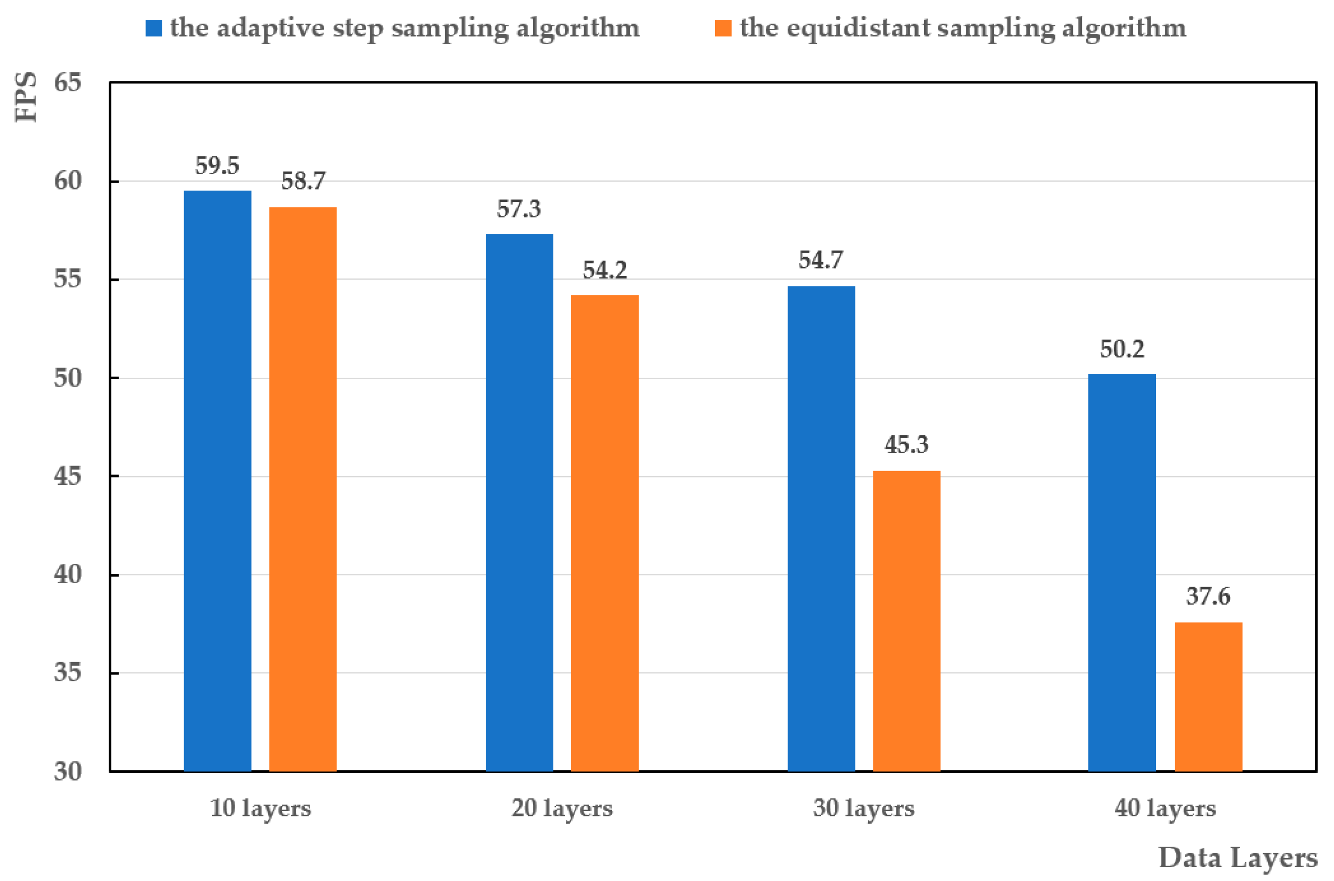
• Adaptive step-sampling algorithm: The ocean scalar field datasets are heterogeneously distributed in depth in our study. Accordingly, we construct the dataset depth identification texture. In the sampling process, first, the data level and the depth interval between the adjacent data layers are obtained according to the depth of the incident point. Then, the sampling density factor is set by calculating the data change rate of the sampling point along the optical direction, and the sampling step size is finally determined. The balance between image rendering quality and rendering efficiency is achieved by the adaptive step-sampling algorithm.
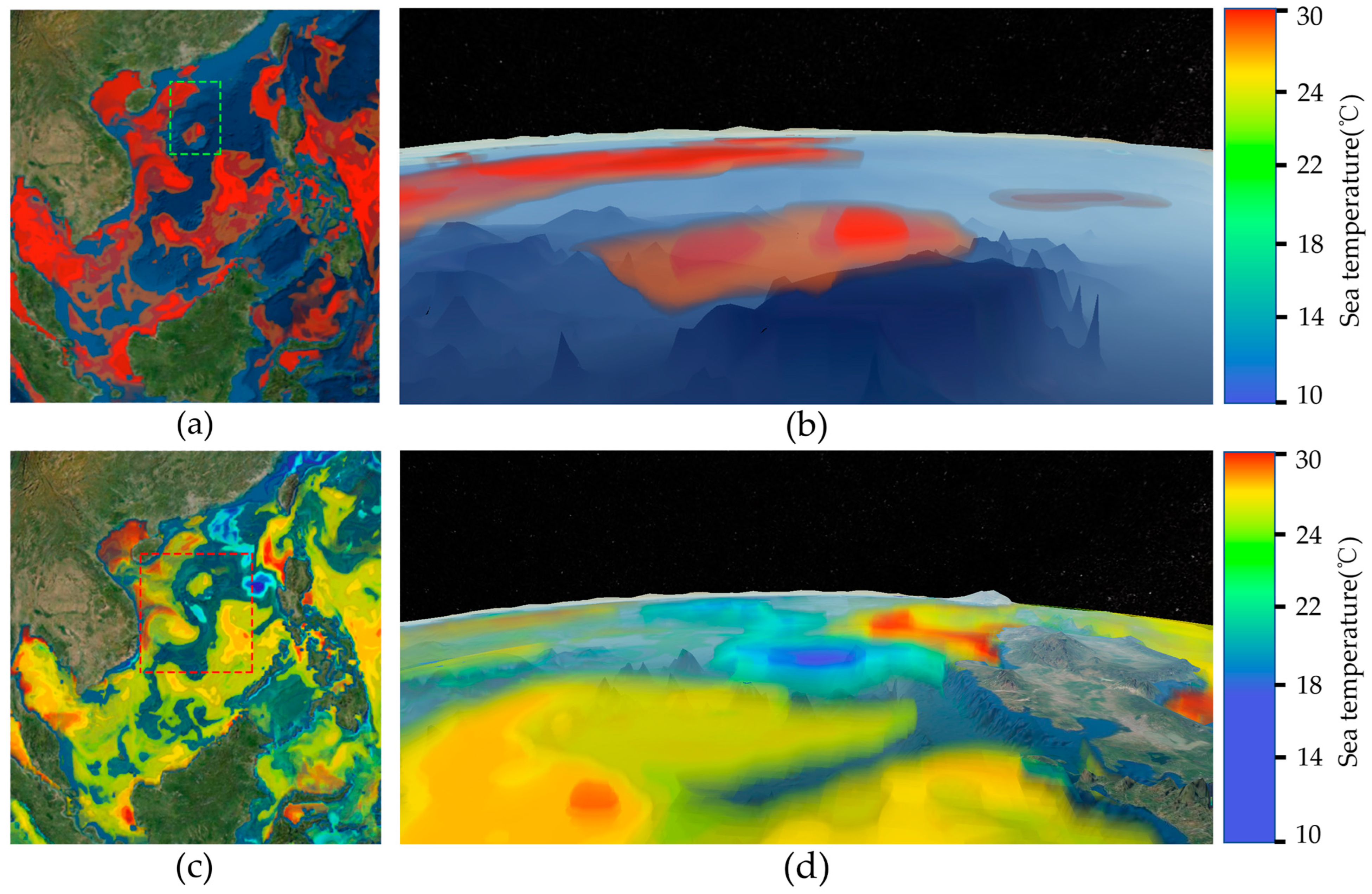
• Nonlinear color-mapping enhancement scheme: we obtain the distribution of the ocean scalar field dataset by calculating its skewness attribute and use a nonlinear color-mapping scheme to highlight the spatial distribution characteristics of the ocean scalar field. On this basis, the extraction and visualization of ocean current, vortex, and other structures and cold and hot seawater anomaly areas are realized by adjusting the transparency parameters of the transfer function.

2.2. Methodology

In this section, we discuss the spherical volume-rendering framework and terrain fusion algorithm, the adaptive step-sampling algorithm, and the color-mapping optimization scheme in detail.

2.2.1. Ocean Scalar Field Spherical Volume Rendering and Terrain Fusion

The traditional direct volume-rendering methods mostly use cubes as proxy geometry [23]. However, the proxy geometry of the cube structure cannot be close to the sphere and cannot wrap the sphere data completely in the spherical environment. At present, the double-layer spherical shell structure surrounding the globe is commonly used as the spherical proxy geometry in the spherical environment. This structure can closely wrap spatial data and achieve better visualization. However, the spatial distribution characteristics of the ocean scalar field are closely related to its actual geographical location. It will decrease the spatial accuracy when drawing the ocean volume data on the spherical surface with a ring structure. Therefore, this paper further optimizes the spherical proxy geometry to express the ocean scalar field data accurately.

The monitoring of the ocean environment in the near-shore sea area is a major focus of research in the ocean field, as it has a direct impact on the development of the ocean economy, among other things. However, the coastline of the near-shore sea area is relatively complex. The ocean scalar field grid data often cover some land at the junction of land and sea, and there is a quantity of blank grids in the land area of the volume data. If we construct the spherical proxy geometry with the data minimum enclosing rectangle directly, lots of invalid sampling points will be generated, which will decrease the computational efficiency. This paper uses the coastline vector data and the ocean scalar field data boundary to construct the minimum spatial region geometry of the study area to solve this problem.

To implement this improved proxy geometry on the sphere, the shoreline data of the study area should be edited first. The shoreline vector data is truncated with the study area data range in QGIS (a free and open-source geographic information system) software, and the obtained study area shoreline is connected with the ocean scalar field surface data vertices to construct the upper surface of the proxy geometry. Then, a spherical tessellation scheme is used to construct a proxy geometry under the sphere to enclose the volume data. Specifically, coordinates of the vertices on the upper surface are passed into the GLSL renderer. The renderer then generates triangular tessellations that approximate spherical geometry through the vertex coordinates and proxy geometry’s height. Before the actual ray-casting algorithm is executed, the entry and exit positions of each ray have to be obtained; we create two floating-point texture buffers to store them. Moreover, a GPU vertex shader and fragment shader were constructed to render the spherical bounding volume. Back-face culling and front-face culling were enabled to obtain the ray entry position and exit position. The final spherical proxy geometry is shown in Figure 2b.

This proxy geometry avoids the invalid sampling process for the land area and can significantly reduce the invalid computation. At the same time, the volume data is clipped through the sea–land vector boundary, which brings a better visualization result in the sea–land boundary area.

The calculation process of the ray-casting algorithm is carried out in GPU. In the vertex coloring system, the geographic coordinates of each voxel vertex are converted to Cartesian coordinates $(x,y,z)$ with the origin at the center of the Earth and stored in a three-dimensional array. The conversion formula is:

$$\{\begin{array}{l}x=(r-d)\cos \phi \cos \theta \\ y=(r-d)\cos \phi \sin \theta \\ z=(r-d)\sin \phi \end{array}$$

(1)

In Formula (1), $r$ is the radius of the Earth, and $d$ is the depth of the voxel vertex.

We need to convert the Cartesian coordinates of sampling points into texture coordinates $(u,v,\omega )$ to obtain the attribute values of the ocean scalar field. The texture coordinate range can be modified in the renderer to adjust the drawn content in the longitude, latitude, and depth directions in the rendering process. The coordinate transformation process is shown in Figure 3.

The marine environment is an irregular spatial data field, and the volume data of the ocean scalar field varies significantly at different depths. We usually use the trilinear spatial interpolation method to optimize the volume-rendering effect to make the color change smoother when the ray-casting algorithm is used to visualize the ocean scalar field data. Due to the large variety of data range between different depth layers of the ocean scalar field, if the lower texture data value is empty in the process of vertical interpolation, it will produce an enormous error and have a significant impact on the fusion effect of the marine environment field and the seabed terrain in the spherical environment directly using the upper data as the interpolation result. We process the seabed terrain of the study area as an image texture and load it into the GPU parallel computing pipeline to solve the above condition. The invalid sampling points under the seabed terrain are eliminated by comparing the depth value of the sampling point with the real seabed depth.

First, the Cartesian coordinates of the sampling point are obtained according to the above conversion formula. Next, we obtain the depth of the sampling point with the normalized z coordinate and the depth of the spherical proxy geometry and substitute it into the dataset depth identification texture to obtain the two data layers adjacent to sampling points and their depth intervals. Then, we use the bilinear interpolation method to smooth the data on the adjacent data layers. In this process, the distance between the sampling point and the adjacent data layer is calculated if the scalar value can be read from both adjacent data layers where the sampling point is located. The final interpolation result is obtained by inverse distance weighting. When the data value of the lower data layer of the sampling point is empty, the coordinates of the sampling point are substituted into the seabed terrain depth texture to read the actual water depth value of the position, indicated with $D_{real}$. Finally, we compare $D_{real}$ with $D_{sample}$, the depth of the sampling point. As shown in Figure 4, it retains the sampling point if $D_{sample}<D_{real}$, such as P1. Conversely, the sampling point is deleted.

2.2.2. Adaptive Step-Sampling Algorithm

The traditional ray-casting algorithm uses voxel-by-voxel sampling to ensure the accuracy of data acquisition and obtain high-quality images. For all that, it also causes a tremendous amount of computation. Virtual samplings [24] and many other methods are used to improve rendering efficiency. In this study, we proposed an adaptive step-sampling algorithm to balance the visualization effect and the rendering efficiency of the ocean scalar field according to the heterogeneous depth layers of ocean scalar field datasets.

The sampling step in ray casting should be at most 1/2 of the data layer interval in volume data to achieve a good data reconstruction result according to the Nyquist sampling law [25]. The spacing of ocean scalar field data along the depth direction is arbitrary, showing a gradually sparse distribution along the negative direction of the z-axis. In the sampling process, we create a depth identification texture according to the distribution of the depth layer of the dataset and store the data layer at the current depth and the depth interval [Sn, In] between the next layer, avoiding data redundancy caused by excessive sampling between data layers with large depth spans. The specific storage method is shown in Figure 5a. First, we obtain the coordinate of the starting point of the ray and substitute it into the depth marker texture to obtain the number of data layers and the depth interval. Then, the sampling step is calculated adaptively according to the depth interval between adjacent data layers and the sampling density factor. The sampling step increases as the depth interval enlarges, and the sampling step is calculated in the following formula.

$$Ste{p}_n=\frac{D_n}{\cos \alpha \times sf}$$

(2)

In Formula (2), $D_n$ is the depth interval between the two adjacent data layers where the sampling points are located, $\alpha$ is the angle between the ray and the vertical direction of the volume data, and $sf$ is the sampling density factor, which is used to control the sampling density of the sampling points in any depth interval. It needs to satisfy $sf\ge 2$ to ensure the quality of data reconstruction.

Meanwhile, the contribution of sampling points during the sampling process is expected to be estimated. Thus, the sampling points that rarely contribute to the final imaging are eliminated, and more detailed features of the ocean scalar field dataset are retained. In this paper, we calculate the data change rate between different data layers as the standard to judge the contribution of the sampling points, applying the depth identification texture of the ocean dataset in the sampling process. If the ray passes through the field with a large data change rate, a smaller step length is used to increase the sampling density, and the data change characteristics are restored. Otherwise, a larger fast step is used to skip and reduce invalid sampling when the light passes through the area where the data change gently. The process simulation of sea temperature change when the ray passes through the sea temperature scalar field from top to bottom is shown in Figure 6. When the light passes through the sea surface high-temperature zone and the deep low-temperature zone in the blue frame area, a smaller sampling density factor is set to reduce the redundant sampling in the constant temperature zone. Otherwise, in the red frame, where the sea temperature drops sharply, a larger sampling step is set to reduce the sampling step to keep the detailed characteristics of the seawater thermocline.

2.2.3. Nonlinear Color-Mapping Enhancement Scheme

In the ray-casting algorithm, the transfer function is defined to map the scalar value in the volume data to the color and opacity, which directly determines the imaging quality. The most commonly used method is linear color mapping, which can achieve good visualization results with evenly distributed volume data. Almost all the volume data of the ocean scalar field are unevenly distributed, which make the linear color-mapping results often concentrated in a small region of the color-mapping table. In the visualization of the ocean scalar field, more data variation characteristics, manifested as the change of color and opacity in the image, are expected to be observed. To reflect more marine environment information in the resulting image, we apply a nonlinear color-mapping method to optimize the rendering quality of the ocean scalar field.

$$V_{new}=\frac{L^{V_{raw}}-1}{L-1}$$

(3)

The nonlinear mapping function is shown in Formula (3), which will remap the normalized original attribute values of the ocean scalar field and yield the enhanced color values. Figure 7 shows the function curve when the nonlinear factor is set to 0.1 and 10.0.

The uniformity of the overall distribution of the ocean scalar dataset should be evaluated due to the need for an appropriate nonlinear factor to stretch the dataset. The skewness coefficient is the number that characterizes the asymmetry of the probability distribution density curve relative to the average value in mathematical statistics, and the skewness is often calculated using the 1st- to 3rd-order origin moments in the actual calculation. The simplified calculation formula is shown in Formula (4):

$$S(X)=E\left[{\left(\frac{X-\mu }{\sigma }\right)}^3\right]=\frac{E[X^3]-3\mu E[X^2]+2{\mu }^2}{{\sigma }^3}=\frac{E[X^3]-3\mu {\sigma }^2-{\mu }^3}{{\sigma }^3}$$

(4)

where $S(X)$ is the skewness coefficient of the dataset, $X$ is the random variable, $\mu$ is the mean value, and $\sigma$ is the standard deviation. If the skewness coefficient is 0, the data are uniformly distributed with the mean value as the dividing line. When the skewness coefficient is less than 0, we call the statistical dataset a negative deviation, and the nonlinear factor needs to be set greater than 1.0. When the skewness coefficient is greater than 0, the dataset distribution is a positive deviation, and the nonlinear factor should belong to the interval (0, 1).

3. Experiments and Results

In this section, some experiments are designed to evaluate the effect and efficiency of the spherical volume-rendering framework presented in the 3D digital Earth environment. Our visualization experiment is carried out on the cesium platform. Section 3.1 introduces the experimental datasets and the data preprocessing program. Section 3.2 compares the visualization results of the optimized proxy geometry and spatial interpolation method in this study with traditional methods. Section 3.3 analyzes the data distribution characteristics of the study area and compares the rendering image of the nonlinear color-mapping enhancement strategy and the linear mapping strategy. Section 3.4 designs the transparency transfer function to extract the typical distribution characteristics of the ocean scalar field in the study area. Section 3.5 verifies the rendering efficiency of the method proposed in this study.

3.1. Datasets and Preprocessing

3.1.1. Research Region and Datasets

The data used in this study include the ocean scalar field datasets and the seabed terrain data. We selected the Yellow Sea and the Bohai Seas of China and the South China Sea as the two research regions because our research is focused on the coastal sea area. The Yellow Sea and the Bohai Seas of China constitute a semi-open sea area, its seabed area is basically all on the continental shelf, and the depth gradually decreases from the coastline to the deep sea. Its sea area characteristics are suitable for verifying the fusion effect of the ocean scalar field and seabed terrain as a research case. The distribution and local variability of ocean environmental factors in the South China Sea are significant due to the complex topography of the seabed and the influence of the Kuroshio tributaries, so we select those two sea areas as research regions.

The ocean scalar field data mainly include ocean environmental elements, such as sea temperature, salinity, chlorophyll concentration, etc. In these elements, seawater temperature and salinity are primarily affected by solar radiation, water vapor exchange, ocean current transport, and other factors. We choose the ROMS ocean model dataset provided by the North China Sea Forecast Center of the State Oceanic Administration of China as the Yellow Sea and the Bohai Seas’ study dataset because the range of this research region is small, and the resolution of open-source data is low to meet the experimental needs. Moreover, we use the HYCOM ocean temperature and salinity dataset as the South China Sea’s study dataset [26]. Using different datasets can help us verify the adaptability of the proposed method as the output data specifications of different data models are different. The original data format is NetCDF. The details of the dataset are shown in

Table 1. Summary of the experimental datasets.

Attribute	ROMS Dataset	HYCOM Dataset
Spatial resolution	0.03° × 0.03°	0.08° × 0.08°
Time resolution	1 h	1 h
Space range	117.6° E–127.1° E, 31.9° N–41.0° N	98.8° E–130° E, −9° N–28° N
Level	11 standard vertical layers for 0–120 m	40 standard vertical layers for 0–5000 m
Dimension	287 × 274 × 11	391 × 463 × 40
Data size	3.32 Mb	19.95 Mb
DEM resolution	15 arc-second	15 arc-second
DEM data size	9.56 Mb	126.88 Mb

.

The seabed terrain data are the GEBCO_2022 grid global terrain dataset coordinated by the International Hydrographic Organization and the Intergovernmental Oceanographic Commission. Its spatial resolution is 15 arc seconds, and the measured data resolution in the equatorial region is 450 m. The spatial range of seabed terrain data is the same as that of ocean scalar field data. The data size of the terrain data is shown in Table 1.

3.1.2. Data Preprocessing

A data preprocessing program was developed to analyze and convert the original data. We used different schemes to process the data introduced above.

Data dimension reduction and color space mapping were used to convert the original three-dimensional ocean scalar datasets into two-dimensional image texture. First, each data layer in the body dataset was traversed and exported individually as a two-dimensional grid. Then, a blank picture was created with the same resolution as the dataset. The attribute values of each layer of grid points were traversed and stored in the RGB color channel of the picture pixels. The resulting two-dimensional texture image was passed into the GPU as a volume data texture. Meanwhile, a depth identification texture was created, accounting for the data layer depth distribution of the dataset. The depth identification texture has the same length with the maximum depth of the volume dataset; each depth position in the texture corresponds to the data level of the current depth in the volume dataset and the depth interval between the current layer and the next.

The seabed terrain data was processed to the sliced terrain service and a two-dimensional terrain texture. The CTB (cesium-terrain-builder) was used to generate terrain slice files and then publish them to the server. However, the scheme of real-time acquisition of seabed terrain depth through cesium lags behind and will generate a lot of data redrawing calculations. In order to judge the terrain at the sampling point in the sampling stage, we created a blank picture with the same size as the terrain. The value of the DEM was traversed and stored in the RGB color channel of the picture pixels. Then, the terrain texture was introduced into GPU for calculation.

3.2. Fusion of Ocean Scalar Field and Seabed Terrain

In this experiment, the sea temperature data of the Yellow Sea and the Bohai Sea in China were studied as the case. China’s Yellow Sea and the Bohai Sea are shallow, semi-closed coastal seas. The seabed topography of the study area is tilted from north, east and west to central and southeast [27]. The range of the sea temperature field in the study area decreases as the depth increases. The ray-casting calculation process was conducted in the GPU. The vertex coordinates of proxy geometry were introduced into the vertex shader and were bound with the digital virtual Earth by coordinate transformation, as shown in Figure 8.

Then, the ocean scalar data texture, the depth identification texture, and the seabed terrain texture were introduced into the renderer. Finally, we used the optimized ray-casting algorithm to realize the reconstruction of the ocean scalar field dataset. For comparison, we also constructed the proxy geometry of the double-layer spherical shell structure used by Liang and Zhang et al. and used the conventional trilinear interpolation method to obtain the attribute values at the sampling points. The rendering result is shown in Figure 9a. Figure 9b is the rendering result of using the proposed minimum bounding volume structure as the proxy geometry and introducing the seabed terrain texture for depth judgment. We can find that before applying the seabed terrain texture, as shown in the red border area in Figure 9a, there are apparent data range jumps between different depth levels, and the cross-section transitions show a ladder shape. Moreover, the coastal terrain changes cannot be observed, and the geomorphological features are covered entirely, as shown in Figure 9a. After being optimized with the method in this study, the transition between different depth layers becomes smooth, and the fusion effect of the ocean scalar field and seafloor topography is significantly improved in the red border area in Figure 9b. In addition, we found the geomorphic features of underwater dunes along the Yellow Sea coast of China and the topographic changes at the land–sea junction of the Korean Peninsula. This experiment illustrates the improved spherical proxy geometric model, and the optimized spatial interpolation algorithm with depth judgment can significantly strengthen the expression of the ocean scalar field in the nearshore and bay areas.

3.3. Nonlinear Color Mapping

Seawater temperature is a physical quantity that characterizes the thermal condition of seawater. Solar radiation and ocean–atmosphere heat exchange are the two main factors affecting seawater temperature [28]. In addition, the current also significantly affects the seawater temperature in local sea areas. The surface seawater temperature decreases with depth, and the change within 1000 m is more prominent. In the range of 100–200 m of seawater, there is a layer with a sharp decrease in sea temperature between the thin warm water layer on the sea surface and the thick cold water layer below, which is called the thermocline, one of the critical phenomena in oceanographic research. The distribution of salinity in the open sea is relatively uniform, mainly impacted by ocean currents. Another factor affecting salinity is freshwater inflow, which mainly occurs in the estuaries of rivers. We chose the study area of the South China Sea and its surrounding waters, where the distribution of the ocean scalar field is affected by the Kuroshio tributaries. The temperature and salinity activities are more active in the ocean surface layer. Considering the above factors, our study concentrates on the sea temperature and salinity field in the range of 0–300 m in the South China Sea and its surrounding waters. We obtained the data distribution frequency statistical graph and the dataset’s skewness through statistical data analysis. In Figure 10, the red and green vertical lines represent the position of the median and average of the dataset in the histogram, respectively. We used the 1st to 3rd-order origin moments to calculate the skewness of the sea temperature dataset and the salinity dataset in the study area, which are −1.64 and −3.0. The distribution of seawater temperature and salinity in the study area has prominent negative skewness characteristics.

Because the sea temperature and salinity fields in the research region show a negatively skewed distribution, the nonlinear factors should be greater than 1.0. We finally adopted 4.0 and 6.0 as the nonlinear factors to stretch the original attribute values of sea temperature and salinity field and perform the color-mapping function. As shown in Figure 11a,c, in the case of linear color mapping, the color distribution of volume-rendering images is concentrated in a small color range, and the details of the spatial distribution characteristics of the ocean scalar field are lost. Figure 11b,d show the image enhanced by nonlinear mapping. Compared with the results of linear mappings, the volume-rendering result image is stretched to more color ranges. It reveals more spatial distribution characteristics of sea temperature and salinity field by color variation.

3.4. Ocean Three-Dimensional Feature Structure Extraction

The transfer function is the most critical part of the ray-casting algorithm. We can use the nonlinear color-mapping strategy to enhance the overall effect of the ocean scalar field volume rendering in our transfer function construction process. Moreover, the appropriately designed transfer function can realize the extraction of the local feature structure of the study areas. Regions of interest in ocean scalar field data are given low transparency, and other non-concerned regions can be displayed in translucent or even full transparency.

Seawater temperature gradually decreases from low latitudes to high latitudes in most cases. In local sea areas, the changes in sea temperature and salinity are affected by seawater movement. Ocean currents and vortexes can cause an anomalous regional distribution of sea temperature and salinity. The South China Sea and its surrounding waters are affected by the Kuroshio Branch Current [29]. The mesoscale vortex shedding from the Kuroshio Branch Current will cause local thermal anomalies in this area. In this study, we designed two experiments to achieve the extraction of regional sea surface temperature anomalies in the research area. We can observe the temperature changes caused by ocean currents and vortices in the images enhanced by the nonlinear color-mapping scheme, providing a reference for the transparency transfer function’s design. In the first experiment, we set low transparency to the sea temperature in the interval of [0.9,1.0] and made the data of other intervals transparent. Thus, we realized the extraction of local heat water masses in the study area, as shown in Figure 12. In another experiment, we assigned a lower transparency to sea temperature values in the intervals [0.2,0.3] and [0.6,0.9] and a higher transparency to the other intervals, achieving the extraction of the regions of intensely hot and cold variations in the study area, which is shown in Figure 12.

The surface salinity generally increases with sea depth in the South China Sea and its surrounding waters. In addition, ocean currents, vortex, and coastal freshwater injection also have an important impact on the salinity changes in the study area. The northwest coastal area of the Gulf of Thailand in the study area is fed by many rivers, and there is a seasonal circulation in the Gulf, resulting in significant variation in salinity in the Gulf of Thailand [30]. We designed two experiments to extract the current structure in the study area and the salinity change structure in the Gulf of Thailand according to the distribution characteristics of the salinity field in the study area. First, we set the normalized scalar value in [0.4,0.7] to the low transparency and the rest to the high transparency to obtain the ocean current structure extraction image of the study area, as shown in Figure 13a,b. The characteristics of sea surface salinity variation caused by ocean current disturbance is significant. In addition, we used a color band with a broader range and concentrated the function mapping interval in the salinity range in the Gulf of Thailand. The salinity variation structure extraction of the Gulf of Thailand and surrounding areas was obtained by setting the transparency of the normalized salinity in the interval [0.95,1] to 1.0. The spatial distribution characteristics of salinity caused by freshwater inflow and circulation in the Gulf of Thailand can be observed in Figure 13d.

3.5. Rendering Efficiency Test

We designed an experiment to evaluate the performance of the proposed method, using FPS (frames per second) as the measuring standard of rendering efficiency. The client machine has 16 GB memory, Inter Core i5-12490F operating at 2.3 GHz, and an NVIDIA GeForce TRX 2060 GPU.

The first experiment verified the performance of the proposed method by testing the frame rate of two experimental datasets in the interactive state. Figure 14 shows the average frame rate of the two datasets used in this study under different sampling density factor settings. DataSet1 is the sea temperature dataset of the Yellow Sea and Bohai Sea in China, and DataSet2 is the sea temperature dataset of the South China Sea and its surrounding areas.

Moreover, in order to test the efficiency of the adaptive step-sampling algorithm proposed in this paper, we used the equidistant sampling algorithm as a comparison experiment. The frame rate test was performed on the first 10 layers, 20 layers, 30 layers, and 40 layers of DataSet2. The experimental results are shown in Figure 15.

4. Discussion

4.1. Visualization Effect Analysis

In Section 3, we designed two sets of comparative experiments to verify the improvement of the visualization effect of the research method proposed in this paper, and on this basis, some typical oceanic phenomena in the study area were visualized.

According to the results in Section 3.2, the method proposed in this paper greatly improved the accuracy of three-dimensional visualization and the fusion effect with seabed terrain compared with the methods in References [19,20] in the three-dimensional visualization of ocean scalar field in coastal waters.

By comparing the rendering results in Figure 11, the nonlinear color-mapping scheme based on the skewness of the dataset solves the problem of missing local details of the ocean scalar field caused by the over-concentration of the mapping results in the case of uneven data distribution. Researchers can find more spatial distribution characteristics and variation rules of the ocean scalar field. On this basis, we realized the extraction of typical ocean phenomena, such as sea temperature anomalies and ocean currents, by adjusting the transfer function, which further demonstrates the advantages and scalability of our method in studying ocean scalar fields.

4.2. Performance Analysis

In Section 3.5, two experiments were designed to test the performance of the proposed visualization method.

Figure 14 shows that the average frame rate decreases with the increase of sampling density factor and volume data volume. The frame rates of the two datasets were 50.3 and 35.4 when the sampling density factor was set to 20. The sampling density factor was generally less than 10 in rendering. The lowest coherent picture the human eye can accept is 24 frames per second. A smooth effect can be achieved when the frame rate is greater than 30. Therefore, the rendering images of the two datasets can maintain a smooth visualization effect in the interactive state.

In Figure 15, the adaptive sampling algorithm is slightly better than the equidistant sampling algorithm in the frame rate test when the data layers is set to 10 and 20. As the data layers increase, the adaptive step size algorithm shows obvious efficiency compared to the equidistant sampling algorithm because the latter will generate a large amount of redundant sampling between data layers with large depth intervals.

5. Conclusions and Prospects

This paper proposes a spherical volume-rendering method of ocean scalar field based on the ray-casting algorithm in the virtual Earth environment, and the accuracy and efficiency of volume rendering of the ocean scalar field in a spherical environment are improved. The contribution and conclusions of this study are as follows:

• First, a new spherical proxy geometry using the minimum bounding volume was proposed, and the seabed terrain depth texture was introduced into the spatial interpolation process. Thus, we improved the visualization effect of the ocean scalar field at the junction of land and sea and realized the fusion of three-dimensional reconstruction results of the ocean scalar field and seabed topography.
• Second, we proposed an adaptive step-sampling algorithm based on heterogeneous depth layer and data change rate of ocean scalar field datasets, which achieves a balance between the ray-casting effect and rendering efficiency.
• Third, we calculated the skewness as the standard to measure the deviation degree of the dataset and applied a nonlinear color-mapping scheme to enhance the effect of volume rendering. Combined with the transparency transfer function, the spatial distribution of the ocean scalar field was highlighted and some typical ocean phenomena were analyzed, which demonstrate the advantages and scalability of our method in studying ocean scalar fields.

However, since our research was focused on the near-shore ocean scalar field, the visualization method proposed in this paper also has its weaknesses and limitations. First, the efficiency improvement is not obvious when the dataset depth interval distribution is more uniform. Moreover, a limitation of the method is it can only be used for visualizing small- and medium-scale coastal sea areas.

In future research, we will expand the research area, realize the fusion of ocean scalar field and terrain at the global scale, and extract more structural features of typical ocean movements and phenomena. In addition, we will build a temporal digital Earth framework that supports dynamic visualization of long-time ocean phenomena.

References

1. McCormick, B.H.; DeFanti, T.A.; Brown, M.D. Visualization in Scientific Computing-A Synopsis. IEEE Comput. Graph. Appl. 1987, 7, 61–70. [Google Scholar] [CrossRef]
2. Liu, S.; Chen, G.; Yao, S.; Tian, F.; Liu, W. A framework for interactive visual analysis of heterogeneous marine data in an integrated problem solving environment. Comput. Geosci. 2017, 104, 20–28. [Google Scholar] [CrossRef]
3. Lorensen, W.E.; Cline, H.E. Marching cubes: A high resolution 3D surface construction algorithm. Siggraph Comput. Graph. 1987, 21, 163–169. [Google Scholar] [CrossRef]
4. Max, N. Optical models for direct volume rendering. IEEE Trans. Vis. Comput. Graph. 1995, 1, 99–108. [Google Scholar] [CrossRef] [Green Version]
5. Westover, L. Footprint evaluation for volume rendering. In Proceedings of the 17th Annual Conference on Computer Graphics and Interactive Techniques, Dallas, TX, USA, 6–10 August 1990; pp. 367–376. [Google Scholar]
6. Hon, T.C.; Rangayyan, R.M.; Hahn, L.J.; Kloiber, R. Three-dimensional display in nuclear medicine. IEEE Trans. Med. Imaging 1989, 8, 297–330. [Google Scholar]
7. Lacroute, P.; Levoy, M. Fast volume rendering using a shear-warp factorization of the viewing transformation. In Proceedings of the 21st Annual Conference on Computer Graphics and Interactive Techniques, Orlando, FL, USA, 24–29 July 1994; pp. 451–458. [Google Scholar] [CrossRef] [Green Version]
8. Levoy, M. Display of surfaces from volume data. Comput. Graph. Appl. 1988, 8, 29–37. [Google Scholar] [CrossRef] [Green Version]
9. Engel, K.; Kraus, M.; Ertl, T. High-quality pre-integrated volume rendering using hardware-accelerated pixel shading. In Proceedings of the ACM SIGGRAPH/EUROGRAPHICS Workshop on Graphics Hardware (HWWS’01); Association for Computing Machinery: New York, NY, USA, 2001; pp. 9–16. [Google Scholar] [CrossRef]
10. Kruger, J.; Westermann, R. Acceleration techniques for GPU-based volume rendering. In Proceedings of the IEEE Visualization, 2003. VIS 2003, Seattle, WA, USA, 19–24 October 2003. [Google Scholar]
11. Pfister, H.; Lorensen, B.; Bajaj, C.; Kindlmann, G.; Schroeder, W.; Avila, L.S.; Raghu, K.M.; Machiraju, R.; Lee, J. The transfer function bake-off. IEEE Comput. Graph. Appl. 2001, 21, 16–22. [Google Scholar] [CrossRef]
12. Correa, C.D.; Ma, K.L. Visibility-driven transfer functions. In Proceedings of the IEEE Pacific Visualization Symposium, Beijing, China, 20–23 April 2009. [Google Scholar]
13. Wang, Y.; Zhang, J.; Chen, W.; Zhang, H.; Chi, X. Efficient opacity specification based on feature visibilities in direct volume rendering. Comput. Graph. Forum 2011, 30, 2117–2126. [Google Scholar] [CrossRef]
14. Ruiz, M.; Bardera, A.; Boada, I.; Viola, I.; Feixas, M.; Sbert, M. Automatic Transfer Functions Based on Informational Divergence. IEEE Trans. Vis. Comput. Graph. 2011, 17, 1932–1941. [Google Scholar] [CrossRef] [Green Version]
15. Deakin, L.J.; Knackstedt, M.A. Efficient ray casting of volumetric images using distance maps for empty space skipping. Comput. Vis. Media 2020, 6, 53–63. [Google Scholar] [CrossRef] [Green Version]
16. Feng, Y.; Han, B. Ocean Temperature Field 3D Visualization Key Technology Research Based on Pseudo-octree Model. J. Phys. Conf. Ser. 2018, 1064, 012064. [Google Scholar] [CrossRef]
17. Li, J.; Wu, H.; Yang, C.; Wong, D.W.; Xie, J. Visualizing dynamic geosciences phenomena using an octree-based view-dependent LOD strategy within virtual globes. Comput. Geosci. 2011, 37, 1295–1302. [Google Scholar] [CrossRef]
18. Liu, P.; Gong, J.; Yu, M. Graphics processing unit-based dynamic volume rendering for typhoons on a virtual globe. Int. J. Digit. Earth 2015, 8, 431–450. [Google Scholar] [CrossRef]
19. Liang, J.; Gong, J.; Li, W.; Ibrahim, A.N. Visualizing 3D atmospheric data with spherical volume texture on virtual globes. Comput. Geosci. 2014, 68, 81–91. [Google Scholar] [CrossRef]
20. Zhang, X.; Yue, P.; Chen, Y.; Hu, L. An efficient dynamic volume rendering for large-scale meteorological data in a virtual globe. Comput. Geosci. 2019, 126, 1–8. [Google Scholar] [CrossRef]
21. Li, W.; Wang, S. PolarGlobe: A web-wide virtual globe system for visualizing multidimensional, time-varying, big climate data. Int. J. Geogr. Inf. Sci. 2017, 31, 1562–1582. [Google Scholar] [CrossRef]
22. Qin, R.; Feng, B.; Xu, Z.; Zhou, Y.; Liu, L.; Li, Y. Web-based 3D visualization framework for time-varying and large-volume oceanic forecasting data using open-source technologies. Environ. Model. Softw. 2021, 135, 104908. [Google Scholar] [CrossRef]
23. Rautenhaus, M.; Bottinger, M.; Siemen, S.; Hoffman, R.; Kirby, R.M.; Mirzargar, M.; Rober, N.; Westermann, R. Visualization in Meteorology—A Survey of Techniques and Tools for Data Analysis Tasks. IEEE Trans. Vis. Comput. Graph. 2018, 24, 3268–3296. [Google Scholar] [CrossRef]
24. Lee, B.; Yun, J.; Seo, J.; Shim, B.; Shin, Y.-G.; Kim, B. Fast High-Quality Volume Ray Casting with Virtual Samplings. IEEE Trans. Vis. Comput. Graph. 2010, 16, 1525–1532. [Google Scholar] [CrossRef]
25. Nyquist, H. Certain Topics in Telegraph Transmission Theory. Trans. Am. Inst. Electr. Eng. 1928, 47, 617–644. [Google Scholar] [CrossRef]
26. Wallcraft, A.; Carroll, S.; Kelly, K.; Rushing, K. Hybrid Coordinate Ocean Model (HYCOM) Version 2.1. User’s Guide. Hybrid Coordinate Ocean Model Version.Users Guide 2003. Available online: https://www.hycom.org/hycom/documentation/63-hycom-users-manual-and-guide (accessed on 8 May 2009).
27. Zeng, X.; He, R.; Xue, Z.; Wang, H.; Wang, Y.; Yao, Z.; Guan, W.; Warrillow, J. River-derived sediment suspension and transport in the Bohai, Yellow, and East China Seas: A preliminary modeling study. Cont. Shelf Res. 2015, 111, 112–125. [Google Scholar] [CrossRef] [Green Version]
28. Liang, X.; Wu, L. Effects of solar penetration on the annual cycle of sea surface temperature in the North Pacific. J. Geophys. Res. Oceans 2013, 118, 2793–2801. [Google Scholar] [CrossRef]
29. Feng, N.; Xue, H.; Fei, Y. Kuroshio intrusion into the South China Sea: A review. Prog. Oceanogr. 2015, 137, 314–333. [Google Scholar]
30. Aschariyaphotha, N.; Wongwises, S. Simulations of Seasonal Current Circulations and Its Variabilities Forced by Runoff from Freshwater in the Gulf of Thailand. Arab. J. Sci. Eng. 2012, 37, 1389–1404. [Google Scholar] [CrossRef]
Figure 1. Ocean scalar field volume-rendering research framework in a spherical environment.
Ijgi 12 00153 g001
Figure 2. Spherical agent geometry contrast figure: (a) double spherical shell bounding box structure; (b) minimum bounding volume structure based on the spherical inlay.
Ijgi 12 00153 g002
Figure 3. (a) Conversion of geographical coordinates to Cartesian coordinates; (b) obtained texture coordinates according to Cartesian coordinates.
Ijgi 12 00153 g003
Figure 4. (a) Multi-profile data of ocean scalar field in the study area; (b) the depth judgment diagram in spatial interpolation in which blue planes represent the adjacent data layer of sampling points, and the purple surface represents seabed terrain; (c) seabed terrain of the study area.
Ijgi 12 00153 g004
Figure 5. (a) Ocean scalar field-depth identification texture; the sampling point’s data levels are stored in the R channel, and the interval to the following data level is stored in the G channel and B channel; (b) schematic diagram of adjusting sampling step size according to data layer depth interval.
Ijgi 12 00153 g005
Figure 6. Adjustment of the sampling density factor according to the data change rate.
Ijgi 12 00153 g006
Figure 7. Nonlinear mapping function curve. The black line represents the linear mapping image, and the red and blue lines represent the nonlinear mapping function image when the nonlinearity factor is set to 0.1 and 10.0.
Ijgi 12 00153 g007
Figure 8. Spherical proxy geometry in the Yellow Sea and Bohai Sea research area of China.
Ijgi 12 00153 g008
Figure 9. On the left, (a) is the rendering result of using a double-layer spherical shell structure proxy geometry and the traditional trilinear interpolation method; (b) is the rendering result of using the proposed minimum bounding volume structure as the proxy geometry and introducing the seabed terrain texture for depth judgment.
Ijgi 12 00153 g009
Figure 10. Above, (a,b) are the statistical histogram of sea temperature and salinity field datasets in the experimental area; the data range is 98.8° E–130° E, −9° N–28° N.
Ijgi 12 00153 g010
Figure 11. (a) Comparison of linear color mapping and nonlinear color mapping: (a,c) are the images of linear color mapping of sea temperature and salinity field, (b,d) are the images enhanced by the nonlinear color-mapping method.
Ijgi 12 00153 g011
Figure 12. Above, (a,b) are the feature extraction visualizations of the hot zone in the study area; (c,d) show the local sea temperature anomaly caused by seawater movement.
Ijgi 12 00153 g012
Figure 13. Above, (a,b) are the feature extraction visualization of ocean current in the study area; (c,d) show the characteristics of salinity variation structure in the Gulf of Thailand.
Ijgi 12 00153 g013
Figure 14. Ocean scalar field volume-rendering performance with different sampling density.
Ijgi 12 00153 g014
Figure 15. The frame rate comparison diagram of the adaptive step-sampling algorithm and the equidistant sampling algorithm in the interactive stat.
Ijgi 12 00153 g015