Assessing Completeness of OpenStreetMap Building Footprints Using MapSwipe

Abstract

Natural hazards threaten millions of people all over the world. To address this risk, exposure and vulnerability models with high resolution data are essential. However, in many areas of the world, exposure models are rather coarse and are aggregated over large areas. Although OpenStreetMap (OSM) offers great potential to assess risk at a detailed building-by-building level, the completeness of OSM building footprints is still heterogeneous. We present an approach to close this gap by means of crowd-sourcing based on the mobile app MapSwipe, where volunteers swipe through satellite images of a region collecting user feedback on classification tasks. For our application, MapSwipe was extended by a completeness feature that allows to classify a tile as “no building”, “complete” or “incomplete”. To assess the quality of the produced data, the completeness feature was applied to four regions. The MapSwipe-based assessment was compared with an intrinsic approach to quantify completeness and with the prediction of an existing model. Our results show that the crowd-sourced approach yields a reasonable classification performance of the completeness of OSM building footprints. Results showed that the MapSwipe-based assessment produced consistent estimates for the case study regions while the other two approaches showed a higher variability. Our study also revealed that volunteers tend to classify nearly completely mapped tiles as “complete”, especially in areas with a high OSM building density. Another factor that influenced the classification performance was the level of alignment of the OSM layer with the satellite imagery.

1. Introduction

Natural hazards such as earthquakes, floods and tornadoes threaten millions of people all over the world [1]. The effects of these hazards on society and infrastructure depend on the vulnerability towards the hazards [2]. These vulnerabilities are highly dynamic as some are decreasing due to new building codes, preparedness actions and resilient planning, while others are increasing due to rapid urbanization, increased industrialization, aging infrastructure and stronger interdependencies in modern societies [3,4]. Regardless of the different hazards or even combinations of them, it is key for emergency planning, resilience building and first response to catastrophes to understand the risks that a society is exposed to. Because risk is the combination of hazard, exposure and vulnerability, all three aspects of the risk chain need to be well understood for any measure to be taken to reduce it [5].

In this paper, we focus on the exposure part of the risk chain. Exposure models, describing the spatial distribution of assets (usually buildings and people) and the relative distribution of different building types, show different levels of resolution and precision [6]. In well-regulated countries, such models may describe the location of each building. In high-resolution studies, each building may be individually described in all relevant parameters. However, in many areas of the world, exposure models are rather coarse and are aggregated over large areas, sometimes even over entire countries. This results in them being useful only if the damage or losses are estimated at this aggregation level too. To address local planning or local emergency response, exposure models with high resolution down to the building scale are desired. To create exposure models on the building scale, the location and additional parameters of the buildings such as the building footprint, building height and building material need to be known. This information is usually provided by cadastral data. However, such data is not available everywhere, either because its use is restricted, expensive or it does not even exist [7].

The free and open geographic data community project OpenStreetMap (OSM) is potentially able to fill this gap. Although OSM data have been used extensively in disaster mapping and management [8], their completeness is heterogeneous, with some areas very well mapped and other areas lacking basic features [9,10,11]. For example, the completeness of highly populated urban areas is often higher than that of remote and rural areas [10,12]. There are also differences between developed and developing countries [11,13]. These disparities depend on social factors, such as population distribution and population density, as well as the location of contributing users [14].

Therefore, the assessment of the spatially heterogeneous data quality in OSM is of great importance. Current approaches can be distinguished mainly in extrinsic and intrinsic approaches. Extrinsic approaches use reference datasets as a benchmark to compare OSM against using indicators such as the length of the road network or the number of buildings or the positional accuracy of features such as buildings [10,15,16]. These approaches face the challenge of missing reference data of sufficient quality, especially for large parts of the global South. For building footprints Biljecki et al. [17] provide an overview about available administrative data. Object detection by deep learning approaches seems promising to provide reference data for OSM objects. For land-cover OSM objects, Schott et al. [18] demonstrated the potential of noise-robust deep-learning approaches used on satellite imagery to detect potential errors in OSM land-use information. For building footprints, datasets such as the Microsoft building footprints layer [19] are a potential reference for an increasing—but still limited—number of countries and have been used to assess the completeness of building footprints for 13,189 urban agglomerations by fitting a machine learning model to them [13]. Research by Herfort et al. [13] has shown that crowd-sourcing approaches, such as the one presented here, and deep-learning approaches might complement each other.

Even if reference data are available, it might be less current than OSM and cover only a subset of the relevant features [20]. To overcome these issues, intrinsic approaches have been developed which address different aspects of data quality only based on the historical development of OSM [21,22,23,24]. Completeness of map features is thereby, for example, addressed by fitting saturation curves to the OSM contribution time series to assess the difference between fitted asymptote and current number of objects [12] or by deriving community activity stages [25,26]. The completeness assessment based on saturation curves can only be used for areas with a reasonably high number of OSM features. Other approaches have tried to estimate the expected number of objects based on covariates, such as building density or geometric indicators at street-block level to estimate building completeness [27,28], socioeconomic indicators, population density or urban–rural gradients [12,29,30]. Given large regional differences in both real-world features (such as building density) and mapping activity, the latter approaches are limited with respect to their transferability between regions, especially across urban–rural gradients or cultural boundaries. Schott et al. [31] have implemented and tested a set of 32 intrinsic and semi-intrinsic indicators for different aspects of data quality. While they tested for land-use- and land-cover-related feature classes, many indicators are presumably transferable to other domains such as building footprints.

The Humanitarian OpenStreetMap Team (HOT) [32] and other humanitarian organizations have been addressing the issue of OSM data completeness since 2010 by activating volunteers to map buildings and roads. HOT stimulated volunteers through mostly catastrophe-related activities in collaboration with first responders in need of good maps with building locations. This imminent benefit of the volunteers’ work for first responders has certainly drawn a lot of attention to humanitarian mapping activities in OSM. However, HOT and other organizations have not limited their activities to ongoing or imminent catastrophes, but expanded them to mapping larger areas [11,14]. This led to the missing maps network that aims to move from reaction to action, putting vulnerable areas/people on the map before the next disaster hits [33].

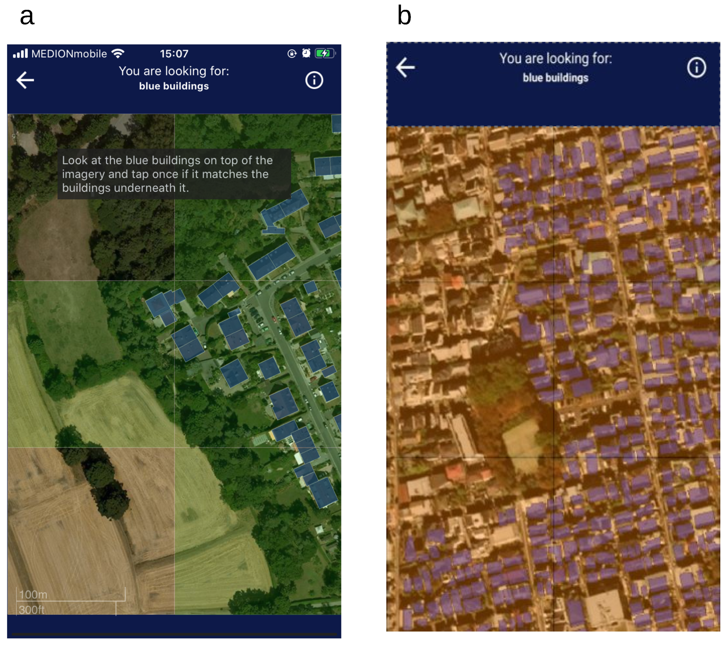
While a lot of resources and tools are in place to ease mapping in OSM, some learning effort is still needed for newcomers wanting to contribute. To ease that initial hurdle, the smartphone application MapSwipe [34] has been designed as a tool that requires only a minimum training effort and that uses a simple and easy-to-learn user interface. The tool has been developed and is maintained by the Heidelberg Institute for Geoinformation Technology (HeiGIT) in cooperation with the British Red Cross (BRC), the Humanitarian OpenStreetMap Team (HOT), Médecins Sans Frontières (MSF) and volunteers. MapSwipe introduced the aspect of gamification to the detection of buildings by showing the user satellite imagery prompting for the selection of areas in which buildings can be identified by the user [35]. Once these areas are marked, the user swipes the satellite imagery aside to receive the next images—hence the name MapSwipe.

The images are categorized into groups: those with buildings and those without buildings. This process simplifies the task of digitizing the building footprints for OSM contributors, as they no longer have to scan through the entire area for buildings. This pre-selection of areas for mapping activities has proven useful as nearly 50,000 MapSwipe users have mapped more than 1,750,000 sqkm and finished about 500 projects. The data are publicly available for further use [36]. The HOT activities, together with MapSwipe as well as regular OSM volunteer mapping, have made data in OSM become a ubiquitous part of disaster planning, emergency management and first response [37]. The intended target group for MapSwipe has been users that lack experience in mapping in the OSM ecosystem. Therefore, the app was designed to require only a minimum training effort, which is reflected in an easy-to-learn user interface.

MapSwipe conceptually extends desktop-based approaches such as Tomnod to the smartphone, thereby further lowering the bar for volunteers by enabling them to contribute easily during idle periods such as while riding a subway or waiting for a bus. Tomnod—a former project of the satellite company DigitalGlobe—was known for its campaigns such as searching for the missing Malaysian Airlines flight MH370, which attracted over eight million participants [38] before being discontinued in August 2019.

Gamification in MapSwipe was implemented by experience points the users obtain for completed tasks which are reflected in experience levels through the badges gained. This simple approach has been frequently used for crowd-sourcing applications with relatively simple repetitive tasks [39]. The user-level information about MapSwipe activity accessible for registered users is comparable to other approaches in the OSM ecosystem such as for the HOT tasking manager or “How did you contribute to OSM?” [40]. User level comparison such as those implemented for OSM users by “OSMFight” [41] was not implemented at the time of writing.

Because risk assessment models that use OSM data also have to address the spatially varying completeness, it is important to identify areas with complete OSM building footprints for which detailed exposure models can be provided. Furthermore, emergency groups can plan additional mapping efforts in unmapped areas that are particularly affected by natural catastrophes. In contrast to the previous MapSwipe project types that are used to provide information about the presence or absence of buildings on satellite imagery, we introduced a completeness project type that classifies areas with regard to the completeness of OSM building footprints. This is intended to steer mapping activities of volunteers, for example in the HOT tasking manger, to areas where information is missing for activities such as disaster response or forecast-based financing. The new project type was designed with the intended target group of unexperienced users in mind. Therefore, the design was kept simple at the cost of limited user input options.

This study aims at investigating the robustness of the completeness data produced by this crowd-sourced approach and aims to examine the following specific research questions:

1.

What factors influence the performance of the OSM building completeness classification?

2.

How well can the completeness feature produce reliable results so that it can be used in applications of risk-assessment solutions, such as exposure modeling?

3.

How well can building completeness be captured by the MapSwipe approach compared to existing approaches?

The new completeness feature in the MapSwipe application is part of a larger project. The Heidelberg University, the German Research Centre for Geosciences (GFZ) in Potsdam, the Karlsruhe Institute of Technology (KIT), the Research Center for Information Technology (FZI) in Karlsruhe and the company Aeromey GmbH have teamed up in the project LOKI (Airborne Observation of Critical Infrastructures) to deliver a system based on OSM data for rapid damage assessment after earthquakes using a variety of technologies including unmanned aerial vehicles (UAV), machine learning, crowd-sourcing for recording the disaster scene and exposure models at the building scale. LOKI combines in an interdisciplinary way new technologies with existing expertise in earthquake research and earthquake-engineering knowledge [42]. In this light, the completeness feature from MapSwipe aims to increase the resolution of existing exposure models from aggregated exposure information to a detailed building-by-building description, and to identify areas where further mapping effort is required.

2. MapSwipe Data Model

MapSwipe is a mobile application that was developed within the Missing Maps project in 2014 [34]. Generally, the app comprises four important concepts: projects, groups, tasks and results. A project describes a region of interest. Based on the defined region, satellite imagery tiles are requested from a specific imagery provider. While creating the project, the project name, a project image, a zoom level (usually zoom level 18, extending approx. 150 m in equatorial areas and about 100 m in central Europe), and the number of users that are requested to verify a single tile, can be defined. The MapSwipe tasks correspond to the satellite imagery at the specified zoom level. Other parameter such as metadata about the map provider can also be specified.

Regarding the completeness feature, each task is associated with a satellite imagery tile from Bing Maps with a semi-transparent overlay of the OSM building footprints. The mobile app, representing the client, requests these tasks from the database. In order to enable a fast and efficient communication between the client and the database, groups have been introduced to reduce the amount of client requests. Each group consists of several tasks, which compose one mapping session. Results contain information on the user classification. A single classification result comprises information about the task ID, task geometry and tile classification. For the completeness feature project type, volunteers have to classify the completeness of each task into one of three categories: “no building” (no tap), “complete” (one tap) or “incomplete” (two taps). The classification is conducted by tapping on each tile; tapping loops through the three options. The main screen of the app is divided into six tasks (cf. Figure 1). A tile is considered complete if the blue colored OSM building footprints cover all the buildings in the satellite imagery. Conversely, if the OSM building footprint does not cover all buildings visible in the imagery, the tile is regarded as incomplete. In case of no buildings are present in the satellite imagery, there is no need to tap and the user can swipe to the next screen, hereby indicating that the tile does not contain any buildings. Additionally, the users are aided in the tasks by a brief tutorial. The results of the volunteers can be obtained from the MapSwipeDev-API [43].

3. Case Study

In our case study, we investigated building completeness at four study sites (cf. Figure 2): Siros, Taipei, Tokyo and Medellin. These sites comprise heterogeneous OSM building coverage, including fully complete areas as well as incomplete areas. The four sites cover an overall area of 89.3 sqkm subdivided into 4797 tasks (cf.

Table 1. Characterization of the MapSwipe projects used as case study sites for the assessment of building completeness. For the average number of buildings and the average building footprint area per task area, the standard deviation is provided in parenthesis.

Name	Area [sqkm]	Tasks	OSM Building Coverage	Number of OSM Buildings per Task [1/ha]	OSM Building Footprint Area per Task [%]
Tokyo	27.5	1914	Urban area including fully mapped, partly mapped and unmapped areas	23.6 (24.4)	21.0 (17.8)
Taipei	13.7	792	Urban area including fully mapped, partly mapped and unmapped areas	3.6 (5.2)	11.5 (15.2)
Siros	25.0	981	Island accompanied by smaller patches of agricultural land including fully mapped and partly mapped areas	7.1 (15.3)	5.7 (11.4)
Medellin	23.1	1110	Northern part including high building density with almost completely mapped areas, less densely populated southern part consisting of single-family homes with partly mapped areas	4.8 (8.0)	13.4 (16.3)
Total	89.3	4797

). Multiple sites were selected as the varying building shapes, building sizes, building roof textures, as well as different land-cover settings (e.g., trees overlapping buildings) allow for the assessment of the classification behavior of the volunteers in different geographical settings.

In order to create a project in MapSwipe, all four sites were combined into one area of interest. After the project creation, a completeness mapping event was organized on 16 September 2020. Nine participants with different levels of experience took part in the project to evaluate the completeness of OSM building footprints. On average, a participant required 0.38 s per task with an interquartile range of 0.1 s.

4. Materials and Methods

4.1. Data

All participants collected completeness-classification data during our mapping event using MapSwipe on their smartphones. Each task was assessed by at least five of the nine volunteers. To validate the crowd-sourced classification results, the data were compared to a reference dataset. For the reference data, three experts from the LOKI project classified each task carefully, resulting in three expert classifications per task.

4.2. Data Pre-Processing

Based on the answers of the five users for each individual task (“no building”, “complete”, “incomplete”), we first computed the aggregated answer for each task by using majority voting. Thus, the aggregated answer was regarded as “complete” if at least half of the volunteers classified the task as “complete”. The same applied to the other labels (“no building”, “incomplete”). For tasks with no clear majority, the final aggregated label was set to “incomplete”, as shown in

Table 2. Classification aggregation schema. $S_i$ (x = “no building”) describes the share of users that assigned the label “no building” to task i. $S_i$ (x = “incomplete”) and $S_i$ (x = “complete”) describe similar the share of users that assigned the label incomplete or complete to task i.

Majority Rule	Criteria	Aggregated Result
Clear majority	$S_i$ (x = “no building” ≥ 0.5)	“no building”
	$S_i$ (x = “complete” ≥ 0.5)	“complete”
	$S_i$ (x = “incomplete” ≥ 0.5)	“incomplete”
Unclear majority	$S_i$ (“no building”) == $S_i$ (“incomplete”)	“incomplete”
	$S_i$ (x = “incomplete”) == $S_i$ (x = “complete”)	“incomplete”
	$S_i$ (x = “no building”) == $S_i$ (x = “complete”)	“incomplete”
	$S_i$ (x = “incomplete”) == $S_i$ (x = “complete”) == $S_i$ (x = “no building”)	“incomplete”

. Since the study by Albuquerque, Herfort, and Eckle [44] revealed that user tends to oversee small settlements on satellite imagery, we chose a pessimistic aggregation method, where a task was regarded as “incomplete” rather than “complete”, or “no building” in case of a tie (cf. Table 2). The same aggregation method was applied on the raw reference dataset by the LOKI experts.

For the reference dataset and the crowd-sourced classification, 22 and 27 tasks out of 4797 tasks were considered as unclear majority tasks, respectively.

4.3. Analysis: Performance Evaluation

The aggregated results of the crowd-sourced classification were assessed in terms of their correspondence to the expert classification. We used the usual metrics applied in information retrieval (accuracy, sensitivity, precision, F1 score; Equations (1)–(4)). The correspondence was checked for the three binary conditions: (i) “complete” (true) vs. “not complete” (false), (ii) “incomplete” (true) vs. “not incomplete” (false), and (iii) “buildings present” (true) vs. “no building” (false). Tasks where experts and volunteers agreed on the completeness condition were considered as “true positives” (TP), while tasks where both agreed on the absence of the condition were seen as “true negatives” (TN). Accordingly, tasks for which the experts assessed the presence of a condition, such as “buildings present”, but the volunteers chose absence of the conditions, such as “no building”, were regarded as “false negatives” (FN). Finally, tasks, where the experts chose ‘condition absent’ and the volunteers selected ‘condition present’ were considered as “false positives” (FP).

$$Accuracy=\frac{\mathrm{TP}+\mathrm{TN}}{\mathrm{TP}+\mathrm{TN}+\mathrm{FN}+\mathrm{FP}}$$

(1)

$$Sensitivity=\frac{\mathrm{TP}}{\mathrm{TP}+\mathrm{TN}}$$

(2)

$$Precision=\frac{\mathrm{TP}}{\mathrm{TP}+\mathrm{FP}}$$

(3)

$$F1=\frac{2\mathrm{TP}}{2\mathrm{TP}+\mathrm{FP}+\mathrm{FN}}$$

(4)

4.4. Analysis of Factors Influencing Crowd-Sourced Classification Performance

Classification performance might be influenced by a couple of factors. Classification performance presumably depends—in addition to individual and situational factors, which were both not available—on the complexity of the situation that needs to be assessed by the user. We considered two factors to describe the complexity of the tile: (i) the part of the task area that was covered by OSM buildings, and (ii) the number of OSM buildings per task. The underlying assumption was that it is easier to classify correctly as “incomplete” those tasks which comprise a lower OSM building coverage (cf. Figure 3a). It is presumably more difficult to assign as “incomplete” the tasks where the OSM building footprints are almost complete (cf. Figure 3b).

OSM data were extracted using the ohsome API [23]. Overlapping building areas were cleaned and resulting geometries intersected with the task boundaries. Afterwards, the number of resulting OSM building parts with unique OSM ID and the area of the building parts per task were calculated. This step was performed in R [45] using the packages sf [46], tidyverse [47] and lwgeos [48]. As the tasks differ in their size in the different case study sites, we normalized the numbers by the task areas. We compared the statistical distribution of the OSM building area for correctly and incorrectly classified tasks using histograms and conditional density plots. Furthermore, a predictive analysis of the crowd-sourced classification results for the class “incomplete” was conducted by using a logistic regression model. As the residuals of a logistic regression indicated a correlation between the errors of the different sites, we applied a binomial generalized linear mixed model (GLMM) [49,50,51] using the logit link function and a random intercept model with the sites as grouping factor. Thus, calculated fixed effects were corrected for the unaccounted differences between the four sites without limiting the analysis to the specifics of the four case studies, as would have been the case if we would have included the sites as a fixed effect [51]. In the calculations, we did not consider tasks with 0 m² OSM building footprint. The analysis was performed in R using the package lme4 [52]. In addition to the likelihood-based information criteria AIC and BIC, we also calculated the pseudo-$R^2$ values from Nakagawa and Schielzeth [53], which describe the explained deviance for fixed effects ($R_{\mathrm{GLMM}\left(\mathrm{m}\right)}^2$) and for fixed and random effects ($R_{\mathrm{GLMM}\left(\mathrm{c}\right)}^2$).

4.5. Comparison of MapSwipe Results with Other Approaches

We compared the completeness assessment of MapSwipe with two other approaches that operate at larger scales: In the first approach, we fitted a saturation curve to the building contribution data and compared the asymptote with the observed count data. For the second approach, we used the results from a machine learning model that predicts building footprint areas based on OSM road network data and larger-scale data [13].

The history of building contributions was collected based on the ohsome-r package [54], which provides access to the ohsome API [23] from R [45]. We used the period from January 2010 to March 2023 with a monthly time step. For each month, we retrieved the sum of buildings for each study site. As intrinsic data quality analysis requires a sufficiently large area, we used both the outline of the MapSwipe tiles and a 2 km buffer around the outline as the area for which we retrieved the building counts. For each region, we fitted a saturation curve. Given the shape of the data, a three-parameter logistic curve (cf. Equation (5)) was considered appropriate and fitted using the function nls in R that fits a non-linear function to data based on the least-squares approach. Details of the approach can be found e.g., in Brückner et al. [12]. As for Sirios, since the mapping activity happened during a very short period, this approach was considered not suitable for Sirios. Therefore, no results are reported for Sirios. Based on the asymptote, we calculated an estimate of the completeness by dividing the building count from September 2020—the date of the MapSwipe assessment—by the asymptote, which provides an estimate for the expected number of buildings in the region.

$$y\left(t\right)=\frac{\mathrm{Asymp}}{1+e^{\frac{t_{\mathrm{mid}}-t}{\mathrm{scale}}}},$$

(5)

where y represents the building count for the region at a given point in time, $Asmp$ represents the saturation to which the curve converges, t represents time, $t_{\mathrm{mid}}$ represents the mid point of the logistic curve—at which half the saturation level is attained—and $scale$ describes the steepness of the logistic curve.

Herfort et al. [13] trained a machine learning model to predict building footprint areas for urban areas based on the Microsoft building footprint datasets and administrative data. The model used the Global Human Settlement Layer Population, the Subnational Human Development Index, OSM road length as well as night-time lights and land-cover information as predictors. It predicted OSM building footprint areas at square kilometer grid cell level. We compared the estimates of the model with the aggregated MapSwipe assessments for Taipei, Tokyo and Medellin. For Sirios, no predictions were available as Herfort et al. [13] focused on urban areas. Without modifications, the model would presumably also not be suitable for a rural region. The raster cells used by Herfort et al. [13] did not align with the tiles used in MapSwipe. For the comparison, all raster cells from the Herfort et al. [13] model were used that were covered by at least 50% by MapSwipe tiles.

For both approaches, the completeness estimate was compared to the percentage of MapSwipe tiles for which volunteers assigned the “buildings complete” label. Tiles without buildings were not incorporated in the calculation.

5. Results

5.1. Overall Classification Performance

Generally, the metrics for all classes regarding accuracy, sensitivity, precision and F1 score indicated a high agreement between the reference dataset and the majority votes of the participants (cf.

Table 3. Classification performance metrics for the completeness classification task. TP, TN, FN and FP are the total number of tiles that were classified as true positives, true negatives, false negatives and false positives, respectively, by the aggregated voting of the volunteers.

	TP	TN	FN	FP	Accuracy	Sensitivity	Precision	F1 Score
no building	562	4144	34	57	0.98	0.94	0.91	0.93
complete	1516	2837	72	372	0.91	0.95	0.80	0.87
incomplete	2201	2095	412	89	0.90	0.84	0.96	0.90

and

Table 4. Confusion matrix of the completeness classification task.

	Crowd Classification
		No Building	Complete	Incomplete	Total
Reference dataset	no building	562	4	30	596
	complete	13	1516	59	1588
	incomplete	44	368	2201	2613
	total	619	1888	2290

). The highest accuracy value was obtained for the class “no building” (0.98), while the accuracy values of the label “complete” and “incomplete” showed a slightly lower accuracy (0.91, 0.90). The wrong classifications for the category “no building” were more strongly affected by false positives (57) (e.g., Figure 4c) rather than by false negatives (34) (e.g., Figure 4d). For the class “complete”, a high sensitivity value was obtained (0.95). The precision value (0.80) was lowest compared to the other classes, due to a higher number of false positives (372). Volunteers wrongly classified 368 tasks as “complete”, which should have been classified as “incomplete” (cf. Table 4). Consequently, the class “incomplete” comprised more of false negatives (412) (e.g., Figure 4a) than false positives (89) (e.g., Figure 4b).

5.2. Classification Performance for Each Site

In general, the performance measures between all sites were relatively similar (cf.

Table 5. Classification performance metrics for the completeness classification task for each site. TP, TN, FN and FP are the total number of tiles that were classified as true positives, true negatives, false negatives and false positives, respectively, by the aggregated voting of the volunteers.

		TP	TN	FN	FP	Accuracy	Sensitivity	Precision	F1 Score
Sirios	no building	318	634	13	16	0.97	0.96	0.95	0.96
	complete	447	448	24	62	0.91	0.95	0.88	0.91
	incomplete	108	772	71	30	0.90	0.60	0.78	0.68
Medellin	no building	52	1049	3	6	0.99	0.95	0.90	0.92
	complete	225	813	15	57	0.94	0.94	0.80	0.86
	incomplete	775	280	60	15	0.93	0.93	0.98	0.95
Taipei	no building	117	644	15	16	0.96	0.89	0.88	0.88
	complete	219	517	11	45	0.93	0.95	0.83	0.89
	incomplete	373	340	57	22	0.90	0.87	0.94	0.90
Tokyo	no building	75	1815	3	19	0.98	0.96	0.80	0.87
	complete	625	1057	22	208	0.88	0.97	0.75	0.84
	incomplete	963	703	224	22	0.87	0.81	0.98	0.89

). However, there were some interesting deviations between sites. Comparing the different sites together, regarding the overall classification performance, the accuracy value for class “no building” was highest, followed by class “complete”. For all sites, the class “complete” indicated a higher rate of false positives rather than false negatives. For the class “incomplete”, we observed the opposite characteristics. It seems that, for some tasks, the volunteers tended to assign “incomplete” tasks as “complete”. Comparing all sites, Siros had the lowest sensitivity (0.60) value for the class “incomplete”. Closer inspection of the tasks at Siros showed that the OSM building footprint layer did not exactly align with the satellite imagery (Figure 5). Hence, a shifted OSM layer seems to have affected the performance of the crowd-sourced classification.

The results of the classification performance indicate that volunteers achieved a high performance in general. However, for all sites, the class “complete” faced a higher false-positive rate. For the class “incomplete”, we observed a higher rate of false negatives. We thus further investigated the effect of factors such as the OSM footprint area and the number of OSM buildings on the performance of crowd-sourced classifications.

5.3. Factors That Influenced the Crowd-Sourced Classification Performance

Tasks with a smaller OSM building area were more frequently classified correctly as “incomplete” (Figure 6), indicating that these tasks might have been easier. In contrast, “incomplete” tasks not classified as “incomplete” appeared more frequently for tasks with a larger OSM building footprint area relative to the task area (conditional density plot in Figure 6). The same characteristics were observed for the number of OSM buildings per area of the task: incorrectly classified tasks occurred more frequently for sites with a high number of OSM buildings per area (Figure 6). The conditional density plots for the individual sites indicated that the functional relationships were similar across sites but with different offsets at the different sites, specifically for Siros, where the probability of correct classification of incomplete task was much lower despite the same number or area of buildings. Furthermore, the histograms indicate that the range of the two predictors differed across sites.

The fixed effects part of the logistic GLMM for the OSM building area share explained 24% of the deviance in the crowd-sourcing performance (cf.

Table 6. Fixed and random effects for the logistic GLMM regression model for the identification of factors influencing the correctness of the classification for “incomplete” tasks. The coefficients belong to two single-predictor models. Coefficients, confidence intervals (CI) and standard errors are reported at the link scale.

	Coefficient	Std.Error	95% CI	z-Value	p-Value
	GLMM using building area share as predictor
Intercept	2.73	0.75	[0.83, 4.65]	3.62	0.00029
OSM building area [%]	−9.11	0.54	[−10.19, −8.07]	−16.83	<2 × 10 −16
	AIC: 1341.0, BIC: 1357.6
	Random intercept: ${\sigma }^2$ = 2.20 (95% CI = [0.82–3.67])
	R${}_{\mathrm{GLMM}\left(\mathrm{m}\right)}^2$ = 0.24, R${}_{\mathrm{GLMM}\left(\mathrm{c}\right)}^2$ = 0.55
	GLMM using buildings per area as predictor
Intercept	2.05	0.55	[0.65, 3.45]	3.71	0.00021
OSM building area [%]	−744.9	42.2	[−845.68, −649.57]	−17.57	<2 × 10 −16
	AIC: 1398.1, BIC: 1414.16
	Random intercept: ${\sigma }^2$ = 1.19 (95% CI = [0.60–2.70])
	R${}_{\mathrm{GLMM}\left(\mathrm{m}\right)}^2$ = 0.26, R${}_{\mathrm{GLMM}\left(\mathrm{c}\right)}^2$ = 0.46

). For the GLMM, with the number of OSM buildings per area, the fixed effects part explained 26% of the variability in the crowd-sourcing performance. AIC and BIC were in favor of the GLMM with the area of OSM buildings as the predictor. For this model, the variance of the normal distribution for the random intercept was higher, indicating a higher variability between sites captured in the random effect; this presumably explains the higher explained deviance (as well as the smaller AIC/BIC values) if both random and fixed effects are considered.

Regression coefficients for both predictors were negative, indicating that volunteers had more problems in correctly identifying incompletely mapped areas that already had a relatively high number of buildings or a larger area covered by mapped building footprints.

5.4. Comparison of MapSwipe Results with Other Approaches

A comparison of the share of MapSwipe tiles flagged as incompletely mapped in relation to building footprints with the other two approaches showed clear differences (cf.

Table 7. Comparison of MapSwipe completeness assessment with a saturation-curve fitting approach and the prediction of OSM buildings by a machine learning model by Herfort et al. [13]. All values are given as percentages. For MapSwipe, the values represent the share of cells that were flagged as incomplete by volunteers or by experts. Tiles without buildings were not incorporated in the calculation. For the intrinsic approach, the comparison was made by relating the fitted asymptote of the saturation curve with the observed count for September 2020. For the machine learning model, the comparison is made between number of buildings observed at the date of the analysis and the predicted building footprints by the model. Both approaches used for comparison were not applicable for Sirios.

Location	MapSwipe Experts	MapSwipe Volunteers	Intrinsic, MapSwipe Area	Intrinsic, 2 km Buffer	ML Model
Medellin	77.3	73.2	83.0	65.6	48.9
Taipei	65.2	59.9	91.4	94.8	76.5
Tokyo	64.8	54.2	96.7	64.1	66.3

): the completeness estimate based on the machine learning model prediction [13] underestimated completeness compared to the expert-based MapSwipe assessment for Medellin, slightly overestimated building completeness for Taipei, and was in line with the estimate for Tokyo. The estimate of the intrinsic approach based on the saturation-curve fitting clearly depended on the size of the region chosen: if only the area covered by the MapSwipe tiles was used, the estimate was overly optimistic, assuming very high levels of completeness for Taipei and Tokyo as well as high completeness for Medellin. If the area was enlarged by buffering the area by 2 km, the results were in line with the expert-based judgment for Tokyo, lower than the expert judgment for Medellin, and still overly optimistic for Tokyo. The MapSwipe-based assessment by volunteers—which would be the indicator one would obtain in a real-world application—was close to the expert judgment for Medellin but 5–10% lower for Taipei and Tokyo. For Taipei and Medellin, the volunteer-based assessments were better than any of the other approaches. However, for Tokyo, the comparison with the machine-learning-based prediction as well as the estimation by the intrinsic approach based on the buffered region were both closer to the expert judgment.

6. Discussion

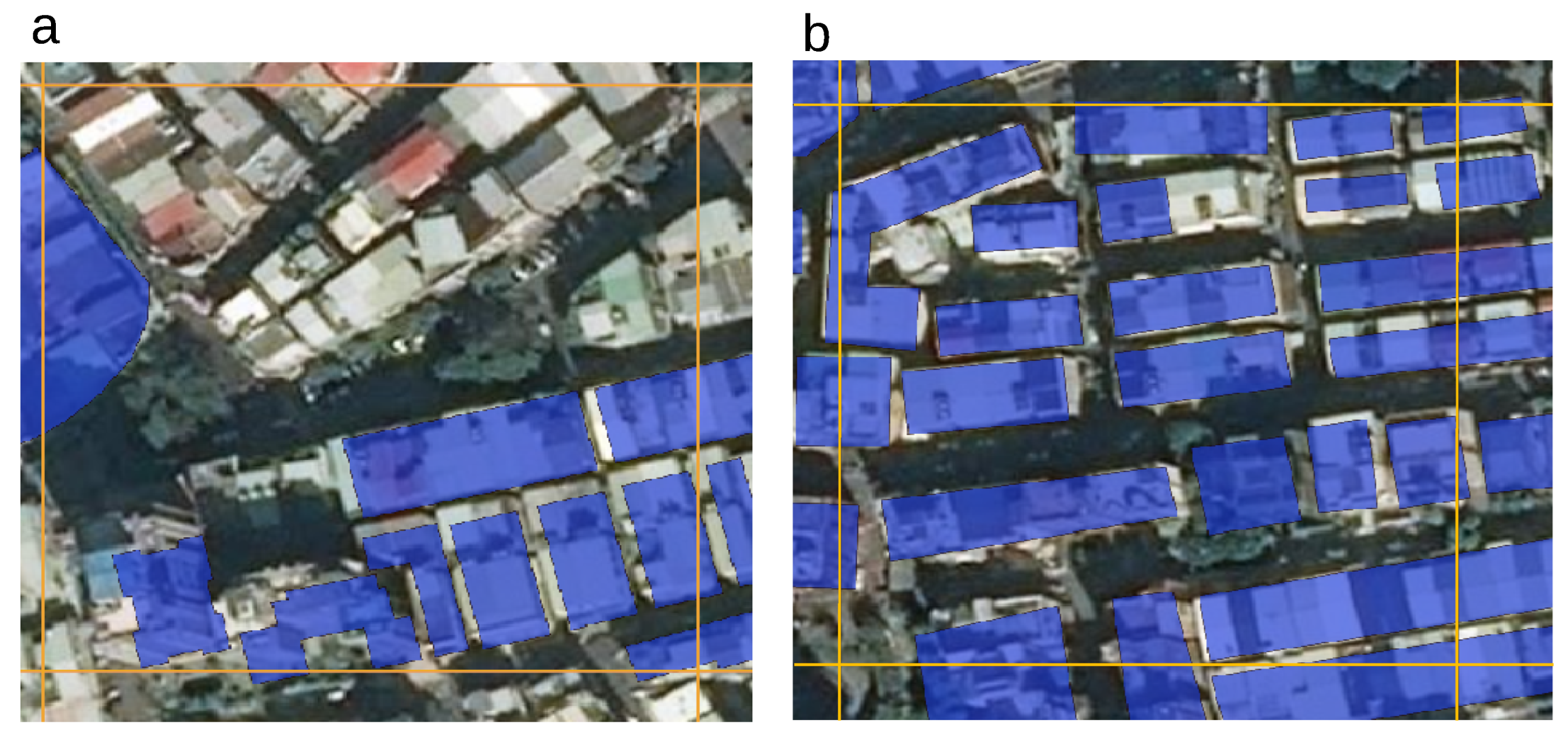
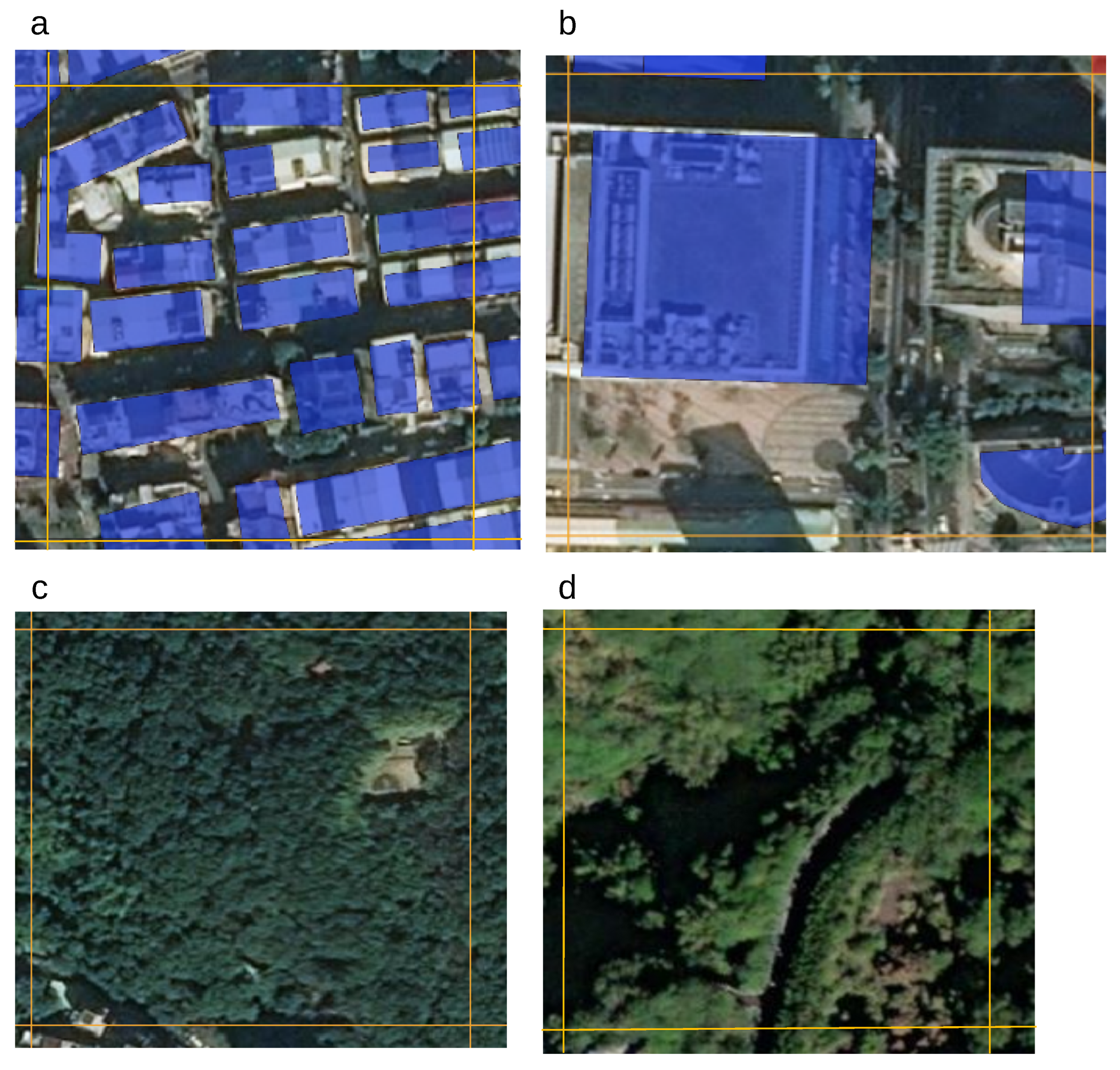
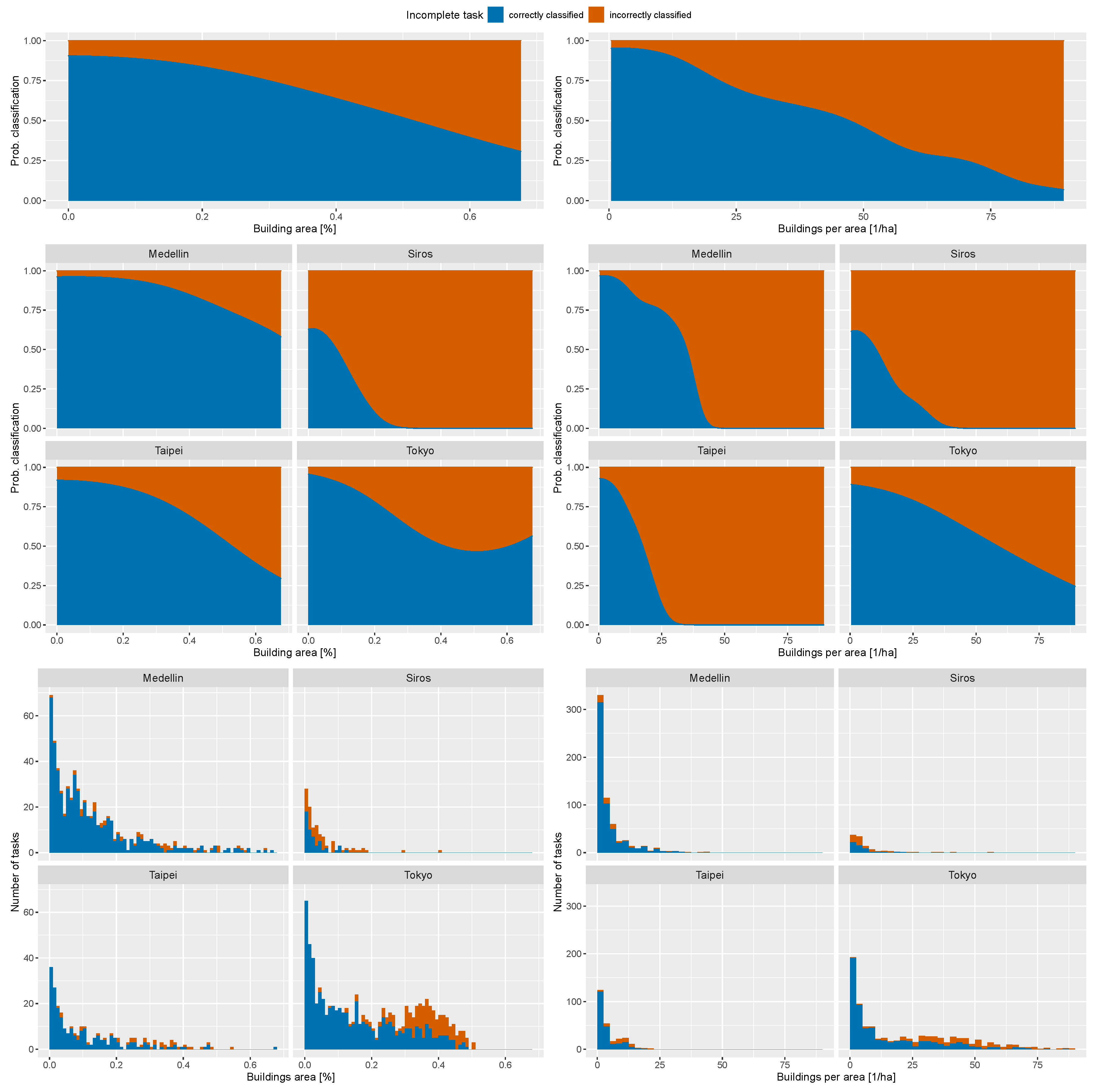
In this study, we analyzed the quality of the crowd-sourced classification of the completeness of OSM building footprints. We showed that the completeness feature in MapSwipe has the potential to produce spatially explicit information about the completeness of OSM building footprints. A factor that influenced the OSM building completeness classification were tasks with a high OSM building density, expressed both by the number of buildings or their footprint area. More buildings or a larger share of the area covered by building footprints distracted the users from a correct “incomplete” classification. After correcting for the correlated error structure, the share of the footprint area led to a slightly improved model compared to the model based on the number of buildings. Moreover, the classification performance was dependent on how exactly the OSM layer aligned with the satellite imagery. Presumably, the currentness of the satellite imagery used in MapSwipe is of importance for the quality of the assessment as well. Unfortunately, image offsets often differ between imagery from different providers. The offset might even vary across the imagery, especially in hilly or mountainous terrain. Using more recent imagery in MapSwipe than that used for the mapping of the buildings in OSM might therefore introduce a challenge for volunteers if this introduces an offset between OSM building footprints and imagery. Herfort et al. 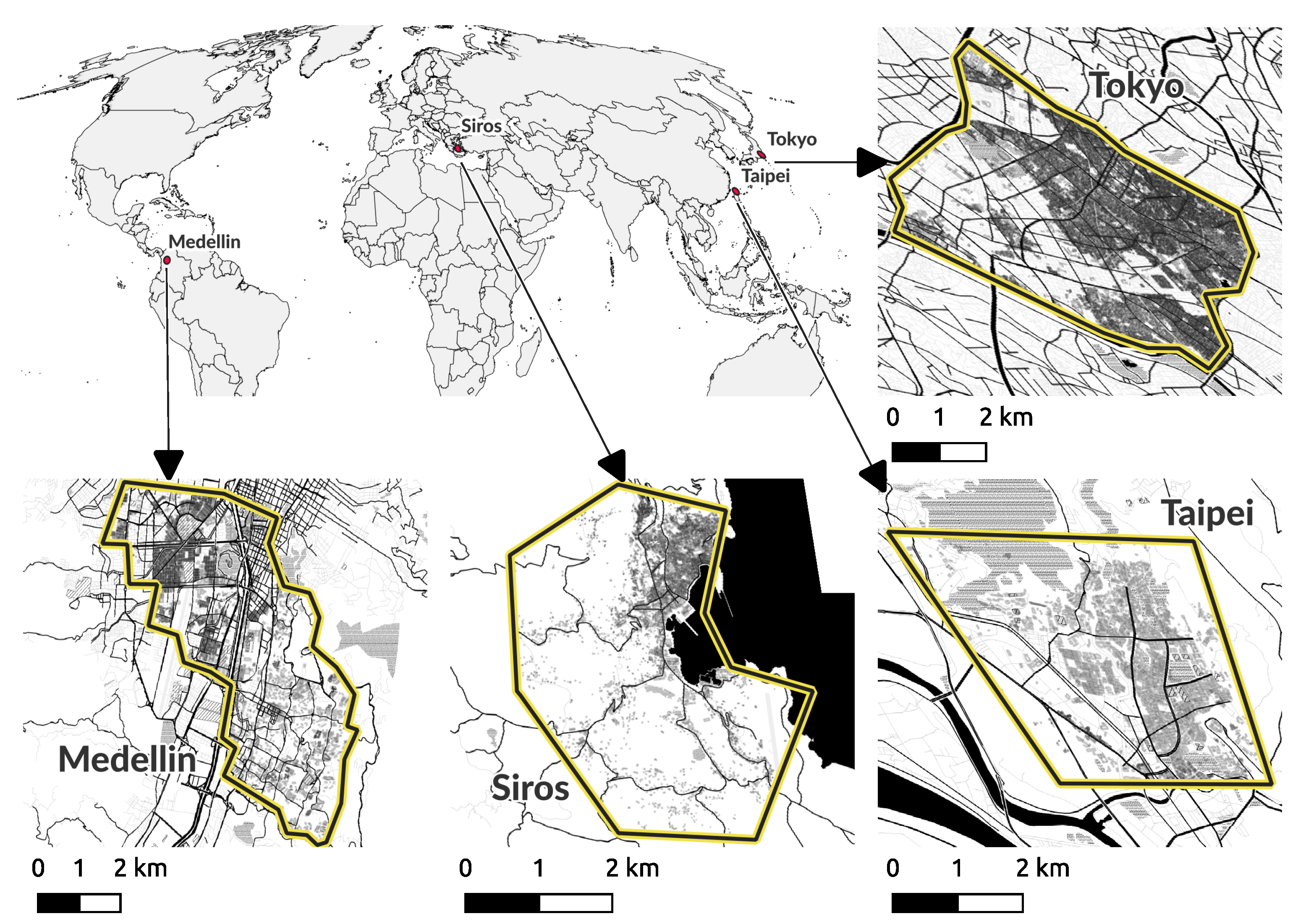[35] have shown that other factors, such as the resolution of the satellite imagery, missing images as well as presence of clouds, might also influence the quality of the classification. By successfully testing the approach at four different sites with different building textures, we suggest that the completeness feature in MapSwipe can be applied to most inhabited areas.

A main limitation of this study is the low number of volunteers taking part in the completeness mapping event. It is important to highlight that other authors have shown for OSM that a higher number of volunteers is positively related to the accuracy of the produced data [15]. Because the answer of each MapSwipe volunteer is also prone to errors, a larger group of volunteers would presumably reduce the overall uncertainty (“wisdom of the crowd”). The same applies to the number of experts. The quality of the classification task clearly depends not only on the properties of the task (such as building density, alignment of OSM and satellite imagery) but also on the experience of the volunteers with such pattern recognition tasks, on the knowledge of potential building types in the area as well as on factors influencing the concentration and motivation of the volunteers [55,56,57]. These factors are, by design, not available for the researcher as MapSwipe does not request personal data from the user.

A further limitation of this study was that incomplete tasks did not provide quantitative information about the number of missing buildings. Therefore, the completeness feature does not provide information about the share of missing buildings in the incomplete tasks. While it would be possible to extend the MapSwipe completeness tool with respect to additional classes—such as “mostly complete”, “up to 50% complete”, etc.—this would come at the cost of increasing complexity. MapSwipe was designed as a tool that requires only minimum training effort and that uses a simple and easy-to-learn user interface. Extending the tool with more complex features might reduce its attractiveness for its intended users. Future work will assess how far increasing the complexity of MapSwipe tasks correlates with decreasing user satisfaction and decreasing classification quality. The current idea is that MapSwipe is used to identify areas that demand more mapping and that the mapping itself is done in established OSM editors. The amount of missing buildings could later on be derived by an analysis of the newly mapped features by tools such as the ohsome API [23].

Herfort et al. [58] proposed a workflow combining deep-learning and crowd-sourcing methods to generate human settlement maps. An extension to this study could be used to perform an automated approach within the incomplete tiles in order to automatically identify the share of missing human settlements. Completely mapped tiles from nearby areas might be used in this context as a training dataset. As Pisl et al. [59] have shown, it is possible to fine-tune pre-trained deep neural networks for building detection based on a relatively small set of additional training data. Furthermore, new products such as the World Settlement Footprint 2015 or similar datasets on the global distribution of built-up areas have already relied on crowd-sourcing approaches to assess classification performance and completeness of built-up areas [60]. In this light, the completeness feature in MapSwipe could be used in future applications to complement automated approaches by generating training as well as validation datasets and could also address specific cases in which automated approaches do not perform well.

Despite the low number of volunteers taking part in the completeness mapping project, this study has shown the characteristics of the data produced by the completeness feature from MapSwipe, which can be useful for exposure models. The misclassifications mostly happened in nearly complete tasks. For exposure modeling, these are of minor importance, since results will only be affected marginally if a few buildings in nearly complete tiles are unmapped. It would have been more problematic if actually incomplete tiles with a big share of unmapped buildings had been considered as “complete”.

The comparison of the MapSwipe completeness assessment with the other two approaches showed clear differences. The comparison was complicated by the different spatial units as well as by the different granularity of the results, as the MapSwipe assessment returned only binary classification at the level of the tiles, while the comparison of model predictions with observed OSM buildings returned continuous complete estimates. For regions where only a few buildings are missing per tile, the MapSwipe-based assessment might therefore be too pessimistic. The quality of the intrinsic approach relies on a area what is big enough to capture the mapping dynamics in the region. The 2 km buffer chosen here might not be well suited for all study sites; further research is needed to establish better knowledge on adequate region sizes. The quality of the machine-learning-based approach [13] differs between urban areas, so it is not clear how well the model predicts the building footprints for a specific area. The MapSwipe assessment by volunteers was able to provide, for all three considered study sites, a good estimate for the expert judgment. The other two approaches showed stronger variability, which makes a judgment based on those approaches more uncertain for a new study site. In addition, one should consider that the volunteer-based approach offered a much finer and detailed view on the OSM completeness as it is available at the level of the MapSwipe tiles. The OSM completeness estimation based on the model by Herfort et al. [13] was currently only available for urban centers at 1 sqkm grid cell level, which might be sufficient enough for disaster-based applications. The intrinsic approach requires integration across larger areas and can therefore be less detailed. However, the different approaches presumably complement each other as the labor-intensive MapSwipe approach can only be applied to smaller-scale areas while the approach by Herfort et al. [13] provides coarser-scale prediction for urban centers worldwide and the intrinsic approach can be easily applied at a bit larger scale. The MapSwipe approach and the intrinsic approach can be extended to other OSM feature classes such as roads relatively easily, while the machine learning approach requires extensive training data as well as huge training effort for other OSM feature classes.

User experience presumably constitutes another relevant factor for the quality of contributions. As the new feature was tested in a developer instance of the app, it was, for the case study, not possible to quantify this effect. However, future work will investigate the effects of user experience on the classification performance of the users. This might lead to a new aggregation scheme across users, which may use MapSwipe experience as weights.

Further analysis should test extended possibilities for gamification of MapSwipe and how this affects user motivation. This might involve possibilities for the comparison of different users or rankings of users. We have provided such rankings on demand for a few organizations involved in larger MapSwipe campaigns. However, we were also confronted with the potential drawbacks of such rankings: these might stimulate low-quality classifications to speed up the swiping and to position one higher in the ranking.

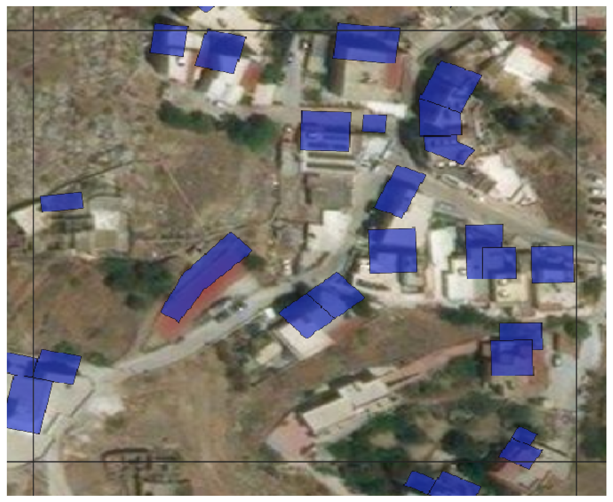
Another aspect that requires further improvement is the user interface. The way that OSM buildings are displayed in the tiles is currently optimized for OSM building visibility. The cost is that the semi-transparent filled polygons tend to hide the underlying parts of the satellite imagery. Extensive testing with users will be needed to identify a compromise that allows both to see the satellite imagery and to easily grasp the existing building footprints. As MapSwipe is used in very different geographic settings, a solution needs to work for different terrain and land-cover settings. In densely populated urban areas, images with a higher resolution than that of zoom level 18 could be beneficial. However, this requires the availability of drone or aerial imagery, which is, so far, only available for selected areas.

In our study, we focused on the completeness of buildings. An interesting application might be a local assessment of machine learning predictions such as the Microsoft buildings footprint [19]. The approach could, in principle, be extended also to other machine-learning-based feature predictions such as the Map With AI roads dataset by Facebook [61]. We can think of many other OSM classes such as land-use features or streets where a similar completeness-task design could be developed. In the domain of land-use and land-cover, classification studies that underline the potential of crowd-sourcing approaches for better earth observation already exist [62,63]. Further studies are needed to fully comprehend which OSM classes perform well and which OSM classes are too complex. The use of MapSwipe to detect incompletely mapped regions at a small scale is limited to tasks that can be easily detected based on satellite imagery. It is not a silver bullet approach suitable for all types of OSM aspects, but it complements other approaches such as intrinsic and extrinsic data-quality assessments, incorporation of other Volunteered Geographic Information sources such as Twitter [64] and awareness-raising campaigns for mapathons [65].

7. Conclusions

Our results demonstrate that the completeness feature for MapSwipe provides a good opportunity for the fast assessment of OSM building completeness at smaller scales, as is often required in a disaster setting. Building density was shown to affect the complexity of the task and, thereby, the reliability of the assessment. However, the quality of the assessment also differed clearly between the individual users. This offers opportunity for further research with respect to how individual factors, such as user experience, influence the quality of the assessment. The aggregation of feedback by the different users provided reliable estimates of completeness for the selected task. The tool complements other approaches to estimate OSM feature completeness in a region. It allowed to identify parts of an affected region that require more mapping of buildings at high spatial resolution. Intrinsic approaches, in contrast, require larger regions for reliable assessments as they work by integrating mapping history over time and space. If predictions by models such as the one used here are available, they might offer a good alternative as well. However, as long as these are not available for a required feature class, a combination of regional-scale assessment of intrinsic approaches and detailed evaluation by volunteers using the tool presented here can combine the best of both worlds to quickly assess data quality, which is often necessary in disaster contexts. For building footprints, a combination of all three presented approaches might be a suitable solution to obtain a timely estimation about where additional mapping effort is needed.

References

1. McGlade, J.; Bankoff, G.; Abrahams, J.; Cooper-Knock, S.; Cotecchia, F.; Desanker, P.; Erian, W.; Gencer, E.; Gibson, L.; Girgin, S.; et al. Global Assessment Report on Disaster Risk Reduction; United Nations Office for Disaster Risk Reduction: Geneva, Switzerland, 2019. [Google Scholar]
2. Birkmann, J. Measuring Vulnerability to Natural Hazards: Towards Disaster Resilient Societies, 2nd ed.; United Nations Univ. Press: Tokyo, Japan, 2013. [Google Scholar]
3. Pittore, M.; Wieland, M.; Fleming, K. Perspectives on global dynamic exposure modelling for geo-risk assessment. Nat. Hazards 2017, 86, 7–30. [Google Scholar] [CrossRef]
4. Shan, S.; Zhao, F.; Wei, Y.; Liu, M. Disaster management 2.0: A real-time disaster damage assessment model based on mobile social media data—A case study of Weibo (Chinese Twitter). Saf. Sci. 2019, 115, 393–413. [Google Scholar] [CrossRef]
5. Peduzzi, P.; Dao, H.; Herold, C.; Mouton, F. Assessing global exposure and vulnerability towards natural hazards: The Disaster Risk Index. Nat. Hazards Earth Syst. Sci. 2009, 9, 1149–1159. [Google Scholar] [CrossRef]
6. De Bono, A.; Mora, M.G. A global exposure model for disaster risk assessment. Int. J. Disaster Risk Reduct. 2014, 10, 442–451. [Google Scholar] [CrossRef]
7. Gunasekera, R.; Ishizawa, O.; Aubrecht, C.; Blankespoor, B.; Murray, S.; Pomonis, A.; Daniell, J. Developing an adaptive global exposure model to support the generation of country disaster risk profiles. Earth-Sci. Rev. 2015, 150, 594–608. [Google Scholar] [CrossRef] [Green Version]
8. Poiani, T.H.; Dos Santos Rocha, R.; Degrossi, L.C.; Porto De Albuquerque, J. Potential of Collaborative Mapping for Disaster Relief: A Case Study of OpenStreetMap in the Nepal Earthquake 2015. In Proceedings of the 2016 49th Hawaii International Conference on System Sciences (HICSS), Koloa, HI, USA, 5–8 January 2016; pp. 188–197. [Google Scholar] [CrossRef]
9. Goldblatt, R.; Jones, N.; Mannix, J. Assessing OpenStreetMap Completeness for Management of Natural Disaster by Means of Remote Sensing: A Case Study of Three Small Island States (Haiti, Dominica and St. Lucia). Remote Sens. 2020, 12, 118. [Google Scholar] [CrossRef] [Green Version]
10. Hecht, R.; Kunze, C.; Hahmann, S. Measuring Completeness of Building Footprints in OpenStreetMap over Space and Time. ISPRS Int. J. Geo-Inf. 2013, 2, 1066–1091. [Google Scholar] [CrossRef]
11. Herfort, B.; Lautenbach, S.; Porto de Albuquerque, J.; Anderson, J.; Zipf, A. The evolution of humanitarian mapping within the OpenStreetMap community. Sci. Rep. 2021, 11, 3037. [Google Scholar] [CrossRef]
12. Brückner, J.; Schott, M.; Zipf, A.; Lautenbach, S. Assessing shop completeness in OpenStreetMap for two federal states in Germany. AGILE GIScience Ser. 2021, 2, 1–7. [Google Scholar] [CrossRef]
13. Herfort, B.; Lautenbach, S.; de Albuquerque, J.P.; Anderson, J.; Zipf, A. Investigating the digital divide in OpenStreetMap: Spatio-temporal analysis of inequalities in global urban building completeness. 2022. preprint. [Google Scholar] [CrossRef]
14. Quattrone, G.; Mashhadi, A.; Capra, L. Mind the map: The impact of culture and economic affluence on crowd-mapping behaviours. In Proceedings of the 17th ACM Conference on Computer Supported Cooperative Work & Social Computing-CSCW’14, Baltimore, MD, USA, 15–19 February 2014; ACM Press: Baltimore, MD, USA, 2014; pp. 934–944. [Google Scholar] [CrossRef]
15. Haklay, M.; Basiouka, S.; Antoniou, V.; Ather, A. How Many Volunteers Does it Take to Map an Area Well? The Validity of Linus’ Law to Volunteered Geographic Information. Cartogr. J. 2010, 47, 315–322. [Google Scholar] [CrossRef] [Green Version]
16. Törnros, T.; Dorn, H.; Hahmann, S.; Zipf, A. Uncertainties of completeness measures in OpenStreetMap–A case study for buildings in a medium-sized German city. ISPRS Ann. Photogramm. Remote Sens. Spat. Inf. Sci. 2015, 2, 353. [Google Scholar] [CrossRef] [Green Version]
17. Biljecki, F.; Chew, L.Z.X.; Milojevic-Dupont, N.; Creutzig, F. Open government geospatial data on buildings for planning sustainable and resilient cities. arXiv 2021, arXiv:2107.04023. [Google Scholar]
18. Schott, M.; Zell, A.; Lautenbach, S.; Demir, B.; Zipf, A. Returning the Favor—Leveraging Quality Insights of OpenStreetMap-Based Land-Use/Land-Cover Multi-Label Modeling to the Community. In Proceedings of the Academic Track at State of the Map 2022, Florence, Italy, 19–21 August 2022. [Google Scholar] [CrossRef]
19. Microsoft. Microsoft Building Footprints. 2022. Available online: https://github.com/microsoft/GlobalMLBuildingFootprints (accessed on 9 March 2023).
20. Zielstra, D.; Zipf, A. Quantitative Studies on the Data Quality of OpenStreetMap in Germany. GIScience 2010, 2010, 8. [Google Scholar]
21. Barron, C.; Neis, P.; Zipf, A. A Comprehensive Framework for Intrinsic OpenStreetMap Quality Analysis. Trans. GIS 2014, 18, 877–895. [Google Scholar] [CrossRef]
22. Minghini, M.; Brovelli, M.A.; Frassinelli, F. An Open Source Approach for the Intrinsic Assessment of the Temporal Accuracy, Up-to-dateness and lineage of OpenStreetMap. ISPRS—Int. Arch. Photogramm. Remote Sens. Spat. Inf. Sci. 2018, XLII-4/W8, 147–154. [Google Scholar] [CrossRef] [Green Version]
23. Raifer, M.; Troilo, R.; Kowatsch, F.; Auer, M.; Loos, L.; Marx, S.; Przybill, K.; Fendrich, S.; Mocnik, F.B.; Zipf, A. OSHDB: A framework for spatio-temporal analysis of OpenStreetMap history data. Open Geospat. Data, Softw. Stand. 2019, 4, 3. [Google Scholar] [CrossRef] [Green Version]
24. Senaratne, H.; Mobasheri, A.; Ali, A.L.; Capineri, C.; Haklay, M.M. A review of volunteered geographic information quality assessment methods. Int. J. Geogr. Inf. Sci. 2017, 31, 139–167. [Google Scholar] [CrossRef] [Green Version]
25. Gröchenig, S.; Brunauer, R.; Rehrl, K. Estimating Completeness of VGI Datasets by Analyzing Community Activity Over Time Periods. In Connecting a Digital Europe Through Location and Place; Huerta, J., Schade, S., Granell, C., Eds.; Lecture Notes in Geoinformation and Cartography; Springer International Publishing: Cham, Switzerland, 2014; pp. 3–18. [Google Scholar] [CrossRef]
26. Yeboah, G.; Porto de Albuquerque, J.; Troilo, R.; Tregonning, G.; Perera, S.; Ahmed, S.A.K.S.; Ajisola, M.; Alam, O.; Aujla, N.; Azam, S.I.; et al. Analysis of OpenStreetMap Data Quality at Different Stages of a Participatory Mapping Process: Evidence from Slums in Africa and Asia. ISPRS Int. J. Geo-Inf. 2021, 10, 265. [Google Scholar] [CrossRef]
27. Zhou, Q. Exploring the relationship between density and completeness of urban building data in OpenStreetMap for quality estimation. Int. J. Geogr. Inf. Sci. 2018, 32, 257–281. [Google Scholar] [CrossRef]
28. Zhou, Q.; Tian, Y. The use of geometric indicators to estimate the quantitative completeness of street blocks in OpenStreetMap. Trans. GIS 2018, 22, 1550–1572. [Google Scholar] [CrossRef]
29. Camboim, S.; Bravo, J.; Sluter, C. An Investigation into the Completeness of, and the Updates to, OpenStreetMap Data in a Heterogeneous Area in Brazil. ISPRS Int. J. Geo-Inf. 2015, 4, 1366–1388. [Google Scholar] [CrossRef] [Green Version]
30. Neis, P.; Zielstra, D.; Zipf, A. Comparison of volunteered geographic information data contributions and community development for selected world regions. Future Internet 2013, 5, 282–300. [Google Scholar] [CrossRef] [Green Version]
31. Schott, M.; Lautenbach, S.; Größchen, L.; Zipf, A. OpenStreetMap Element Vectorisation—A tool for high resolution data insights and its usability in the land-use and land-cover domain. Int. Arch. Photogramm. Remote Sens. Spat. Inf. Sci. 2022, XLVIII-4/W1-2022, 395–402. [Google Scholar] [CrossRef]
32. HOT. The Humanitarian OpenStreetMap Team. 2023. Available online: https://www.hotosm.org/ (accessed on 9 March 2023).
33. Missing Maps Network. Putting the World’s Vulnerable Communities on the Map. 2023. Available online: https://www.missingmaps.org/ (accessed on 9 March 2023).
34. MapSwipe Developers. MapSwipe. 2023. Available online: https://mapswipe.org/ (accessed on 9 March 2023).
35. Herfort, B.; Reinmuth, M.; De Albuquerque, J.P.; Zipf, A. Towards evaluating crowdsourced image classification on mobile devices to generate geographic information about human settlements. In Proceedings of the Societal Geo-Innovation: Short Papers, Posters and Poster Abstracts of the 20th AGILE Conference on Geographic Information Science, Wageningen, The Netherlands, 9–12 May 2017; Bregt, A., Sarjakoski, T., Lammeren, R., van Rip, F., Eds.; Wageningen University & Research: Wageningen, Netherlands, 2017. [Google Scholar]
36. MapSwipe Developers. MapSwipe Data. 2023. Available online: https://mapswipe.org/en/data.html (accessed on 9 March 2023).
37. Scholz, S.; Knight, P.; Eckle, M.; Marx, S.; Zipf, A. Volunteered Geographic Information for Disaster Risk Reduction: The Missing Maps Approach and Its Potential within the Red Cross and Red Crescent Movement. Remote Sens. 2018, 10, 1239. [Google Scholar] [CrossRef] [Green Version]
38. Baruch, A.; May, A.; Yu, D. The motivations, enablers and barriers for voluntary participation in an online crowdsourcing platform. Comput. Hum. Behav. 2016, 64, 923–931. [Google Scholar] [CrossRef] [Green Version]
39. Morschheuser, B.; Hamari, J.; Koivisto, J.; Maedche, A. Gamified crowdsourcing: Conceptualization, literature review, and future agenda. Int. J. Hum.-Comput. Stud. 2017, 106, 26–43. [Google Scholar] [CrossRef] [Green Version]
40. Neis, P. How Did You Contribute to OSM? 2023. Available online: http://hdyc.neis-one.org/ (accessed on 9 March 2023).
41. Neis, P. OSM Fight. 2023. Available online: http://osmfight.neis-one.org/ (accessed on 9 March 2023).
42. Kohns, J.; Zahs, V.; Ullah, T.; Schorlemmer, D.; Nievas, C.; Glock, K.; Meyer, F.; Mey, H.; Stempniewski, L.; Herfort, B.; et al. Innovative methods for earthquake damage detection and classification using airborne observation of critical infrastructures (project LOKI), 2021. In Proceedings of the EGU 2021 Proceedings, EGU General Assembly 2021, Online. 19–30 April 2021. [Google Scholar] [CrossRef]
43. MapSwipe Developers. MapSwipeDev-API. 2023. Available online: https://dev.mapswipe.org/api/agg_results/ (accessed on 9 March 2023).
44. Albuquerque, J.; Herfort, B.; Eckle, M. The Tasks of the Crowd: A Typology of Tasks in Geographic Information Crowdsourcing and a Case Study in Humanitarian Mapping. Remote Sens. 2016, 8, 859. [Google Scholar] [CrossRef] [Green Version]
45. R Core Team. R: A Language and Environment for Statistical Computing; R Foundation for Statistical Computing: Vienna, Austria, 2021. [Google Scholar]
46. Pebesma, E. Simple Features for R: Standardized Support for Spatial Vector Data. R J. 2018, 10, 439. [Google Scholar] [CrossRef] [Green Version]
47. Wickham, H.; Averick, M.; Bryan, J.; Chang, W.; McGowan, L.D.; François, R.; Grolemund, G.; Hayes, A.; Henry, L.; Hester, J.; et al. Welcome to the tidyverse. J. Open Source Softw. 2019, 4, 1686. [Google Scholar] [CrossRef] [Green Version]
48. Pebesma, E. lwgeom: Bindings to Selected ’liblwgeom’ Functions for Simple Features. 2020. Available online: https://CRAN.R-project.org/package=lwgeom (accessed on 25 March 2020).
49. Bolker, B.M.; Brooks, M.E.; Clark, C.J.; Geange, S.W.; Poulsen, J.R.; Stevens, M.H.H.; White, J.S.S. Generalized linear mixed models: A practical guide for ecology and evolution. Trends Ecol. Evol. 2009, 24, 127–135. [Google Scholar] [CrossRef]
50. Schielzeth, H.; Nakagawa, S. Nested by design: Model fitting and interpretation in a mixed model era. Methods Ecol. Evol. 2013, 4, 14–24. [Google Scholar] [CrossRef]
51. Zuur, A.F.; Ieno, E.; Walker, N.J.; Saveliev, A.A.; Smithe, G.M. Mixed Effect Models and Extensions in Ecology with R; Springer: Berlin/Heidelberg, Germany, 2009. [Google Scholar] [CrossRef]
52. Bates, D.; Mächler, M.; Bolker, B.; Walker, S. Fitting Linear Mixed-Effects Models Using lme4. J. Stat. Softw. 2015, 67, 1–48. [Google Scholar] [CrossRef]
53. Nakagawa, S.; Schielzeth, H. A general and simple method for obtaining R 2 from generalized linear mixed-effects models. Methods Ecol. Evol. 2013, 2, 133–142. [Google Scholar] [CrossRef]
54. Fritz, O. ohsome: An ‘ohsome API’ Client. 2023. Available online: https://cran.r-project.org/web/packages/ohsome/ (accessed on 15 March 2023).
55. Antoniou, V.; Skopeliti, A. Measures and indicators of VGAI: An overview. ISPRS Ann. Photogramm. Remote. Sens. Spat. Inf. Sci. 2015, II-3/W5, 345–351. [Google Scholar] [CrossRef] [Green Version]
56. Comber, A.; Mooney, P.; Purves, R.S.; Rocchini, D.; Walz, A. Crowdsourcing: It Matters Who the Crowd Are. The Impacts of between Group Variations in Recording Land Cover. PLoS ONE 2016, 11, e0158329. [Google Scholar] [CrossRef] [Green Version]
57. Eckle, M.; de Albuquerque, J.P. Quality Assessment of Remote Mapping in OpenStreetMap for Disaster Management Purposes. In Proceedings of the Geospatial Data and Geographical Information Science Proceedings of the ISCRAM 2015 Conference, Krystiansand, Norway, 24–27 May 2015. [Google Scholar]
58. Herfort, B.; Li, H.; Fendrich, S.; Lautenbach, S.; Zipf, A. Mapping Human Settlements with Higher Accuracy and Less Volunteer Efforts by Combining Crowdsourcing and Deep Learning. Remote Sens. 2019, 11, 1799. [Google Scholar] [CrossRef] [Green Version]
59. Pisl, J.; Li, H.; Lautenbach, S.; Herfort, B.; Zipf, A. Detecting OpenStreetMap missing buildings by transferring pre-trained deep neural networks. AGILE: GIScience Ser. 2021, 2, 1–7. [Google Scholar] [CrossRef]
60. Marconcini, M.; Metz-Marconcini, A.; Üreyen, S.; Palacios-Lopez, D.; Hanke, W.; Bachofer, F.; Zeidler, J.; Esch, T.; Gorelick, N.; Kakarla, A.; et al. Outlining where humans live, the World Settlement Footprint 2015. Sci. Data 2020, 7, 242. [Google Scholar] [CrossRef] [PubMed]
61. Facebook. Open Mapping At Facebook. 2023. Available online: https://github.com/facebookmicrosites/Open-Mapping-At-Facebook (accessed on 9 March 2023).
62. Fonte, C.; Minghini, M.; Patriarca, J.; Antoniou, V.; See, L.; Skopeliti, A. Generating Up-to-Date and Detailed Land Use and Land Cover Maps Using OpenStreetMap and GlobeLand30. ISPRS Int. J. Geo-Inf. 2017, 6, 125. [Google Scholar] [CrossRef] [Green Version]
63. Vargas-Munoz, J.E.; Srivastava, S.; Tuia, D.; Falcão, A.X. OpenStreetMap: Challenges and Opportunities in Machine Learning and Remote Sensing. IEEE Geosci. Remote Sens. Mag. 2021, 9, 184–199. [Google Scholar] [CrossRef]
64. Li, H.; Herfort, B.; Huang, W.; Zia, M.; Zipf, A. Exploration of OpenStreetMap missing built-up areas using twitter hierarchical clustering and deep learning in Mozambique. ISPRS J. Photogramm. Remote Sens. 2020, 166, 41–51. [Google Scholar] [CrossRef]
65. Mobasheri, A.; Zipf, A.; Francis, L. OpenStreetMap data quality enrichment through awareness raising and collective action tools—experiences from a European project. Geo-Spat. Inf. Sci. 2018, 21, 234–246. [Google Scholar] [CrossRef] [Green Version]
Figure 1. MapSwipe main screen. Two examples are given: (a) Green-colored tiles represent complete tiles, untapped tiles represent no building tiles; (b) Orange-colored tiles represent areas that are incompletely mapped in OSM with respect to building footprints.
Ijgi 12 00143 g001
Figure 2. Case study locations. The completeness of mapping in OSM differed across and within the case studies. However, all four case studies contained a large number of OSM features as indicated by the detail maps which were limited for this figure to the most relevant features (main roads and building footprints). Data source: OpenStreetMap contributors under ODbL and Natural Earth (world map). Map tiles for detailed maps by Carto, under CC BY 3.0.
Ijgi 12 00143 g002
Figure 3. (a) Example of a task with low OSM building completeness; (b) example of a task with almost complete OSM building coverage.
Ijgi 12 00143 g003
Figure 4. Examples for mismatches between volunteer and expert assessment: (a) Tasks predicted as complete, true class is incomplete; (b) Tasks predicted as incomplete, true class is complete; (c) Tasks predicted as no building, true class is incomplete; (d) Tasks predicted as incomplete, true class is no building. Shown are MapSwipe tiles with the OSM building footprints (blue) overlaid.
Ijgi 12 00143 g004
Figure 5. Example for a misalignment of the OSM building footprint layer and satellite imagery. The example is taken from the case study at Sirios.
Ijgi 12 00143 g005
Figure 6. Conditional density plots for the classification correctness of tasks classified as “incomplete” by the volunteers dependent on the part of the task area covered by buildings (left column) or the number of buildings per hectare (right column). In addition to the plots for all sites (first row), site-specific conditional density plots are shown (second row) as well as the distribution of the explanatory variable through histograms (last row). The histograms show the two classes in a stacked way.
Ijgi 12 00143 g006