A Contour Line Group Simplification Method Based on Classified Terrain Features

Abstract

Contour line group simplification methods can effectively preserve terrain features during map making and producing. This process involves two main steps, namely terrain feature line extraction and contour bend selection. The terrain feature line extraction includes two steps, that is, terrain feature point extraction and classification, and terrain feature line connection. However, to date, many similar studies have not considered the hierarchy of terrain features. Therefore, we proposed a group simplification method for contour lines based on classified terrain features and tested it on a study area with mainly positive landforms. In accordance with geomorphological theory, we divided valleys into either gradually descending or ordinary. Valley points were extracted based on the constrained Delaunay triangulation method and then classified into the two categories. Gradually descending and ordinary valley lines were then connected. The contour bends were grouped based on the valley lines extracted and then selected according to the geometric indicators of the bend group. The results have demonstrated that the valley lines extracted closely matched human perception in integrity and structure. Contour lines simplified by our method achieved effective reduction of map information and adequate retention of the main terrain structures, which are similar to those from manual simplification.

1. Introduction

Contour lines can be used to represent the surface relief of the earth in a two-dimensional way, which is an essential element of topographic maps [1]. Due to the large volume of the contour line data, processing it during manual cartographic generalization is time consuming. Therefore, using an automated contour line simplification algorithm can substantially improve the efficiency of map making and producing.

Line simplification is one of the key research areas in the field of automated cartographic generalization [2]. Classic methods, such as the Douglas–Peucker [3], Li–Openshaw [4], and Visvalingam–Whyatt [5] algorithms have been applied successfully in simplifying real-world elements such as rivers and roads. Contours simulate three-dimensional (3D) terrain and their structural features need to be preserved during the simplification process. However, the classic algorithms are not well-suited to contour lines in this respect. In the context of contour line simplification, researchers have achieved impressive results in areas such as single-line simplification [6,7,8,9,10,11], group simplification [12,13,14,15], and 3D simplification algorithms [16,17,18].

Single-line simplification algorithms simplify each contour line separately and can be used to select points or bends from the perspective of graphics. Tutić et al. [6] proposed a method for simplifying contour lines with the distinct feature of area preservation. Qian et al. [7] suggested a new line simplification approach that maintains the general curve characteristics based on using the Oblique-Dividing-Curve method to identify U- and V-shaped contour curves. Zhu et al. [8] presented a method for identifying and structuring contour valley bends that achieves simplification through bend selection. According to Mozas-Calvache et al. and Gokgoz [9,10], an error band could be applied to contour line simplification that effectively avoids intersections while ensuring accuracy. On this basis, He et al. [11] proposed a new simplification method based on the two-level Bellman–Ford algorithm. Single-line simplification algorithms exclude the relationship between adjacent contour lines, which means that they cannot effectively maintain the main terrain features.

Group simplification algorithms first identify the overall groups of bends of ridges or valleys and then undertake simplification by retaining or deleting these ridges or valleys. Zheng et al. [12] proposed using a contour tree to improve contour line generalization. Ai [13] used the Delaunay triangulation network (DTN) model to detect valley feature points of contour lines and connect them to form a valley network and achieved contour line group simplification. Yang and Liu [14] suggested a method for evaluating the importance of terrain feature points and feature lines for selecting contour bends. Lan et al. [15] used the length and level of terrain feature lines to select contour bends. However, existing group simplification algorithms have not given adequate consideration to the hierarchy of terrain features.

The 3D simplification algorithms convert contour points into discrete points in 3D space and achieve simplification based on the selection of these points [16]. Dou and Zhang [17] improved the efficiency of the algorithm for processing large volumes of data by enhancing the method for determining the origin, anchor point, and initial floating point of the base plane. Cheng et al. [18] extended this method for integrated simplification of contour lines and rivers. When sorting discrete points, the weights of points located on rivers are higher than those of the points on contour lines to prevent inconsistencies between elements after generalization. Breaking contour lines into discrete points destroys the continuity of contour lines and leads to dissimilarity of adjacent contour bends, which is disadvantageous to terrain feature representation.

Among these three algorithm types, group simplification algorithms process contour lines based on terrain structures, which are closest to the traditional manual generalization method and can better maintain natural geographic features. The land surface can be divided into positive landforms and negative landforms. Positive landforms refer to surfaces with elevations that are higher than those of the surrounding area, such as mountain peaks and ridges. Conversely, negative landforms are concave terrain forms, such as basins and valleys. When mapping areas dominated by positive landforms, the aim of contour line generalization is to reduce the valleys and expand the ridges. In areas dominated by negative landforms, the aim is to expand the valleys and reduce the ridges.

The most important and challenging part of this method is identifying terrain structures. Relevant research has tended to use terrain feature lines to represent terrain structures, showing the geomorphology by depicting the directions of ridges and valleys [19]. Terrain feature line extraction can be divided into three steps, namely extraction of terrain feature points, identification of terrain feature point types, and connection of terrain feature lines. Terrain feature point extraction methods include the DTN method [19,20,21], the split method [22,23,24], and the multi-indicator method [25,26]. The DTN method uses contour points to establish a Delaunay triangulation network and determines the locations of terrain feature points based on the positional relationships between triangles. The principle behind the split method is the same as that of the Douglas–Peucker algorithm. This means that it involves searching for terrain features by recursively finding points with the largest distance. The multi-indicator method uses geometric indicators such as curvature, angle, and distance to establish a criterion for determining feature points. Once the terrain feature points have been determined, they are evaluated according to the elevation relationship on both sides of the contour line to distinguish between the ridge and valley points [27]. The connection between the terrain feature lines matches the feature points one by one, in order, based on factors such as the distance, angle, and topological relationship. The ridgelines are tracked along ascending contour lines, while the valley lines are tracked along descending contour lines. Nevertheless, the horizontal distance between adjacent contour bends may vary and there may be deep turns between bends. Therefore, using this method for a large-scale map could cause errors in the tracking of terrain feature lines or misrepresent the terrain structure of a region.

Cartography is becoming an increasingly interdisciplinary practice [28], and our study has applied relevant geomorphological knowledge to the cartographic generalization of contour lines. To overcome the shortcomings of existing methods, we proposed a valley classification method for contour line grouping based on the theory of surface morphology development in geomorphology. We used a predominantly positive landform area in the algorithm design, because most areas were dominated by positive landforms. Valley lines were extracted to group the valley bends for selection according to the contour line generalization principle. Our proposed method for simplifying the grouped contour lines was based on this.

The remainder of this paper is organized as follows. Section 2 introduces the background knowledge on surface morphology development in geomorphology and then distinguishes between gradually descending and ordinary valleys. Section 3 elaborates on the valley line extraction and classification method and the contour line simplification method through bend group selection. Section 4 describes the experimental design and data analysis. Section 5 summarizes the study conclusions and indicates future improvements of this study.

2. Background to the Study

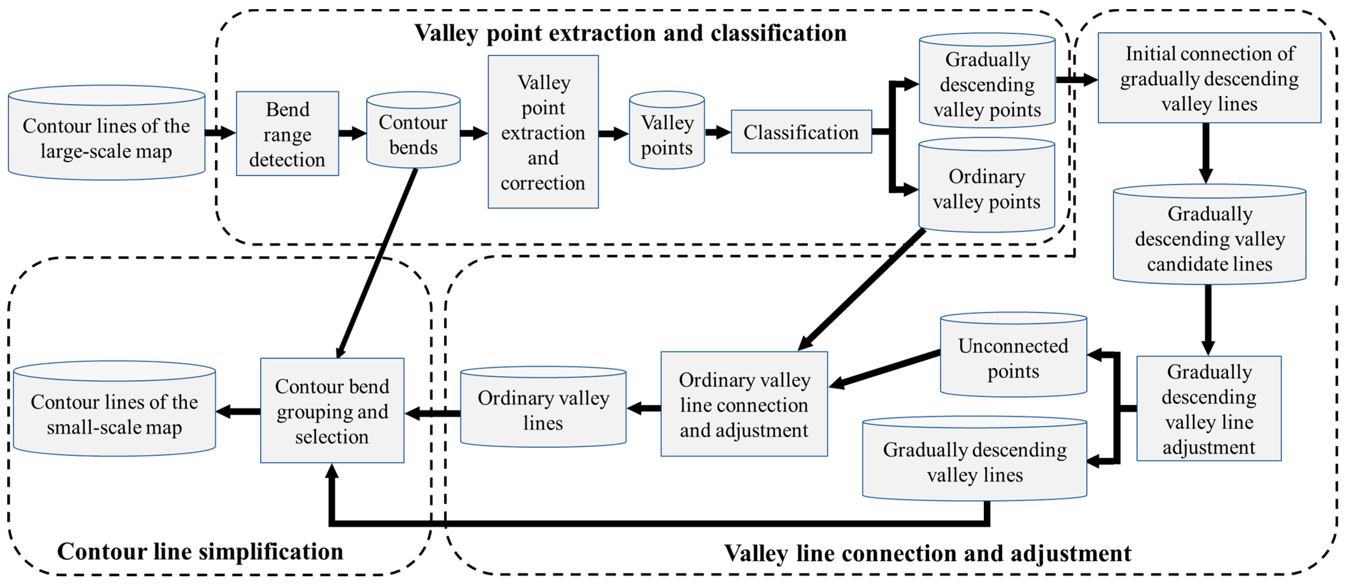
Water flow is one of the main external forces that can change the morphology of the land surface. As sheet-like water flows caused by rainfall on slopes are dispersed, low mechanical forces are generated, with a limited effect on the surface morphology. However, when sheet-like water flows move to lower terrains under the action of gravity, they form linear water flows that become increasingly concentrated. The mechanical force generated by linear water flows also increases, causing substantial land-surface erosion. The development of a valley from linear water erosion occurs in three stages, that is, valley incision, erosion, and depression [29]. During these processes, the valley floor is continuously eroded, and its height is gradually reduced at each stage. The lower the terrain, the greater the water flow, and the stronger the erosion, thereby changing the uniform slope of the original water confluence line, as shown by the brown curves in Figure 1. The original water confluence line is $H\to a\to b\to c\to L$, which changes to $H\to a\to b\to d\to L$, subsequently to $H\to a\to e\to L$, and, finally, to $H\to f\to L$. The downstream valley floor gradually descends, and valleys in previous stages of development converge to form a valley network. In this study, we divided valleys into gradually descending and ordinary valleys based on the characteristics of valley development.

In gradually descending valleys, the elevation of the valley floor gently changes in the direction of the valley extension. Such valleys are either well-developed eroded valleys or depressions. They are an integral part of a valley network that need to be preserved as major terrain structures during contour line generalization. The distances between adjacent contour lines, through gradually descending valleys, are relatively large. The connection of gradually descending valleys is easily affected by other valley points when traditional algorithms have been used to track terrain feature lines, which can result in connection errors.

Ordinary valleys refer to those that are not gradually descending. On a map, the distances between the adjacent contour lines of these valleys are relatively short and their topographic trends are relatively clear. Ordinary valleys include those with lower levels in the valley network. These valleys should be selected based on their geometric indicators during contour line generalization. An example of a gradually descending valley and ordinary valleys shown using 3-dimentional terrain modeling is shown in Figure 2.

Dividing valleys into these two categories for extraction has the following advantages. First, the resulting valley line connections closely match human perception. Extracting valley lines corresponding to gradually descending valleys reduces connection errors. The connections of valley lines corresponding to ordinary valleys can be controlled, making it relatively easy to connect valley lines into a tree structure. Reference information for contour line simplification has been provided. The importance of gradually descending valleys necessitates retention of the bends to prevent misrepresentation of crucial terrain features.

3. Methodology

The process used to extract and classify valley points, classify and connect valley lines, and select contour bend groups is shown in Figure 3. In Figure 3, cylinders show the status of the data, and boxes show the operation. There are three stages in our method, that is, valley point extraction and classification, valley line connection and adjustment, and contour line simplification. In the first stage, valley bends are detected, and then valley points of each bend are extracted and classified. In the second stage, valley lines are connected based on different types and adjusted. In the final stage, contour bends are grouped according to the valley lines obtained in the second stage, and the simplification of contour lines is accomplished by elimination of the valley bend groups.

3.1. Valley Point Extraction and Classification

Valley points are intersection points of a valley floor extension line and contour lines. Valley bends are contour line sections which convex to the uphill direction, and end points of valley bends are contour points at both ends. An example of valley bends, valley points, and end points of valley bends is shown in Figure 4. The extraction of valley points should balance two aspects, namely being placed at the center of the valley bend and maximizing the curvature and deviation. The terrain feature point extraction algorithm based on a constrained Delaunay triangulation network (DTN) [19] can be used to locate valley points almost at the center of the valley bends, thereby facilitating the connection of the valley lines. However, some points that are more suitable as valley points, with relatively large curvatures or deviations, could be discarded. Multiple valley points could be extracted at a valley bend near the intersection of multiple valleys, which could cause the same bend to be grouped multiple times during subsequent contour line simplification. In this study, we improved the algorithm to enable correction of problematic valley points based on point curvature. Furthermore, our method eliminates the shortcomings of the curvature-based extraction method that is sensitive to the distribution of points [21]. The process has been described as follows.

• We adjusted the order of contour points so that the left side of the forward direction of each contour point was the direction of elevation rise.
• The valley-side bends of each contour line were detected based on the vector cross product method [8]. For open contour lines, we calculated the cross product of the vectors obtained by connecting two adjacent points starting from the first point, with successive cross products below zero recorded as valley bends. For closed contour lines, if the vector cross products formed by the first point and the points on either side were not greater than zero, the point sequence was reversed to find the original point of the bend on which the first point was located. It was then necessary to search for the end point of the bend, starting with the first point, to obtain the point range of the first valley bend. The remainder of the process was the same as that used for open contour lines.
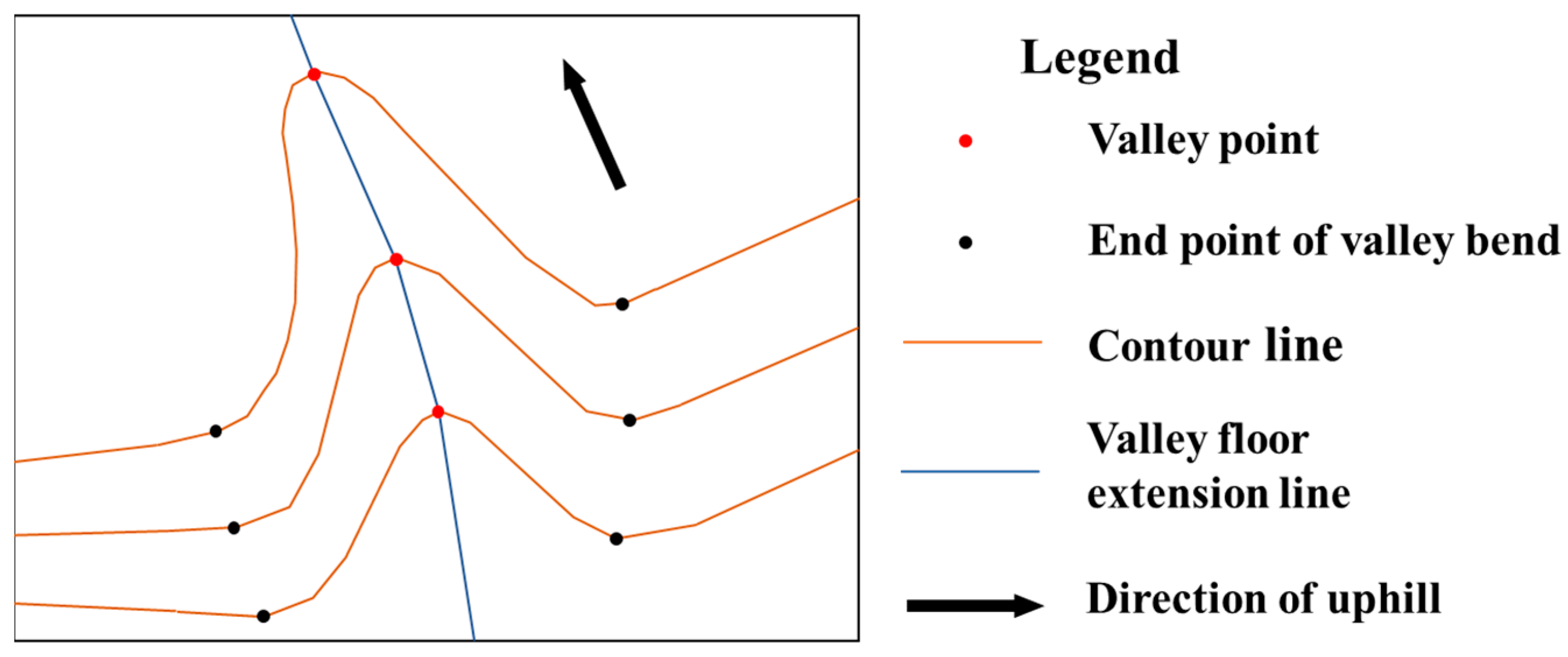
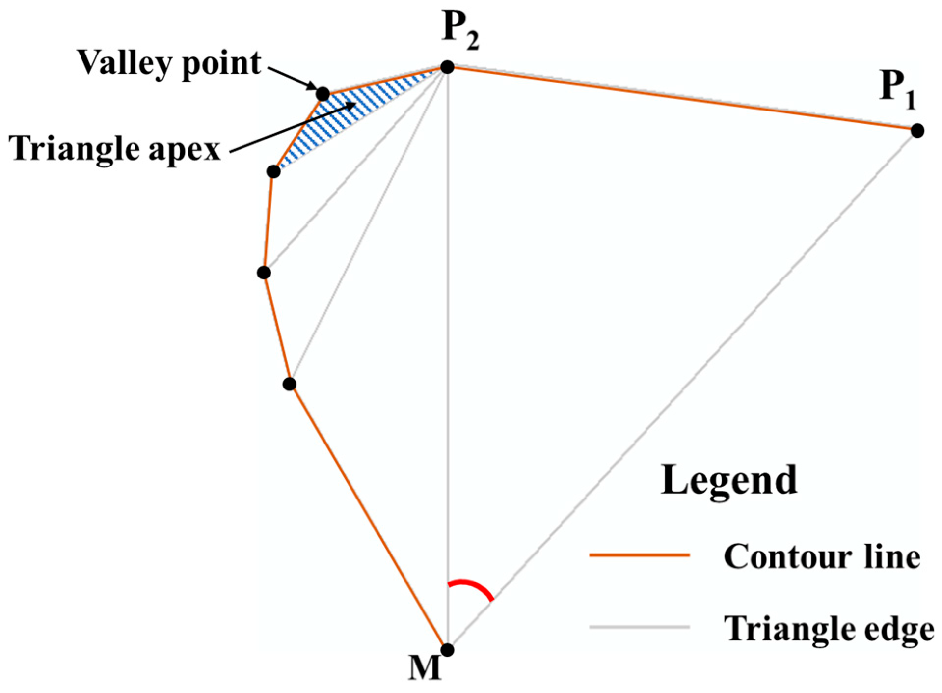
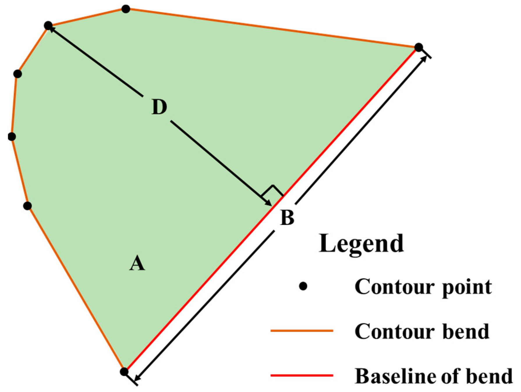
• The valley points were extracted based on the constrained DTN. The constrained DTN [19] was established in the valley bend, as shown in Figure 5. The line was connected by the two adjacent points $P_1$ and $P_2$ at the start of the bend as the starting baseline, and the third point $M$ found inside the bend, making $\angle P_{1}M{P}_2$ (colored red) the maximum angle. The first triangle, $P_{1}M{P}_2$, subsequently generated new triangles from both sides, with $P_{1}M$ and $M{P}_2$ as the baselines, until all the points had been processed. The vertex of the triangle apex (shaded with blue lines) is the valley point corresponding to the bend, as shown in Figure 5.
• Erroneous valley point correction. To find and correct erroneous valley points, we first calculated the curve coefficient of each point on the bend and defined the curve coefficient of point $P$ on the bend according to Equation (1):

  $$Cur(P)=\frac{\arccos \frac{P_{-l}P\cdot P{P}_{+l}}{\left|P_{-l}P\right|\left|P{P}_{+l}\right|}}{\left|P_{-l}P\right|\left|P{P}_{+l}\right|}$$

  (1)

  where $P_{-l}$ and $P_{+l}$ are two points on a contour line, with a path distance of $l$ on both sides of $P$. If the distance between the contour lines on this side was less than $l$, then the endpoint on this side of the contour line would substitute $P_{-l}$ or $P_{+l}$. Instead of using the traditional method, a certain length was used to intercept a curve segment of the contour line to calculate the curve coefficient [26,30].

The advantages of intercepting the contour line based on distance, rather than the point number, are as follows. The distance between adjacent points on a contour line may be unequal or vary considerably. This could result in substantial differences in the lengths of curve segments intercepted according to point number at the end of either side of the valley point. Therefore, the valley point would not be in the center of the intercepted curve, and the result would not reflect the curvature at the valley point. The length of the connecting line from the valley point to the endpoints of the intercepted sections of the contour line would be the same as the path distance if the intercepted section was completely straight. Otherwise, the lower the length, the greater the curvature of the contour section on that side. Using the product of the lengths of connecting lines on both sides as the denominator of the curve coefficient calculation better reflects the curvature at the valley point. The valley points extracted in Step (3) were evaluated based on whether they are replaced with a point with a large curve coefficient.

To overcome the over-reliance on point curvature for extracting valley points, it is necessary to limit the curve coefficient of the replacement point. The maximum curve coefficient corresponding to the valley points on the bend was assumed to be $Cu{r}_{F\max }$. We first used the algorithm introduced in Step (3) to extract the valley points from each bend. Based on observation of the incorrect valley points extracted in Step (3), we found that if the maximum value of the curve coefficient of points other than extracted those valley points on the bend where the they are located was greater than $5Cu{r}_{F\max }$, it was more effective to pass through this point when connecting the valley line. As a result, this point became the valley point. Otherwise, only the valley point with the largest curve coefficient was maintained.

Once they had been extracted, the valley points were screened to establish a candidate set of points of gradually descending valleys. At each valley point, two search lines, perpendicular to each other and with a length on both sides of $l_S$, were placed every 10° [31]. The number of contour lines intersected by the two search lines was then calculated. Based on the shape of the longisection, gradually descending valleys could be subdivided further into flat gradually descending valleys and deep gradually descending valleys. The elevation fluctuation of the longisection of a flat gradually descending valley was lower, the terrain on either side was flat, and they were mostly found on flat land in front of mountains. Feature points with zero intersecting search lines in each direction were marked as candidate valley points corresponding to a flat gradually descending valley. The elevation fluctuation of the longisection of a deep, gradually descending valley was greater. There was a considerable difference in slope between the direction of the valley and the direction perpendicular to it, and the number of contour lines intersected by the search lines in the two directions differed significantly. To limit the quantitative difference during the screening process, we used a logarithmic function with a low derivative value on $[1,+\infty )$ to manage the number of intersections of contour lines in the two directions, with the difference degree of intersection $\delta$ defined according to Equation (2).

$$\delta =\frac{\ln (n+\epsilon )}{\ln (m+\epsilon )}$$

(2)

where $m$ and $n$ are the lower and higher values of contour line intersections by the corresponding two search lines, respectively, and $\epsilon$ is the adjustment factor. As the logarithmic function was negative at $(0,1)$ and positive at $(1,+\infty )$, the value of $\epsilon$ was set at 1.1 to ensure that the numerator and denominator of the equation are always positive. When the difference in intersections increases in the denominator (the lower value of intersections), the numerator (the larger value of intersections) must increase by greater multiples for the ratio to remain the equal difference degree of intersection. This was a soft constraint on the smaller value of intersection to limit situations in which the value was too high and to ensure that the slope in this direction was small and was in the gradually descending direction. To further assess valley points with a maximum difference degree of intersection of more than 2, search lines with less and more intersections in this direction were recorded as $L_m$ and $L_n$, respectively. On a contour line with length $l_S$ on both sides of the point, if the distance on one side was less than $l_S$, the length in the opposite direction of the endpoint was extended until it was $l_S$. A method proposed by Xing et al. [32] was used to calculate the mean frontal projection distance $d_{proj}$ of the intercepted contour line and $L_n$. If it was greater than $0.4l_S$, and the curve coefficient at this valley point was greater than $\varsigma$, it meant that the contour line had greater curvature at this point, and the point was marked as a candidate valley point corresponding to a deep, gradually descending valley.

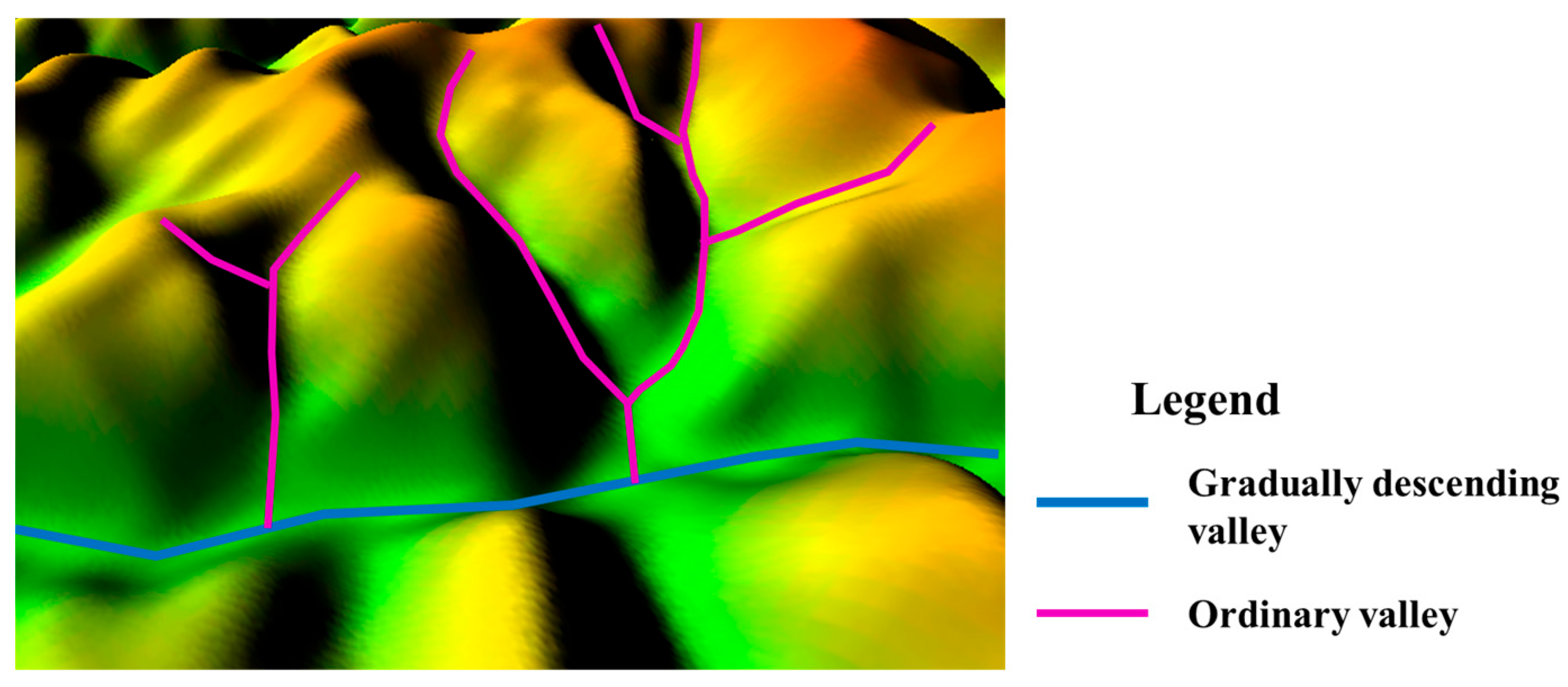
3.2. Valley Line Classification and Connection

After extracting and classifying the valley points, a set of candidate points of gradually descending and ordinary valleys was obtained. The process of connecting valley lines entailed, first, connecting the edges of gradually descending valleys and, subsequently, connecting ordinary valley lines under their control. To fully use the positional relationship between valley points, a DTN-based method was used to connect valley lines, with the contour line interval recorded as $\mathrm{\Delta }H$. A description of the specific process follows.

• Initial extraction of gradually descending valley edges. A Delaunay triangulation network (DTN) was established for all candidate points of gradually descending valleys, retaining edges, of which the height difference between two endpoints was $\mathrm{\Delta }H$ and the length was less than $6l_S$, as the initial set of gradually descending valley edges.
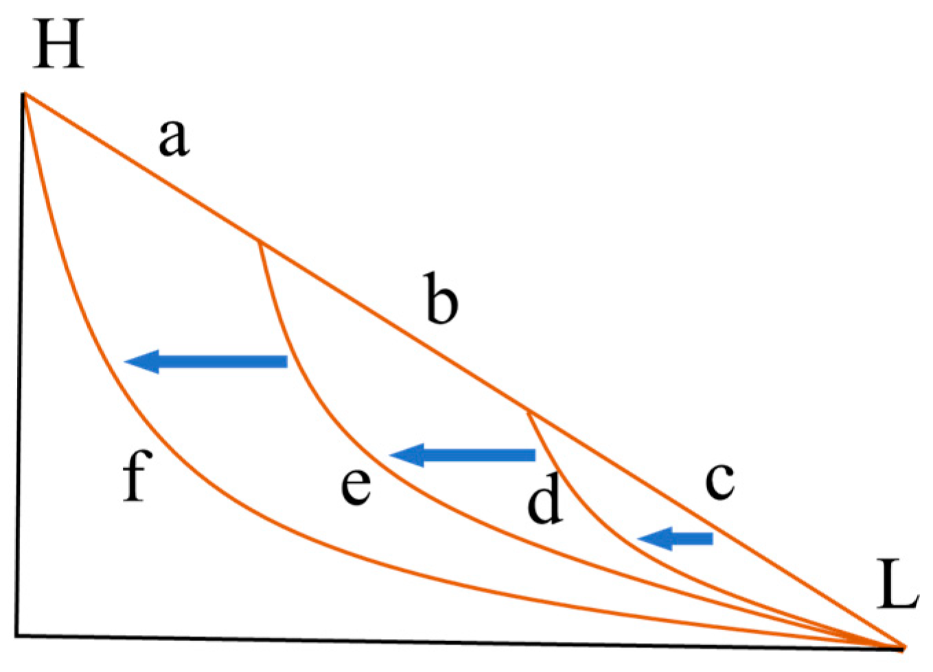
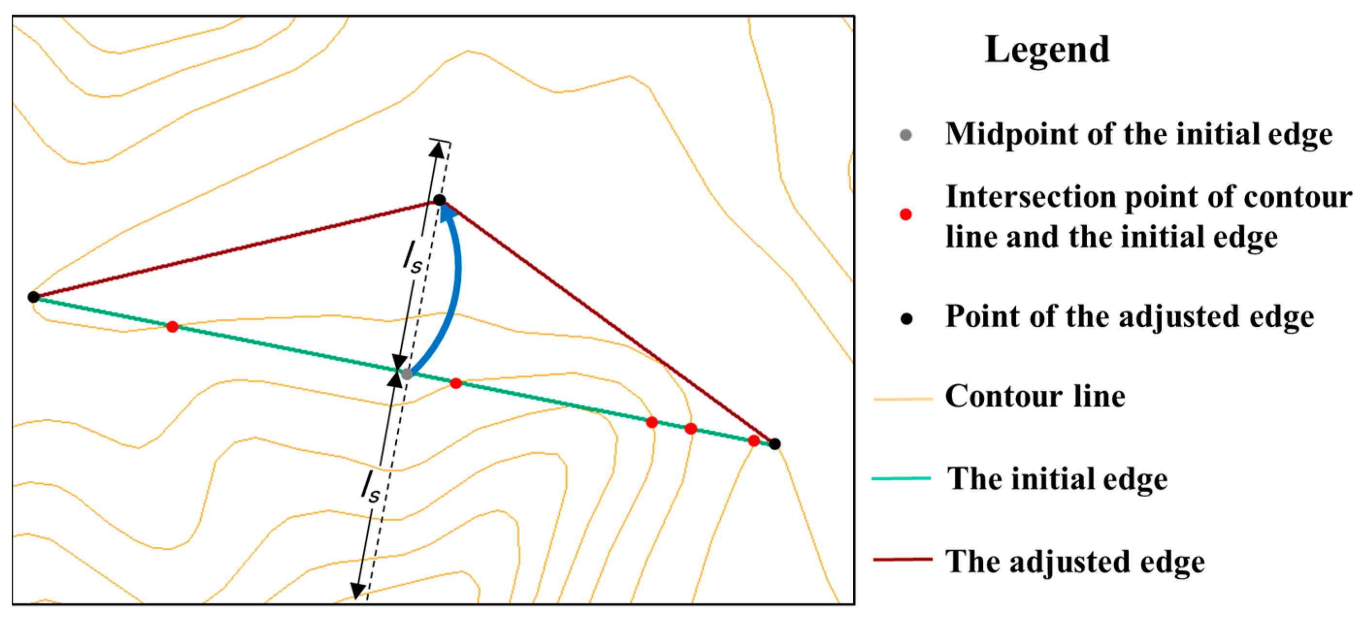
• Adjustment of gradually descending valley edges. The set of gradually descending valley edges was subsequently revised and screened to find the edge that intersected the contour line at the non-endpoint, a vertical bisector was drawn to that edge, and the midpoint of the edge was moved within the range $l_S$ at both sides until the edge did not intersect the contour line. If the condition could not be satisfied, regardless of the movement, the edge was deleted from the set of the gradually descending valley edges. In Figure 6, the green line is the edge of the gradually descending valley before adjustment, and the red points are the intersection points with the contour lines. After moving the midpoint along the vertical bisector in the direction of the blue arrow, the adjusted edges are represented by the purple lines.
• Supplementary connection of gradually descending valley edges. Supplementary connections were made to discontinuous points of the revised and screened edges of gradually descending valleys. The conditions for supplementary connections were as follows. The supplementary connection should only cross one contour line, with its elevation being between the contour lines at both ends of the connection, and the supplementary connection should be relatively straight. In the process of implementing, point $V$ was taken from the ordinary valley point set in turn, and the endpoints $V_1^L$ and $V_2^H$ of the two gradually descending valley edges were connected, namely $V_1^H{V}_1^L$ and $V_2^H{V}_2^L$, with $V$, where $V_{*}^H$ and $V_{*}^L$ represent the endpoints with higher and lower elevations of the valley edge, respectively. The elevation of $V$ should be $\mathrm{\Delta }H$ higher than that of $V_2^H$ and $\mathrm{\Delta }H$ lower than that of $V_1^L$. If $V_1^{L}V$ and $V{V}_2^H$ did not intersect contour lines except at endpoints, and $\angle V_1^{L}V{V}_2^H$ were greater than the included angle threshold $\alpha$, then $V_1^{L}V$ and $V{V}_2^H$ were added to the set of the gradually descending valley edges, thereby completing the extraction of the gradually descending valley edges. Jin and Gao [23] set the direction change angle threshold at 60° for connecting terrain feature lines, with the included angle corresponding to the supplementary angle of the direction change angle, implying the included angle threshold $\alpha$ was set to its supplementary angle of 120°.
• Preparation for the connection of ordinary valley lines. All the unconnected valley points of gradually descending valley edges were included in the set of ordinary valley points, and a Delaunay triangulation network was established for all the points included. The length of each edge was calculated, and the vector cross product was used to identify all the ridge bends and enveloping areas.
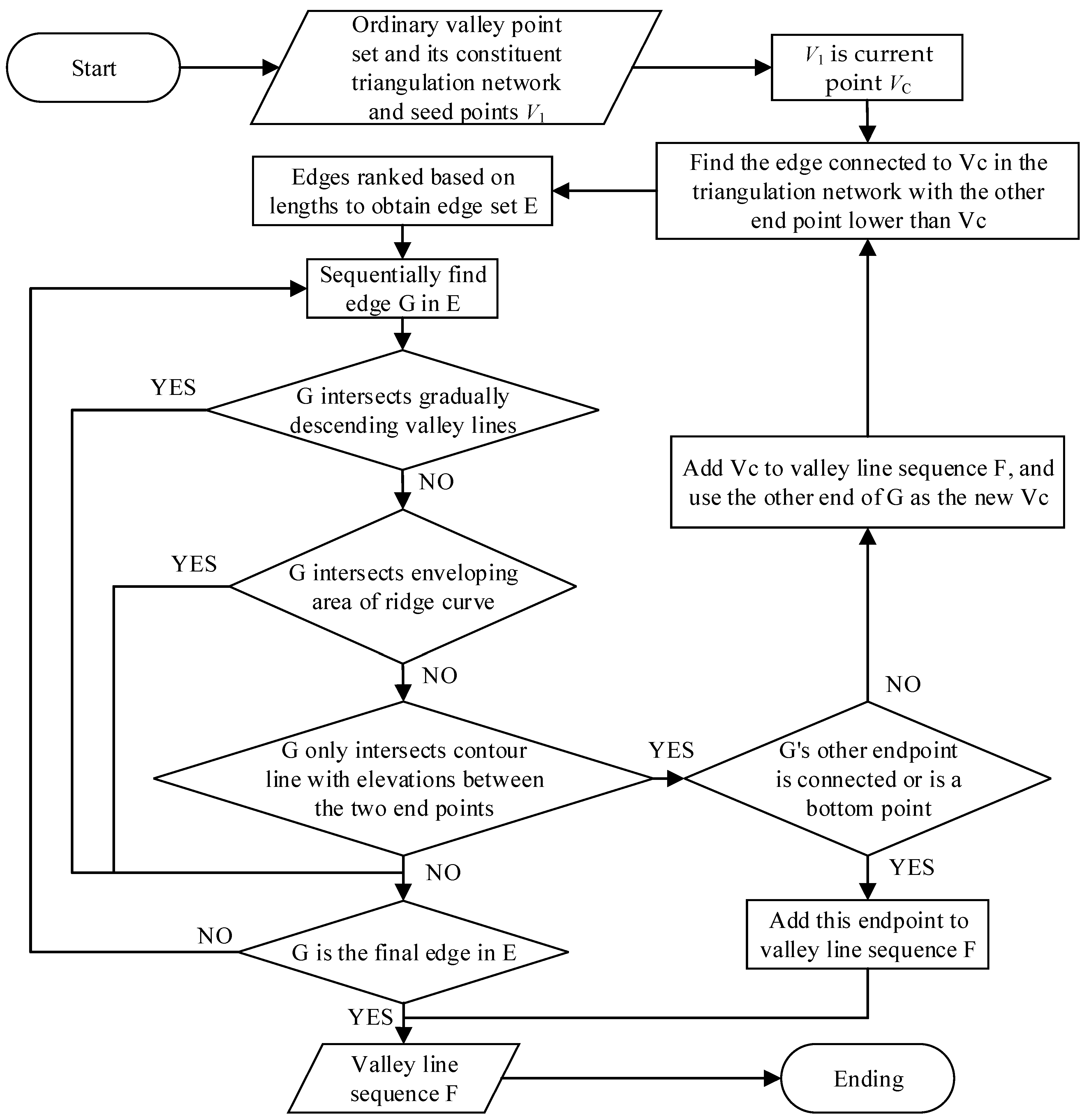
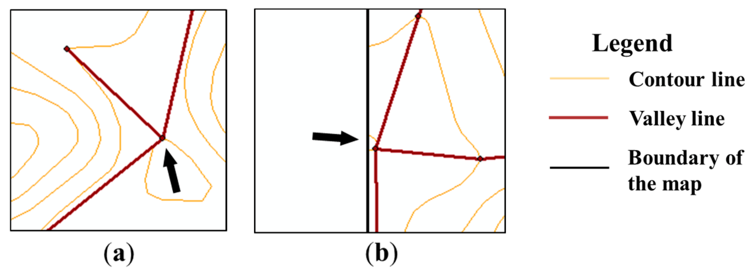
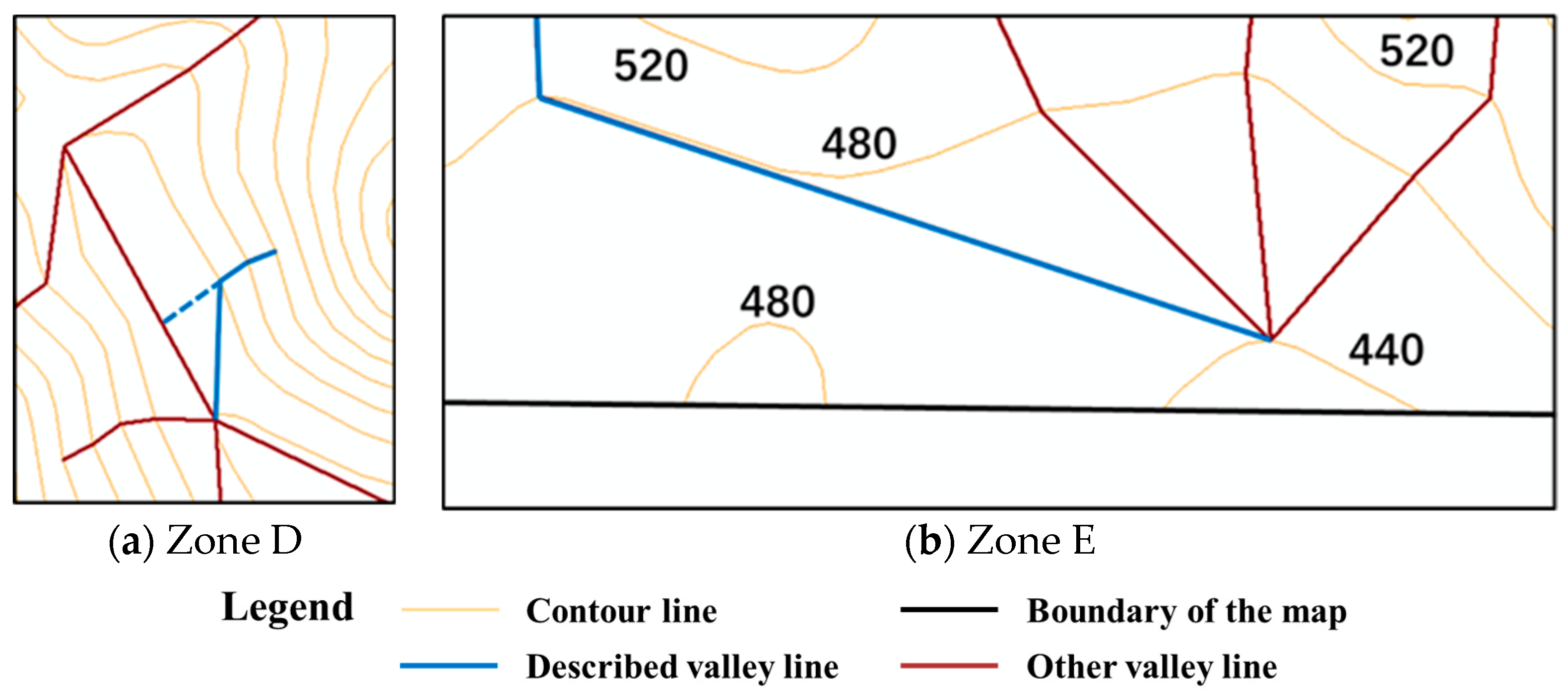
• Connection of ordinary valley lines. Ordinary valley points were sorted in descending order of elevation. Unconnected valley points were selected as seed points for valley line tracking. The workflow for processing each seed point $V_1$ is shown in Figure 7. The subsequent valley points to be connected were found individually by using specific filter conditions until the conditions for stopping the connections were met. Valley lines were tracked from the highest elevation first because water descends under the force of gravity after rainfall, with valleys formed by the mechanical movement of converging water along with decreases in elevation. Starting from the lowest elevation would lead to constantly encountering bifurcations, which would impede the tracking process. In geomorphology, it is accepted that a valley does not span other valleys or ridges. Therefore, edges that intersect with previously extracted gradually descending valleys and enveloping areas of ridge bends must be discarded. Given that surface water flows descend, the elevation of valley lines changes predictably. Therefore, the elevation of any point on each side of a valley line must be between the elevations of the endpoints on both sides. The conditions for stopping connections included traversing all edges connected to the current valley point and connecting to the bottom point or points already connected by other valley lines. The bottom point is the valley point with no other contour line inside the polygon formed by the closed contour line or the open contour line and the map margin, corresponding to the points indicated by the arrows in Figure 8a,b.
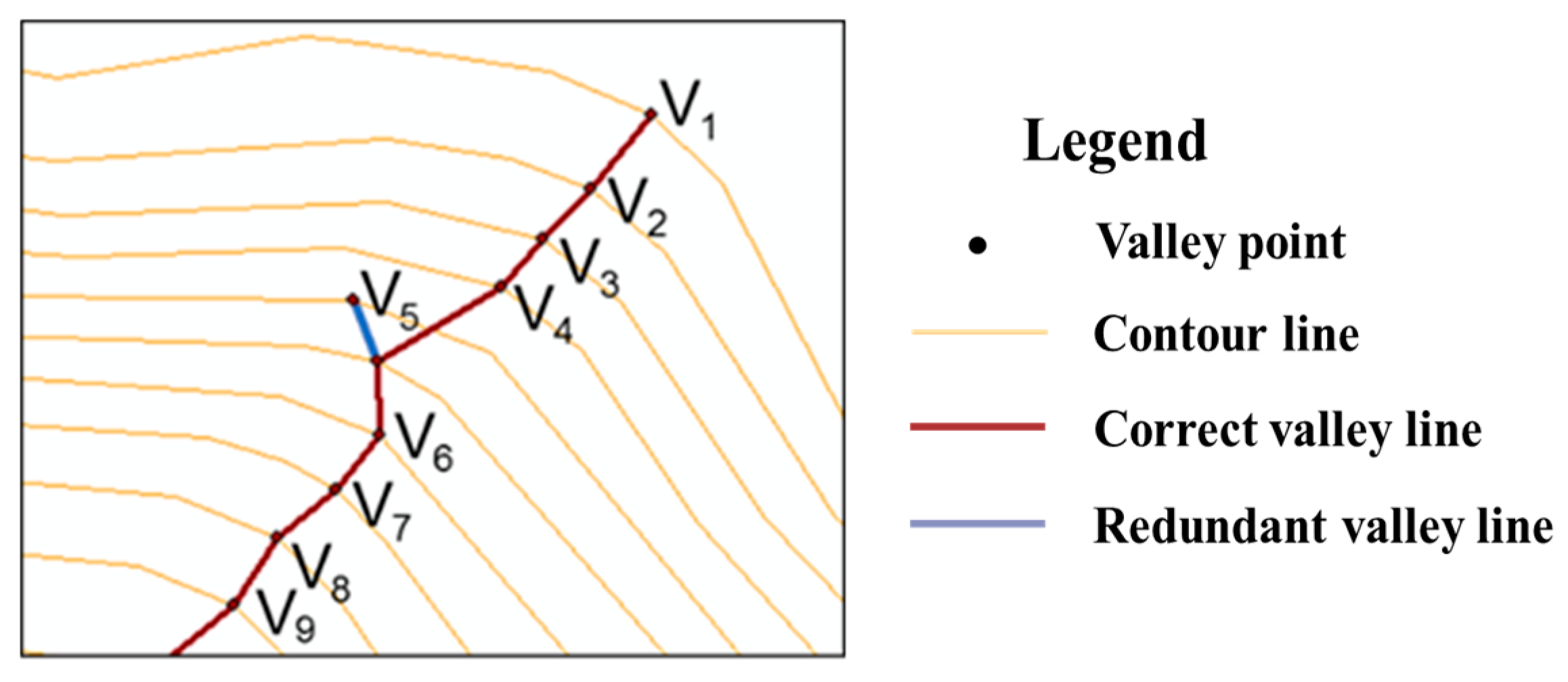
• Trimming redundant valley lines. Redundant valley lines occur when individual valley points have large deviation while edges generated by valley points in the Delaunay triangular network in Step (5) are being selected, leading to selection of a short line connecting a valley point on an adjacent contour line. When connecting this valley line, the current valley point would be crossed. This point was then used as a seed point to connect the adjacent lower valley point, generating a redundant valley line. Redundant valley lines appear as a small branch connected to a longer valley line. In Figure 9, $V_5$ is a valley point with a large deviation. The blue line is the redundant valley line corresponding to that point. Valley bends are used to represent the range of valley lines. If bends $b_1$, $b_2$, and $b_3$ intersected the valley line, its range would be $Range(v_1)=\{b_1,b_2,b_3\}$. For any valley line $v_i$, if $\exists v_k(k\ne i)$, $Range(v_i)\subset Range(v_k)$; therefore, $v_i$ would be designated as a redundant valley line and discarded.
• Supplementary connection of ordinary valley lines. Supplementary connections were made to the valley lines to form a complete tree structure between the lines. If the valley point with the lowest elevation on an ordinary valley line was not connected to other valley lines and it was not a bottom point, connections were attempted with all the lower valley points through this point. If a connecting line did not intersect the contour line and valley line, it was added to the current valley line; otherwise, no action was taken.
• The obtained ordinary valley lines were smoothed to meet human cognition. For the three consecutive points $V_{i-1}$, $V_i$, and $V_{i+1}$ on the valley line, the inner point of the bend where $V_i$ is located was determined. If point $V_i{}^{\prime }$ was on the same bend as $V_i$ and $\angle V_{i-1}{V}_i{}^{\prime }{V}_{i+1}>\angle V_{i-1}{V}_i{V}_{i+1}$, $V_i$ was subsequently replaced with $V_i{}^{\prime }$. The point sequence of the valley line was updated simultaneously until the entire valley line was processed.

3.3. Contour Line Group Simplification

In an area with predominantly positive landforms, the group of valley bends must be processed. Contour line simplification is conducted according to the geometric features of the valley and its position in the valley network by selecting the corresponding group of bends. Valley lines extend downward from the highest point and converge to form a tree-like structure. For all valley lines converging at the same point, the valley line with the highest status is the one with the highest starting elevation. If the starting elevations of multiple valley lines were the same, the longest one was considered the highest.

Three indicators of the geometric features of valleys were selected, namely the length of the baseline of bend $B$, depth of bend $D$, and area of bend $A$ as shown in Figure 10. The length of the bend baseline refers to the distance between the two endpoints of the bend. The depth of the bend is the maximum distance from the points on the bend to the baseline. The area of the bend is the area of the closed polygon comprising the bend and its baseline. The bend area was considered the most important indicator because it intuitively expresses the visual significance of a bend on a map. However, situations could arise in which the area satisfied the selection criteria, but the gap between the horizontal and vertical lengths was so substantial that it was difficult to clearly represent the shorter side on the map. Therefore, two additional indicators of baseline length and depth were required to identify bends with horizontal or vertical lengths below the thresholds. Moreover, considerable computation was required to calculate the bend area; therefore, these two indicators were calculated first. If the threshold was not reached, it was deleted, and there was no need to calculate the bend area.

Given that gradually descending valleys are often important in large-scale maps, all these valleys were retained during simplification. Traversing the ordinary valley, all bends with a feature line through them were identified and their status was determined. Subsequently, all valley lines that passed through the lowest elevation endpoint were identified. If the endpoint contained a gradually descending valley or a higher-status valley, the bend where the endpoint was located was skipped in the bend group selection process. Otherwise, the continuity of the corresponding bend group of gradually descending or higher-status valleys would be negatively affected. The maximum values of the three geometric indicators ($B_{\max }$,$D_{\max }$, and $A_{\max }$) were subsequently found in the bend group. If one of them was below their corresponding threshold ($B_t$, $D_t$, and $A_t$), then the original bend was replaced by the corresponding baseline. This was the case because the most visually striking bend in the bend group was the one with the largest geometric indicators. Further, the loss of graphic information caused by deleting the bend would be the most significant of the entire bend group. If one of the three geometric indicators had not reached the threshold, the consequence of deleting this bend was considered acceptable, and the consequences of deleting other bends in the group were also considered acceptable. Therefore, it was used as the indicator for selecting the bend group.

4. Experiments and Analysis

4.1. Experiment Data and Pre-Processing

We tested our proposed methodology with contour line data containing 270 contour lines from an area of Henan Province, China, at a scale of 1:50,000, with an elevation interval of 20 m. The contour line data included attribute information such as contour line ID, elevation, and whether contour lines were closed. The scale of the target map was 1:100,000, with an elevation interval of 40 m, and it contained 139 contour lines after selection according to elevation. The size of the test zone area was 186.848 km² and it was a typical fluvial landform dominated by low- and middle-elevation mountains. The maximum and minimum contour line elevations were 1420 m and 360 m, respectively. To verify the effectiveness of the method proposed in this study, the algorithm was implemented using free Anaconda Notebook 5.7.8 distribution software (Anaconda, Austin, TX, USA) to search and install Python/R (Python organization, VA, USA).

The smallest gap clearly shown on the map was 0.2 mm [33]. According to the principle of the Douglas–Peucker algorithm, the distance from the original contour line on either side of the simplified contour line to it is less than the threshold of the algorithm. Therefore, the distance of wavers on the origin contour line are less than twice the threshold of the algorithm in the direction perpendicular to the simplified contour line. On this basis, we used half of this gap to define a small waver in the contour lines, with a corresponding distance on the target-scale map of 10 m. Contour lines were pre-processed using the Douglas–Peucker algorithm, with a threshold of 10 m to prevent wavers from affecting the identification of valley points.

4.2. Test Results and Comparative Analysis

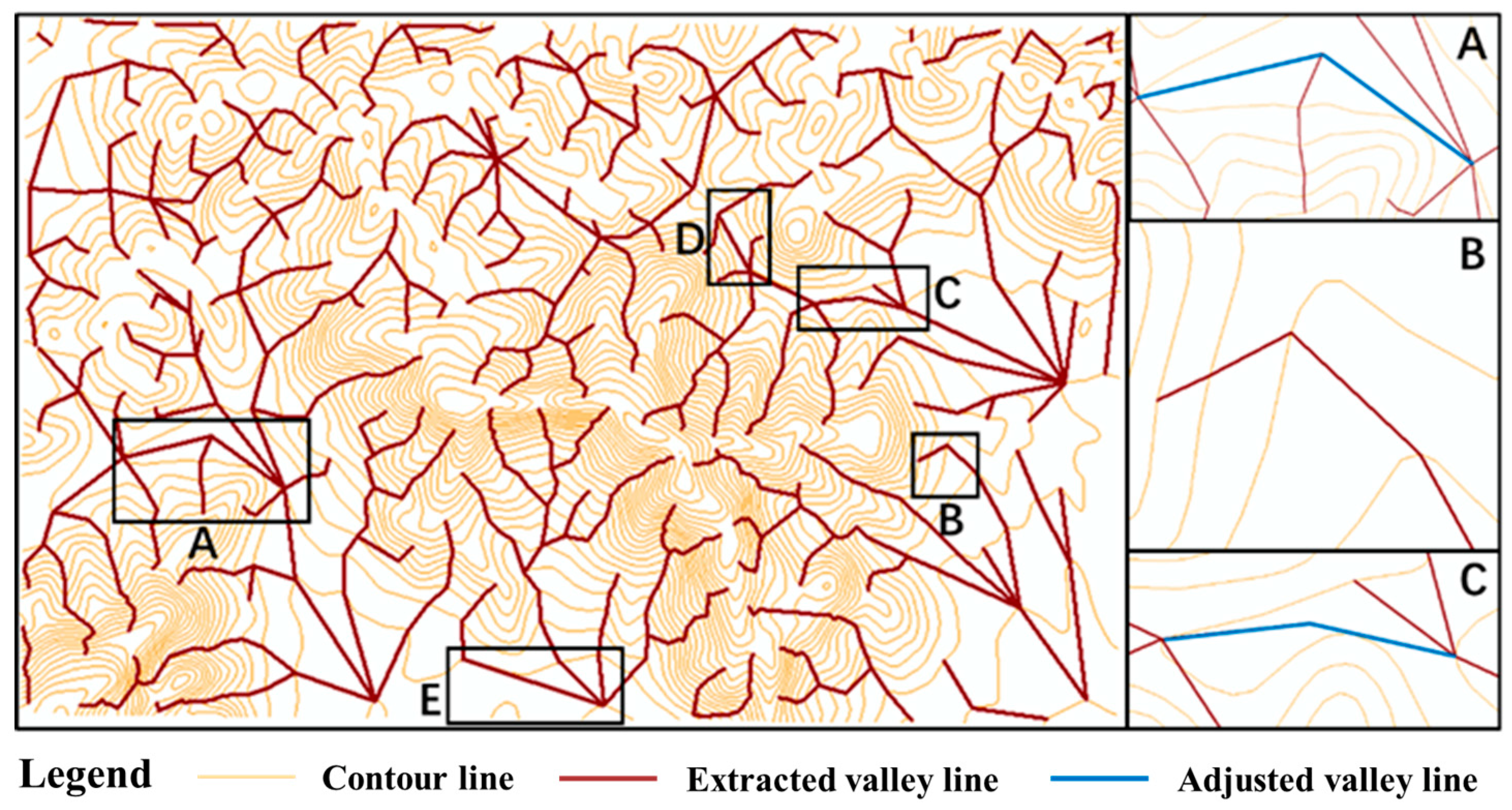
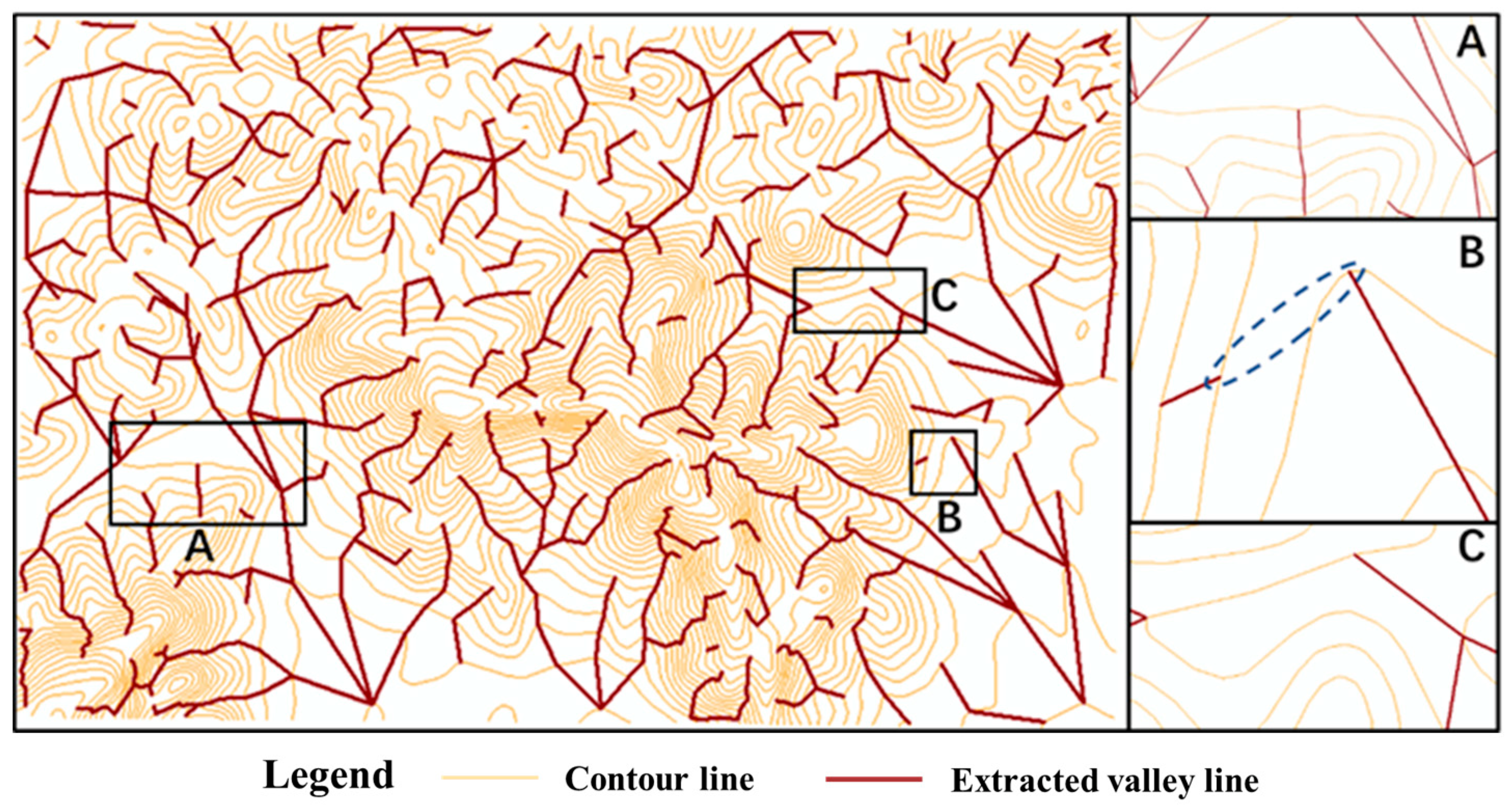
4.2.1. Valley Line Extraction Results and Analysis

We compared the valley line extraction algorithm proposed in this study with the method presented by Zhang et al. [19] (Figure 11 and Figure 12), in which thin lines are contour lines and thick lines are valley lines. Jin and Gao [23] set the length of search lines to 12 times the elevation interval when determining the type of extracted terrain feature points. According to the authors, this step effectively improved the efficiency of the algorithm while maintaining its efficacy. In our study, the length of a single side of search line $l_S$ was set in the same way and then rounded up to 500 m. Sampling length $l$ for calculating the curve coefficient was set as the mean distance between adjacent points on the contour line after pre-processing (150 m in this experiment) to prevent an excessive distance between the points on both sides. Turning angle $\beta =1rad$ was used to define the curve coefficient threshold $\varsigma$ for deep, gradually descending valley bends, as shown in Equation (3).

$$\varsigma =\frac{\beta }{l^2}$$

(3)

We substituted the corresponding parameters into the calculation, with a curve coefficient threshold $\varsigma$ of $4.4\times {10}^{-5}rad/m^2$. The method proposed by Zhang et al. [19] effectively extracts valley lines from contour lines. In most areas, relatively complete valley lines could be extracted and automatically connected to form a tree structure with abundant extracted information. However, as this method involves only graphics processing, the extraction results of some valley lines could differ from those perceived by an observer. However, our proposed algorithm used the natural geographic features of valley development as its starting point and fully considered the features of gradually descending valleys and ordinary valleys. Premised on fully retaining topographic details, our algorithm improves the integrity and structure of valley line connections, i.e., they were made to closely match human perception.

The deep gradually descending valleys located in Zones A and C (Figure 11 and Figure 12) turn at relatively large angles, with significant differences in the distances between adjacent contour bends. The similarities between the bends of the gradually descending valleys were not as clear as those in most other zones. The blue lines in the enlarged images in Figure 11 are valley lines extracted by our proposed algorithm and are closely matched to human perception, whereas the same locations are not connected with the use of other methods, as shown in Figure 12. This finding indicated that the method proposed by Zhang et al. [19] is not well-suited to deep, gradually descending valleys with complex contour line delineations. In zone B (Figure 11 and Figure 12), there was little depth at the start of the valley and the corresponding contour bend depth was small. The figure shows that the depth increases significantly as the valley descends. The blue dotted circle in the enlarged image of zone B (Figure 12) highlights that the results extracted using the Zhang et al. method [19] did not create a connection here. However, the method proposed in our study successfully identified the relationship and made the connection, thereby maintaining the integrity and structure of the valley line.

The valley line extraction algorithm proposed in this study was intended for cartographic generalization. Given that the core objective was to group contour bends using valley lines, retaining the intersecting relationship between the valley lines and corresponding bends was a crucial factor. However, the result lacked visual effect. Figure 13a shows an enlarged view of Zone D from Figure 11. The last section of the valley line, indicated by the blue line, is connected in the direction of the dotted line, which is close to that perceived by humans. However, by using this connection method, the valley line fails to pass through the bottom bend, making it difficult to represent the subsequent bend relationship. Therefore, it was necessary to use the solid line in the figure for connecting it with a large turning point to clarify the relationship between the valley line and the bend when the contour lines were grouped. Figure 13b shows an enlarged view of zone E in Figure 11. The contour line information near the map border is not sufficiently detailed, and the valley line represented by the blue line forms a tree structure, also with a large turn.

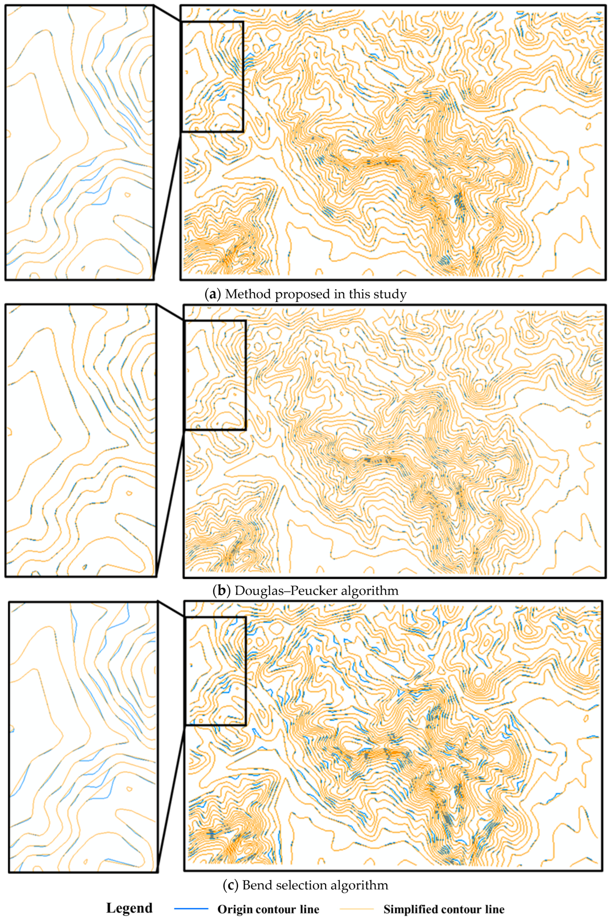
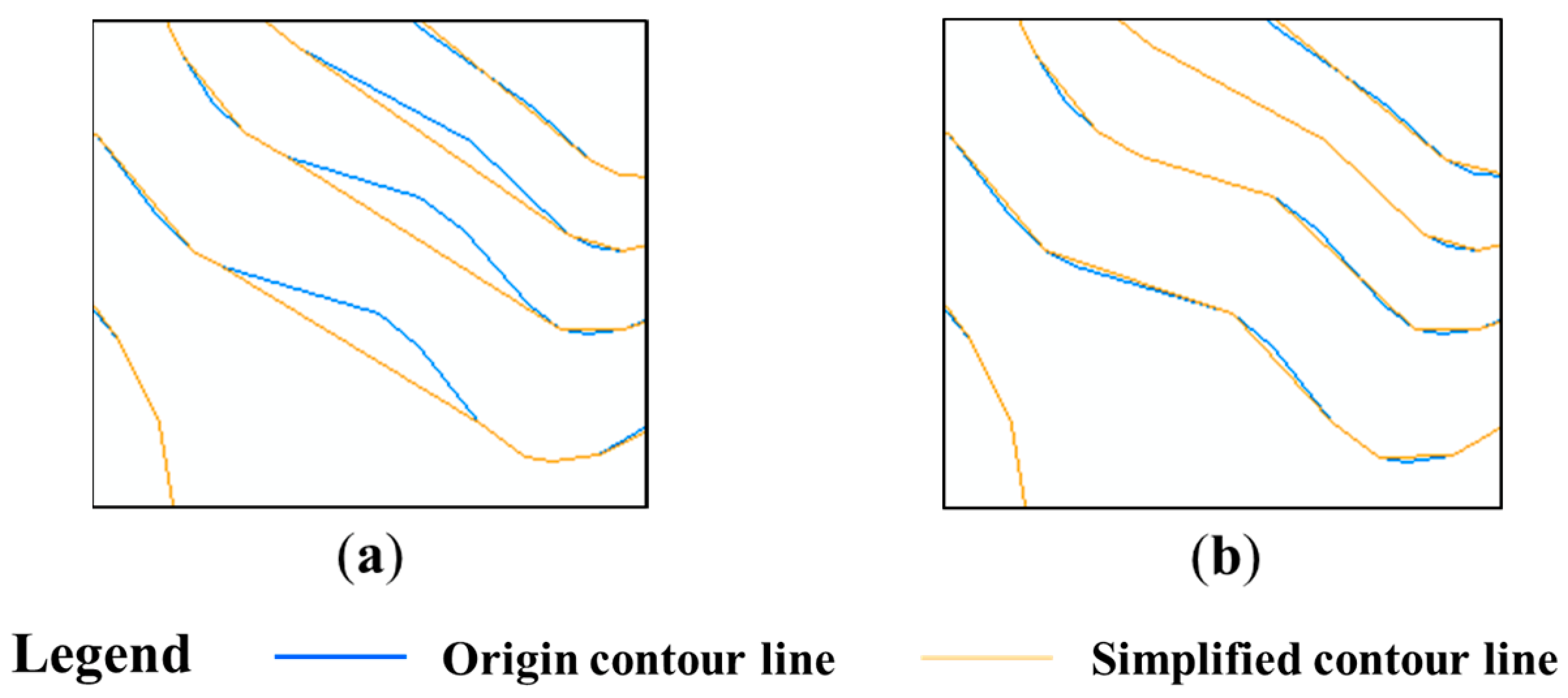
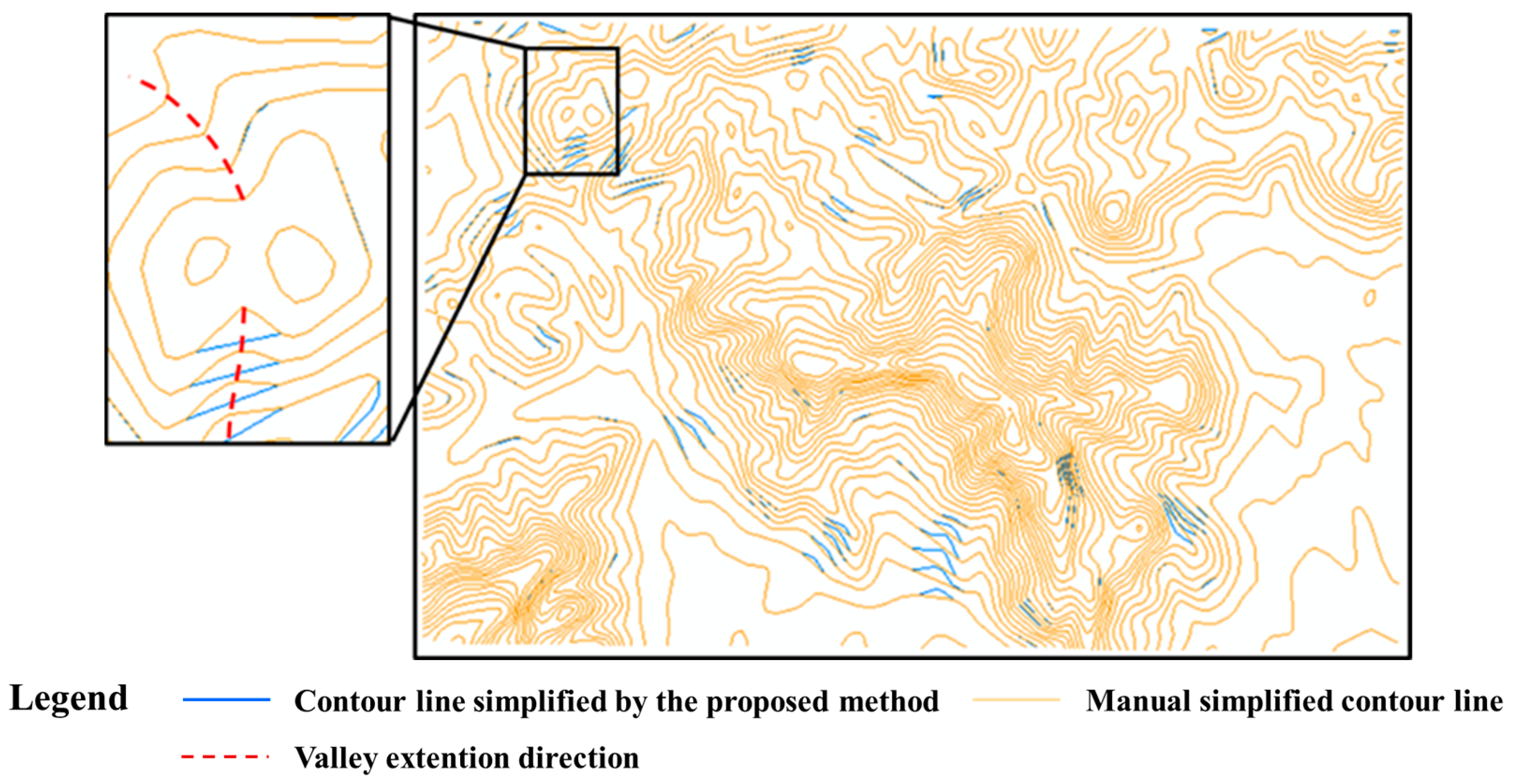
4.2.2. Results and Analysis of Contour Line Simplification

We conducted a comparison between our proposed method and the Douglas–Peucker [3] and bend selection algorithms. The bend identification method of Zhu et al. [8] was employed for the bend selection algorithm, with the bend area as the indicator. Regarding the parameter settings for contour line simplification, as the smallest visible target on the map was 0.3–0.5 mm [4], the length of a bend baseline was considered the distance between two points that objectively existed on the map, which could be perceived more easily. In this study, parameter $B_t$ was set as the distance corresponding to the lower limit of the scale range of the target-scale map, which was 30 m. Parameter $D_t$, corresponding to the bend depth, was set as the distance corresponding to the upper limit of the scale range of the target-scale map, which was 50 m. The area threshold $A_t$ was considered the most important parameter, as it plays a leading role in the degree of simplification. The higher the threshold, the fewer bend groups can reach it, and the more bends are then deleted. The square root model [34] is the most popular and widely accepted for determining the information amount of a map. After several tests, we found that when the value was 40,000 m², 116 of the 171 valleys in the experimental area were retained, with a retention ratio of 67.84%. This was close to the retention ratio of 70.71% calculated using the square root model based on the scales before and after simplification. To achieve simplification approximately equal to that of our method, the parameter of the Douglas–Peucker algorithm was set to 12 m and that of the bend selection algorithm was set to 40,000 m². The results are shown in Figure 14. The blue lines are contour lines before simplification, and the yellow lines are contour lines after simplification.

Three indicators were used to quantitatively assess the results of the three algorithms: point compression, horizontal deviation, and visible valley bend reduction (

Table 1. Evaluation of contour line simplification results.

Algorithm	Point Compression (%)	Horizontal Deviation (m/km)	Visible Valley Bend Reduction (%)
Method proposed in this study	20.22	23.537	6.33
Douglas–Peucker algorithm	25.88	21.042	2.11
Bend selection algorithm	18.83	62.351	20.53

). Higher point compression [11] equated to a higher degree of simplification. Horizontal deviation was the ratio of the mean frontal projection distance [32] to the length of the contour line before simplification. The lower the value, the smaller the deviation of the simplified contour line. The visible valley bend reduction rate was measured using the ratio of valley bends, of which the baseline length and depth were greater than 0.5 mm on the map [4], before and after simplification.

When comparing the point compression rate, the performances of the three algorithms were similar; however, the degree of simplification of the Douglas–Peucker algorithm was slightly higher than that of the other two methods. In terms of horizontal deviation, our proposed method had a notably smaller deviation after simplification than that of the bend selection algorithm, and its performance was similar to that of the Douglas–Peucker algorithm. In terms of visible valley bend reduction, the result from our method was three times higher than that of the Douglas–Peucker method, implying that, although the reduction of visual information on the map was stronger, it was weaker than that of the bend selection algorithm. Figure 15 shows a visual comparison of the simplification results of the algorithm method proposed in this study and the Douglas–Peucker algorithm for a group of small-scale valley bends. Our method achieved group simplification, effectively reducing map information, and the obtained contour line fit was effective. The Douglas–Peucker algorithm can only be used to delete small waves on contour lines. However, it cannot be used to delete entire bends. Therefore, the visible information on the map cannot be effectively reduced after simplification. Figure 16 shows the results of our method and the bend selection algorithm for another area. The red dotted line indicates the valley direction. The aim of group simplification is to realize terrain simplification, rather than graphical simplification. The simplification result of our proposed method preserved the bends that the valley passes through, whereas the bend selection algorithm deleted parts of the bends, undermining the integrity of the terrain structure. Therefore, the simplified contour lines obtained using our proposed method were the most effective at retaining the structural features of the original topography. This demonstrates the advantage of the group simplification method.

To assess the effectiveness of our proposed method, we compared its results with those of manual simplification (Figure 17). The yellow lines in the figure are the contour lines obtained by manual simplification and the blue lines are the inconsistencies identified using the simplification method proposed in this study. We used the visual buffer tolerance method [35] to quantitatively assess the similarities between the two methods, with 0.2 mm on the map as a radius to establish a buffer zone for the contour lines obtained by manual simplification. The visual buffer tolerance was defined as the ratio of the length of a contour line in the buffer zone obtained by our proposed simplification method to its total length. The buffer tolerance of the two results was calculated as 97.37%, indicating that the contour lines obtained using the two methods were highly similar. The manual process considers more complex factors such as the density of terrain structures and their relationship, whereas our proposed method only considers the characteristics of the valley bend group, leading to some differences in the simplification results. In the areas where the valleys are relatively dense, more valley bend groups were deleted using manual processes than using our proposed methods, and vice versa. In this way, the ratio of the valley densities can be maintained after simplification using manual processes. In the enlarged image in Figure 17, the two red dotted lines are the direction of two valleys of a saddle. The method in this study deleted the bend group of one of the valleys and failed to consider the relationship between the two valleys.

In summary, the method proposed in this study effectively extracted valley lines and overcame the shortcomings of traditional methods regarding the identification of gradually descending valleys. Our method successfully formed valley line networks with acceptable structural integrity, according to the principles of human perception, and which could be applied to the grouping of contour bends. Our group simplification method has, therefore, been shown to achieve reliable results. At approximately the same degree of simplification, the results of our method were highly similar to those of manual simplification. The results produced by the proposed method maintained a small horizontal deviation, effectively reduced map information, and retained the structural features of the original terrain. However, our proposed method could not account for the influence of relationships between terrain structures on contour line simplification.

5. Conclusions

This study introduced a contour line group simplification method based on terrain structure lines. The first step was to extract valley points and classify them into two types: gradually descending valley candidate points and ordinary valley points. Subsequently, the feature lines of both types of valleys were connected. Finally, contour lines were grouped by extracted valley lines and selected according to the geometric indicators of the bend group, thereby achieving simplification of the contour line groups. Our results indicated that the proposed method could effectively extract valley lines from contour lines and connect them to form a tree-shaped valley network. It also effectively achieved group simplification of contour lines with few deviations from the original contour lines, good retention of terrain structure features, and results comparable to those of manual simplification.

Future research should focus on improving the connection method of valley line classification and the extraction algorithm to better align with the principles of visual perception and facilitate their use in other fields such as hydrology. Furthermore, the relationships between terrain structures should be used as a key reference element in contour line grouping and simplification to produce results that are close to those of manual compilation and to satisfy the requirements of practical applications.

References

1. Tang, G.; Na, J.; Cheng, W. Progress of digital terrain analysis on regional geomorphology in China. Acta Geod. Et Cartogr. Sin. 2017, 46, 1570–1591. [Google Scholar]
2. Wu, F.; Gong, X.; Du, J. Overview of the research progress in automated map generalization. Acta Geod. Et Cartogr. Sin. 2017, 46, 1645–1664. [Google Scholar]
3. Douglas, D.H.; Peucker, T.K. Algorithms for the reduction of the number of points required to represent a digitized line or its caricature. Can. Cartogr. 1973, 10, 112–122. [Google Scholar] [CrossRef] [Green Version]
4. Li, Z.; Openshaw, S. Algorithms for automated line generalization based on a natural principle of objective generalization. Int. J. Geogr. Inf. 1992, 6, 373–389. [Google Scholar] [CrossRef]
5. Visvalingam, M.; Whelan, J.C. Implications of weighting metrics for line generalization with Visvalingam’s Algorithm. Cartogr. J. 2016, 53, 253–267. [Google Scholar] [CrossRef]
6. Tutić, D.; Štanfel, M.; Jogun, T. Automation of cartographic generalisation of contour lines. In Unbounded Mapping of Mountains, Proceedings of the 10th ICA Mountain Cartography Workshop, Berchtesgaden, Germany, 11 July 2016; Technische Universität Dresden, Institute of Cartography: Dresden, Germany, 2016; pp. 65–77. [Google Scholar]
7. Qian, H.; Zhang, M.; Wu, F. A new simplification approach based on the Oblique-Dividing-Curve Method for Contour Lines. ISPRS Int. J. Geo-Inf. 2016, 5, 153. [Google Scholar] [CrossRef] [Green Version]
8. Zhu, Q.; Wu, F.; Qian, H.Z. Cognizing and structuring valley curves of contour lines based on the idea of subdivision. J. Geomatics Sci. Technol. 2014, 31, 424–430. [Google Scholar]
9. Mozas-Calvache, A.T.; Urena-Camara, M.A.; Percz-Garcia, J.L. Accuracy of contour lines using 3D bands. Int. J. Geogr. Inf. Sci. 2013, 27, 2362–2374. [Google Scholar] [CrossRef]
10. Gokgoz, T. Generalization of contours using deviation angles and error bands. Cartogr. J. 2005, 42, 145–156. [Google Scholar] [CrossRef] [Green Version]
11. He, G.; Zhang, X.; Sun, Y.; Luo, G.; Chen, L. Contour line simplification method based on the two-level Bellman–Ford algorithm. Trans. GIS 2020, 25, 396–423. [Google Scholar] [CrossRef]
12. Zheng, Y.; Zhang, L.; Guilbert, E.; Longa, Y. An improved spatial contour tree constructed method. Proc. Int. Cartogr. Assoc. 2018, 1, 128. [Google Scholar]
13. Ai, T. The drainage network extraction from contour lines for contour line generalization. ISPRS J. Photogramm. Remote Sens. 2007, 62, 93–103. [Google Scholar] [CrossRef]
14. Yang, Z.; Liu, G. Progressive graphical simplification of contour lines based on topographical feature constraints. In Proceedings of the International Conference on Intelligence Science and Information Engineering, Wuhan, China, 20–21 August 2011; pp. 181–184. [Google Scholar]
15. Lan, Y.; Cheng, Y.; Liu, X. Research and implementation of contours automatic generalization constrained by terrain line. In Big Data Analytics for Cyber-Physical System in Smart City. Advances in Intelligent Systems and Computing; Atiquzzaman, M., Yen, N., Xu, Z., Eds.; Springer: Singapore, 2020; pp. 707–713. [Google Scholar]
16. Huang, L.; Fei, L. Experimental investigation on the three dimension generalization of contour lines using 3D D-P Algorithm. Geomat. Inf. Sci. Wuhan Univ. 2010, 35, 55–58. [Google Scholar]
17. Dou, S.; Zhang, X. The improvement of the three dimensional Douglas–Peucker Algorithm. Adv. Mater. Res. 2014, 926–930, 3701–3704. [Google Scholar]
18. Cheng, L.; Guo, Q.; Fei, L.; Wei, Z. An improved integrated generalization method for contours and rivers using importance sequence of all points from these two elements. Geocarto Int. 2021, 36, 1–16. [Google Scholar] [CrossRef]
19. Zhang, Y.; Fan, H.; LI, Y. A method of terrain feature extraction based on contour. Acta Geod. et Cartogr. Sin. 2013, 42, 574–580. [Google Scholar]
20. Aumann, G.; Ebner, H.; Tang, L. Automatic derivation of skeleton lines from digitized contours. ISPRS J. Photogramm. Remote Sens. 1991, 46, 259–268. [Google Scholar] [CrossRef]
21. Ai, T.; Yang, M.; Zhang, X.; Tian, J. Detection and correction of inconsistencies between river networks and contour data by spatial constraint knowledge. Cartogr. Geogr. Inf. Sci. 2014, 42, 79–93. [Google Scholar] [CrossRef]
22. Liu, H.; Jin, H.; Miao, B. An algorithm for extracting terrain structure lines based on contour data. In Proceedings of the SPIE-The International Society for Optical Engineering, Beijing, China, 18–20 October 2010; 7840, pp. 286–291. [Google Scholar]
23. Jin, H.; Gao, J. Research on the algorithm of extracting ridge and valley lines from contour data. Geo. Spat. Inf. Sci. 2012, 8, 282–286. [Google Scholar]
24. Li, C.; Guo, P.; Wu, P.; Liu, X. Extraction of terrain feature lines from elevation contours using a directed adjacent relation tree. ISPRS Int. J. Geo-Inf. 2018, 7, 163. [Google Scholar] [CrossRef] [Green Version]
25. Zheng, X.; Xiong, H.; Gong, J.; Yue, L. A robust channel network extraction method combining discrete curve evolution and skeleton construction technique. Adv. Water. Resour. 2015, 83, 17–27. [Google Scholar] [CrossRef]
26. Guo, Q.; Yang, Z.; Feng, K. Extracting topographic characteristic line from contours. Geomat. Inf. Sci. Wuhan Univ. 2008, 33, 253–256. [Google Scholar]
27. Li, C.; Guo, P.; Liu, X.; Yin, J.; Zhang, C. The method of adjacent relation judgment and automatic direction adjustment of contour. In Proceedings of the 25th International Conference on Geoinformatics, Buffalo, NY, USA, 2–4 August 2017; pp. 1–5. [Google Scholar]
28. Raposo, P.; Touya, G.; Bereuter, P. A change of theme: The role of generalization in thematic mapping. ISPRS Int. J. Geo-Inf. 2020, 9, 371. [Google Scholar] [CrossRef]
29. Yan, Q.; Zeng, Z. Geomorphology; Higher Education Press: Beijing, China, 1985. [Google Scholar]
30. Guo, W.; Yu, A.; Sun, Q.; Li, S.; Xu, Q.; Wen, B.; Li, Y. A multisource contour matching method considering the similarity of geometric features. J. Geod. Geoinf. Sci. 2020, 3, 76–87. [Google Scholar]
31. Cheng, M.; Sun, Q.; Kang, S.; Chen, H.; Yang, N.; Li, C. Direction relation matrix model considering the location characteristics. J. Phys. Conf. Ser. 2022, 2224, 012060. [Google Scholar] [CrossRef]
32. Xing, R.; Wu, F.; Zhang, H.; Gong, X. Dual-carriageway road extraction based on facing project distance. Geomat. Inf. Sci. Wuhan Univ. 2018, 43, 152–158. [Google Scholar]
33. Wang, J.; Sun, Q.; Wang, G.; Jiang, N.; Lyu, X. Principles and Methods of Cartography, 2nd eds; Science Press: Beijing, China, 2014. [Google Scholar]
34. Topfer, F.; Pillewizer, W. The principles of selection. Cartogr. J. 1966, 3, 10–16. [Google Scholar] [CrossRef]
35. Du, J.; Wu, F.; Xing, R.; Gong, X.; Yu, L. Segmentation and sampling method for complex polyline generalization based on a generative adversarial network. Geocarto Int. 2021, 37, 4158–4180. [Google Scholar] [CrossRef]
Figure 1. Water erosion evolution. H and L indicate the upper and lower points of the water flow path, respectively. a–f indicate the edges (colored orange) of the water flow path. Blue arrows indicate the evolution of the water confluence line.
Ijgi 12 00071 g001
Figure 2. An example of a gradually descending valley and an ordinary valleys using 3-dimentional modeling.
Ijgi 12 00071 g002
Figure 3. Framework of the proposed method.
Ijgi 12 00071 g003
Figure 4. Valley bend, valley point, and end point of the valley bend.
Ijgi 12 00071 g004
Figure 5. Valley point extraction.
Ijgi 12 00071 g005
Figure 6. Gradually descending valley edge corrections. The maximum moveable length of the midpoint of the gradually descending valley edge is l S .
Ijgi 12 00071 g006
Figure 7. Ordinary valley line connection process.
Ijgi 12 00071 g007
Figure 8. Examples of two types of bottom points: (a) bottom point on a closed contour line; (b) bottom point on an open contour line.
Ijgi 12 00071 g008
Figure 9. Example of a redundant valley line. V1–V9 are the valley points extracted in previous step.
Ijgi 12 00071 g009
Figure 10. Three indicators of the geometric features of valleys. A is the area of the region that is colored green.
Ijgi 12 00071 g010
Figure 11. Valley line extraction results from the method proposed in this study.
Ijgi 12 00071 g011
Figure 12. Valley line extraction results from the method proposed by Zhang et al. [19].
Ijgi 12 00071 g012
Figure 13. Enlarged view of Zones D and E from Figure 11. The numbers in (b) indicate the elevation of the contour line.
Ijgi 12 00071 g013
Figure 14. Contour line simplification results.
Ijgi 12 00071 g014
Figure 15. Local simplification results of: (a) the method proposed in this study; (b) the Douglas–Peucker algorithm.
Ijgi 12 00071 g015
Figure 16. Local simplification results of: (a) the proposed method; (b) the bend selection algorithm.
Ijgi 12 00071 g016
Figure 17. Results of the proposed method and those of manual simplification.
Ijgi 12 00071 g017