Estimation of Travel Cost between Geographic Coordinates Using Artificial Neural Network: Potential Application in Vehicle Routing Problems

Abstract

The vehicle routing problem (VRP) attempts to find optimal (minimum length) routes for a set of vehicles visiting a set of locations. Solving a VRP calls for a cost matrix between locations. The size of the matrix grows quadratically with an increasing number of locations, restricting large-sized VRPs from being solved in a reasonable amount of time. The time needed to obtain a cost matrix is expensive when routing engines are used, which solve shortest path problems in the back end. In fact, details on the shortest path are redundant; only distance or time values are necessary for VRPs. In this study, an artificial neural network (ANN) that receives two geo-coordinates as input and provides estimated cost (distance and time) as output is trained. The trained ANN model was able to estimate with a mean absolute percentage error of 7.68%, surpassing the quality of 13.2% with a simple regression model on Euclidean distance. The possibility of using a trained model in VRPs is examined with different implementation scenarios. The experimental results with VRPs confirm that using ANN estimation instead of Euclidean distance produces a better solution, which is verified to be statistically significant. The results also suggest that an ANN can be a better choice than routing engines when the trade-off between response time and solution quality is considered.

1. Introduction

The vehicle routing problem (VRP) is one of the most studied combinatorial optimization problems [1], and it attempts to find the optimal set of routes for a fleet of vehicles to visit a given set of geographically scattered customers. The VRP is known to be NP-hard as it generalizes the travelling salesman problem (TSP), which is also NP-hard [2].

Solving a VRP calls for a cost matrix between all customer and depot locations (nodes). That is, the cost information from all origin (source) nodes to all destination (sink) nodes is required. Thus, the size of the cost matrix is quadratic to the number of nodes. This is quite hindersome when solving large-sized VRPs. For a problem with a thousand nodes, for instance, one million (a thousand by a thousand) in travel cost information is required. Moreover, the size of the matrix can be further doubled in cases where the cost or constraints are specified by both travel distance and time.

The VRP research in general assumes that the cost matrix is already there and ready to be used. However, the time spent to obtain a cost matrix and the quality of the matrix greatly matter in practice. Using Euclidean distance [3] can be an easy way of approximating the road distance or time. However, multiple research projects suggest that this provides sub-optimal solutions [4], especially when the nodes are densely populated [5,6]. For realistic delivery operations, a cost matrix must better reflect the true road network.

A much more precise cost matrix can be acquired from routing engines of map service providers, such as Google Maps [7]. Their application program interfaces (APIs) help to easily request and get the travel distance and time between nodes. However, the information does not come cheap. The large number of queries for solving shortest path problems in road networks are costly in both response time and service usage fee. As a matter of fact, the solution to shortest path problems provides information that is redundant to solving VRPs. The details such as which roads to take or where and when to make turns are not needed. Only the travel distance or time values are necessary.

In this study, we train an artificial neural network (ANN) model that takes two geographic coordinates, latitude and longitude, as input and draws the cost, in distance and time, of travelling the nodes as output. The training and test data are obtained using the GraphHopper routing engine [8] along with the map data of OpenStreetMap (OSM) [9]. The trained model is evaluated for estimation performance using various criteria in comparison with Euclidean approximation. In addition, we examine some application scenarios for the ANN model in VRP. For different implementation scenarios, VRP solution quality is analyzed. The quality in this study includes the cost matrix creation time, problem solving time, and the solution gap in vehicle travel cost. In the end, some promising implementation strategies of ANN estimations are suggested.

The rest of this paper is organized as follows. Section 2 reviews previous literature on the use of Euclidean distance in VRP, on available commercial and open-sourced routing engines, and on travel cost estimation methods including ANNs. Section 3 illustrates the data set and describes the constructed ANN model in detail. This section also presents performance evaluation of the ANN model compared to using Euclidean distance. Section 4 explores potential scenarios of implementing ANN cost estimations in VRPs, which are extensively researched by simulation methods. Section 5 concludes the paper with a summary, discussion, and directions for future research.

2. Literature Review

2.1. Euclidean Distance and Road Distance

Euclidean distance [3], sometimes referred to as straight-line distance or air distance, can be used as a simple way of approximating true road distance. However, caution is advised since the approximation may not reflect the road networks well, especially when the nodes are closely positioned. Ballou et al. [10] defined the circuity factor (also known as the deviation factor) as a multiplier to coordinate-calculated distances to approximate actual road travel distances. They selected 30 economically significant countries or regions and computed their average circuity factors. The values varied from 1.12 to 2.10. A more recent study reported that the average circuity factors for landmarked town centres of 12 different countries ranged from 1.17 to 1.40 [5]. A study in Brazil [11] found their average circuity factor as 1.345 when the straight-line distance is under 891 km. Another research in South Korea [6] examined the two most populated cities in the country to propose some realistic VRP benchmark instances. In the analysis of the proposed instances, the circuity factor was calculated as 2.8 when two nodes are within one kilometer of straight-line distance, and 1.6 when the nodes are within ten kilometers of straight-line distance. It is noted that the circuity factor is higher when the straight-line distance between nodes is closer. Similarly, it has been shown in previous studies that correlation between the road distance, or time, and straight-line distance diminishes when the targeted territorial range is smaller [12].

Using Euclidean distance for to measure the closeness of nodes in road networks can be deceiving [6]. That is, it is easy to misjudge which nodes are closer to and from each other. These misjudgements bring negative consequences on the quality of vehicle routing solutions. In fact, it was reported that solving a VRP with Euclidean distance and then applying asymmetric road distances was suboptimal by almost five percent [4]. Recently, this impact was more closely examined by research that compared the travel distance of vehicles when routes are planned using Euclidean distance and when they are planned using actual road distance [5]. The impact was verified on problem instances of TSP and VRP. In their analysis, the routes planned based on Euclidean distance resulted in longer (from 5.0% to 20.6%, depending on studied regions) tours than the routes planned based on road distance.

2.2. Routing Engines

For VRP solutions to be more acceptable, the use of routing engines, or routing machines, can be considered to create cost matrices. It is noted that routing engines focus on solving shortest path problems in road networks and thus, the focus is on creating cost matrices. This should not be confused with VRP solvers that focus on assigning and sequencing the visiting nodes to find optimal vehicle routes, given the cost matrix.

Routing engines may provide precise travel distance and time information between nodes, but it comes at a cost, which may include a usage fee in addition to the response time. Google Maps [7] is an example of a commercial routing engine. In South Korea, TMAP [13] and Naver Maps [14] are also considered major commercial routing engines. Some providers offer free use volume such as 1000 requests a day or 60,000 requests a month. In general, their pricings range from 0.004 USD to 0.01 USD per request, which can be quite expensive when filling up a large sized cost matrix. Apart from the usage fee, the response time for requests is usually restricted to contracted transactions per second limitations.

There are also open-sourced routing engines available [8,15,16,17], which depend on the use of open-sourced map [9] data for road networks. Thus, their quality on travel distance and time estimation highly depends on the details of the map data. Compared to commercial routing engines, they lack considerations on time-dependent traffic congestions. In addition, they can be late on including new roads, updated traffic laws, construction, or new network information into the engine. On the other hand, the open-sourced engines are free of charge. The response time for the open-sourced engines is only restricted by the computing power of the user’s machine.

2.3. Travel Cost Estimation

Travel costs are specified as travel distance or time in this study, and we review previous research on travel distance and time estimation (prediction) between two geographic locations.

Multiple review papers on travel time prediction methods [18,19] reveal that the research area of applying artificial intelligence (AI) and ANN is broad and significant. A more ANN-focused review paper in travel time prediction [20] attests that ANN applications in numerous research are proven to be effective. In most previous research on ANN applications, historical data such as global positioning system (GPS) trajectories (also known as probe vehicle data or floating car data) are used as the data source [21,22,23,24,25,26,27,28]. Some of the previous works further augmented their dataset by employing the OpenStreetMap [9] to acquire complex road network data or by including traffic speed data provided by map service providers [24,25].

3. Artificial Neural Network Model

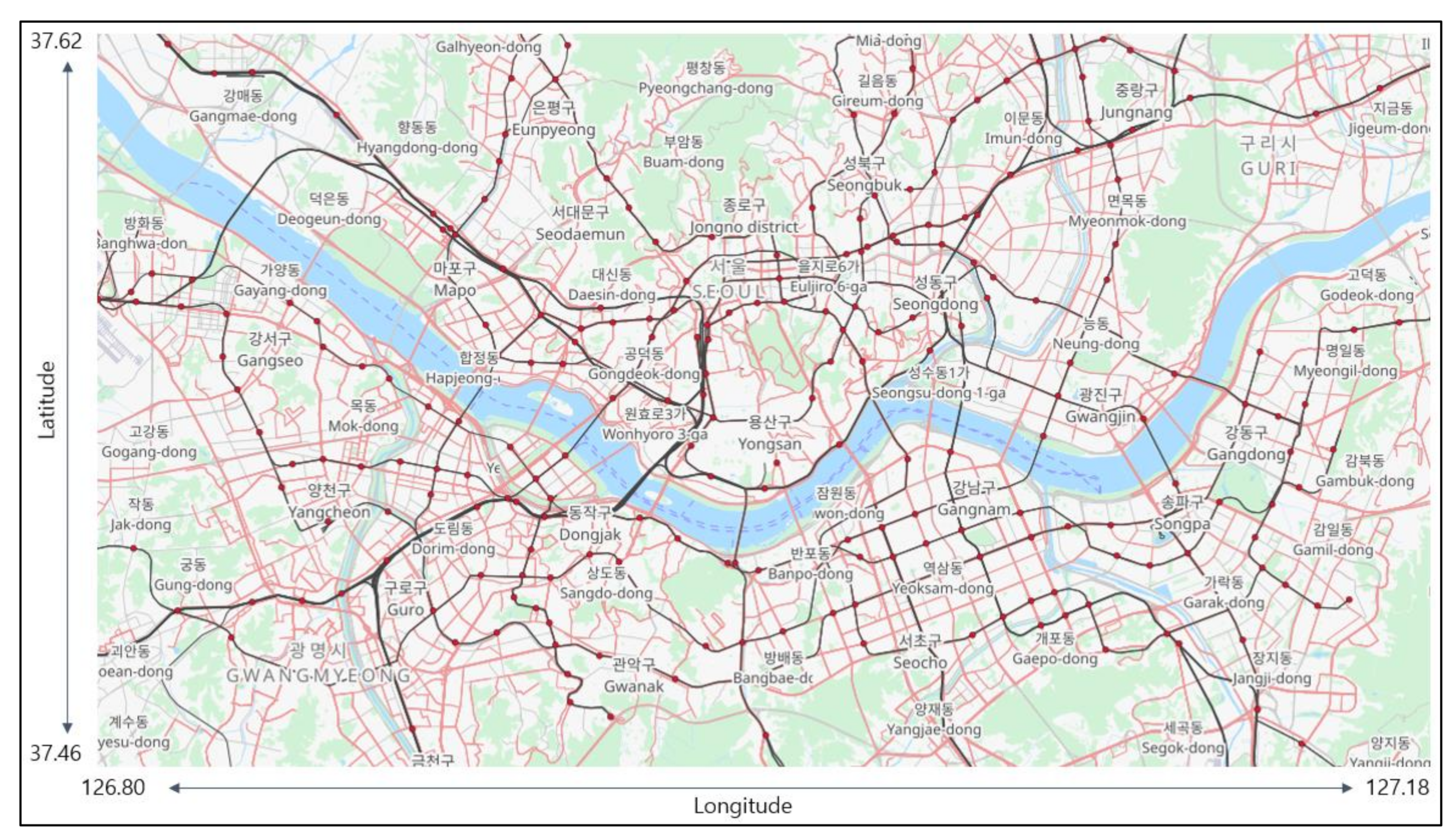
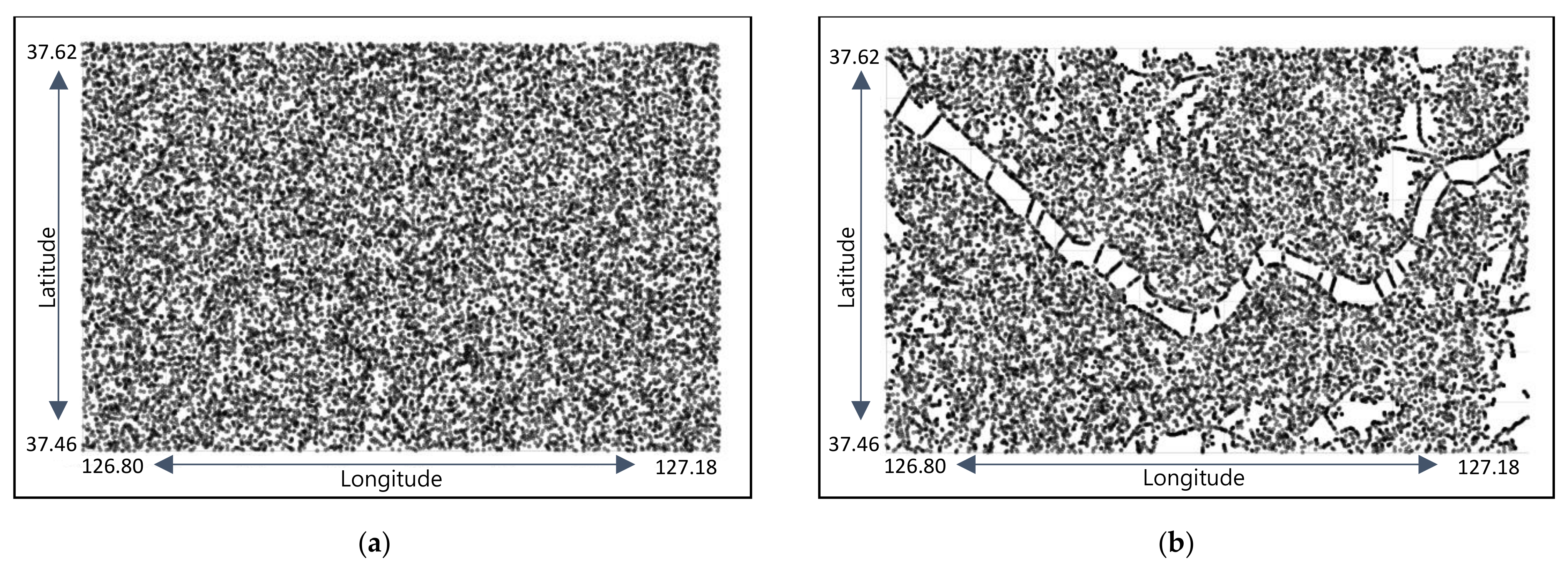
3.1. Training and Test Data

As shown in Figure 1, the latitude bound (37.46~37.62) and longitude bound (126.80~127.18) for the targeted area are set to include Seoul, the most populated city in South Korea. The size of the bounding box is approximately 17.5 by 33.5 km, which is rather large compared to previous studies on using ANN to estimate travel costs. Within the boundary, two geo-coordinates are randomly selected with uniform probability. The coordinates are then converted into the coordinates of the closest node in the road network, or the point of interest (POI). This conversion, illustrated in Figure 2, assures that paths should exist to connect the two locations in all samples. Note that forest (green) and water (blue) areas from Figure 1 are very well reflected in the converted points in Figure 2b. The shortest route with the travel distance and time values are provided with the help of GraphHopper routing engine [8] and map data of OpenStreetMap [9].

A total of 5 million samples are collected. 4.8 million samples were used for training the ANN model and the rest, 0.2 million samples, are used for testing the model. As shown in

Table 1. Examples of the collected samples for input and output values.

Sample Number	X (Input)				Y (Output)
	Longitude 1	Latitude 1	Longitude 2	Latitude 2	Distance (m)	Time (s)
1	126.9808	37.6141	127.1293	37.5760	17,511	1097
2	126.8230	37.5060	127.0829	37.5098	26,943	1400
3	127.0719	37.5136	126.9036	37.4888	17,235	1069
…	…	…	…	…	…	…

, each sample includes two geo-coordinates (the latitude and longitude of the origin and destination), and costs (the distance and time value of the travel).

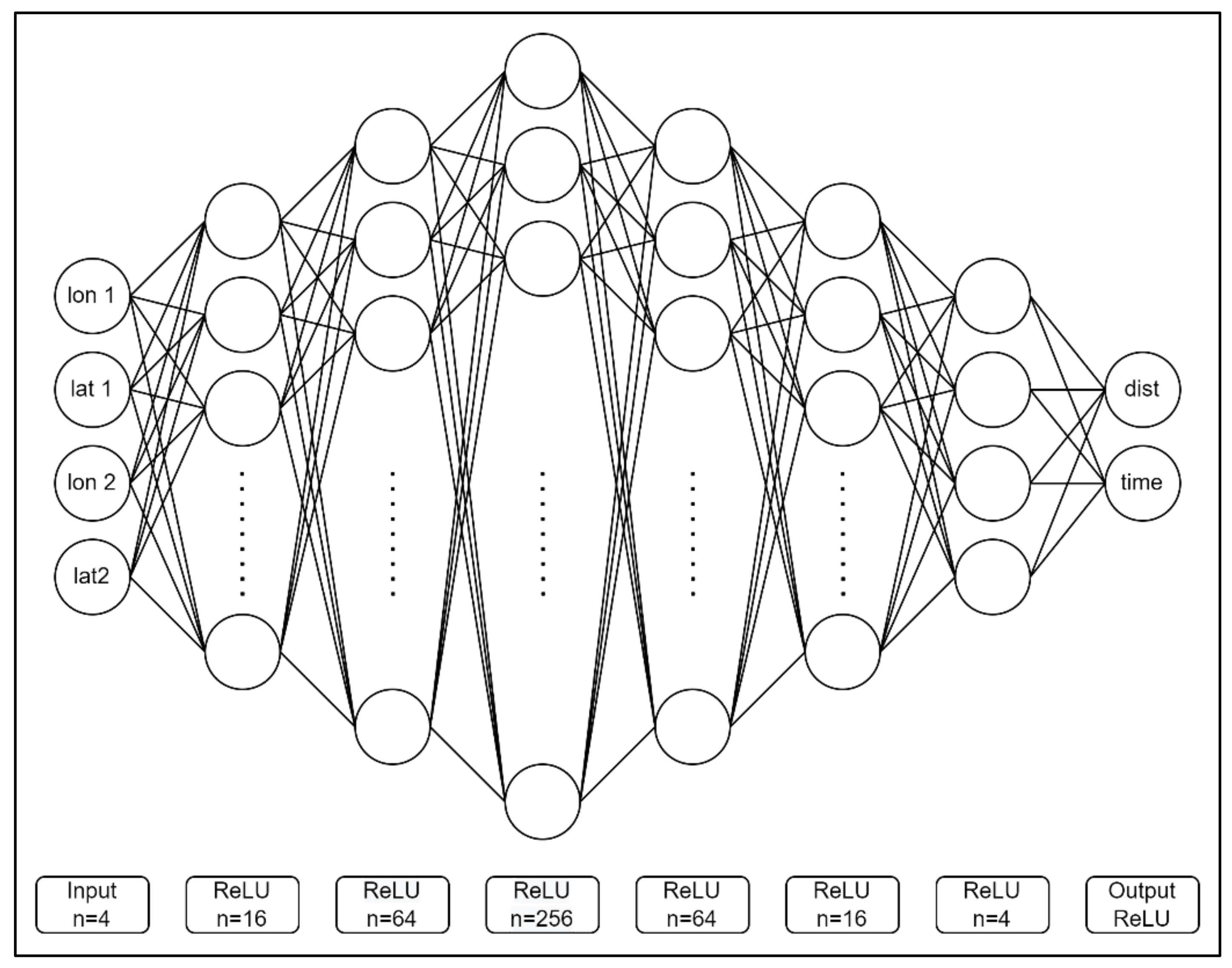
3.2. Model Construction and Train Parameters

As implied in Table 1, we construct an ANN model that receives coordinates of two POIs as input and draws travel distance and time values as output. Naturally, the model has four neurons in the input layer and two neurons in the output layer. As shown in Figure 3, the structure including input, hidden, and output layers is constructed as 4–16–64–256–64–16–4–2 neurons. All neurons in a layer are fully connected (linear) to the neurons in the next layer. Each layer includes the batch normalization [29] process that accelerates deep network training. For activation function, a rectified linear unit, usually abbreviated as ReLU, that is known to be effective in preserving information through multiple layers [30,31] is used.

The model is trained to minimize mean absolute percentage error (MAPE). The MAPE can be stated as provided below.

$$\mathrm{MAPE}=\frac{100\%}{n}{{\displaystyle \sum }}_{i=1}^n\left|\left(A_i-P_i\right)/A_i\right|$$

(1)

In the formula, $A_i$ is the actual value and $P_i$ is the predicted value of sample $i$. It is noted that the model has two output values to estimate, and the sum of MAPE for travel distance and for travel time is used in the training. In training the weights in the model, an adaptive moment estimation (Adam) optimizer that is known to be effective in learning complex systems [32] is used with a learning rate of 0.01. The size of the training batches is set to 8192 and the training data are shuffled when constructing the batches in every epoch. The model is trained over 1500 epochs. The training of the model took around 12 h using Intel i5-10600K CPU @ 4.10 GHz with 6 cores, and 16 GB of RAM.

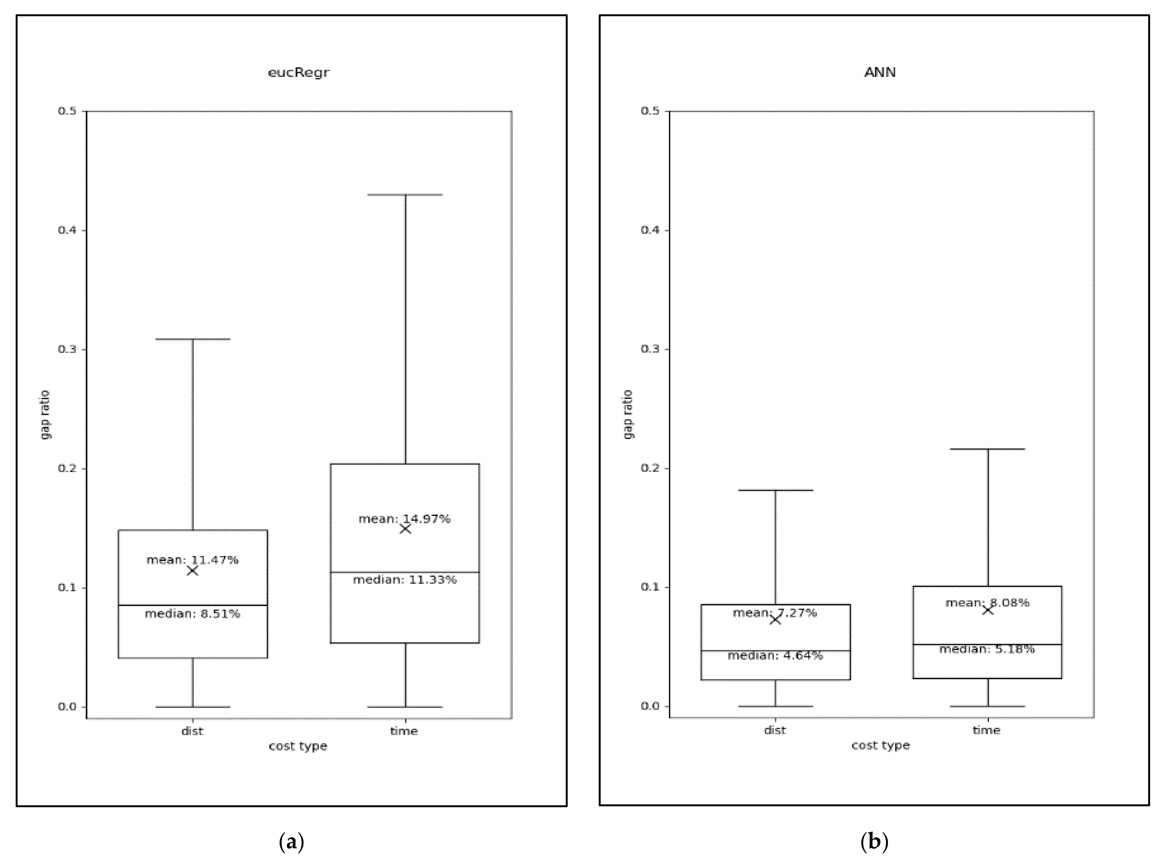
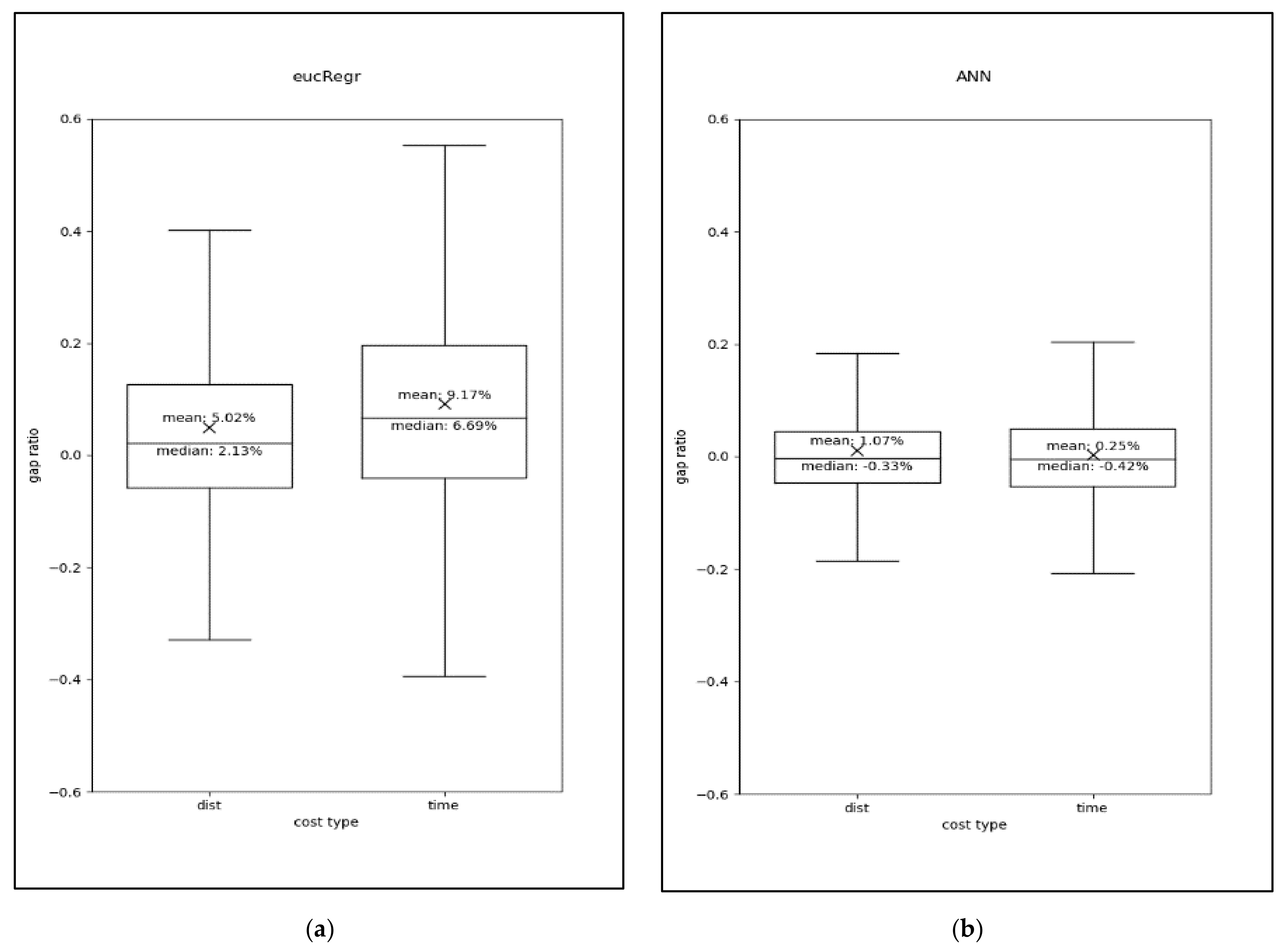
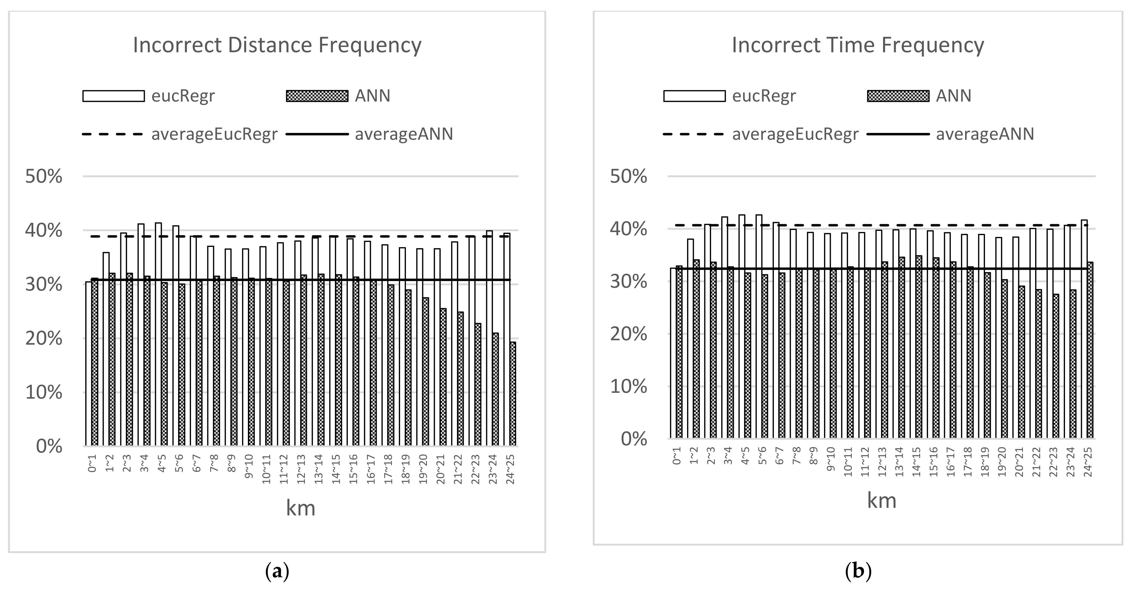
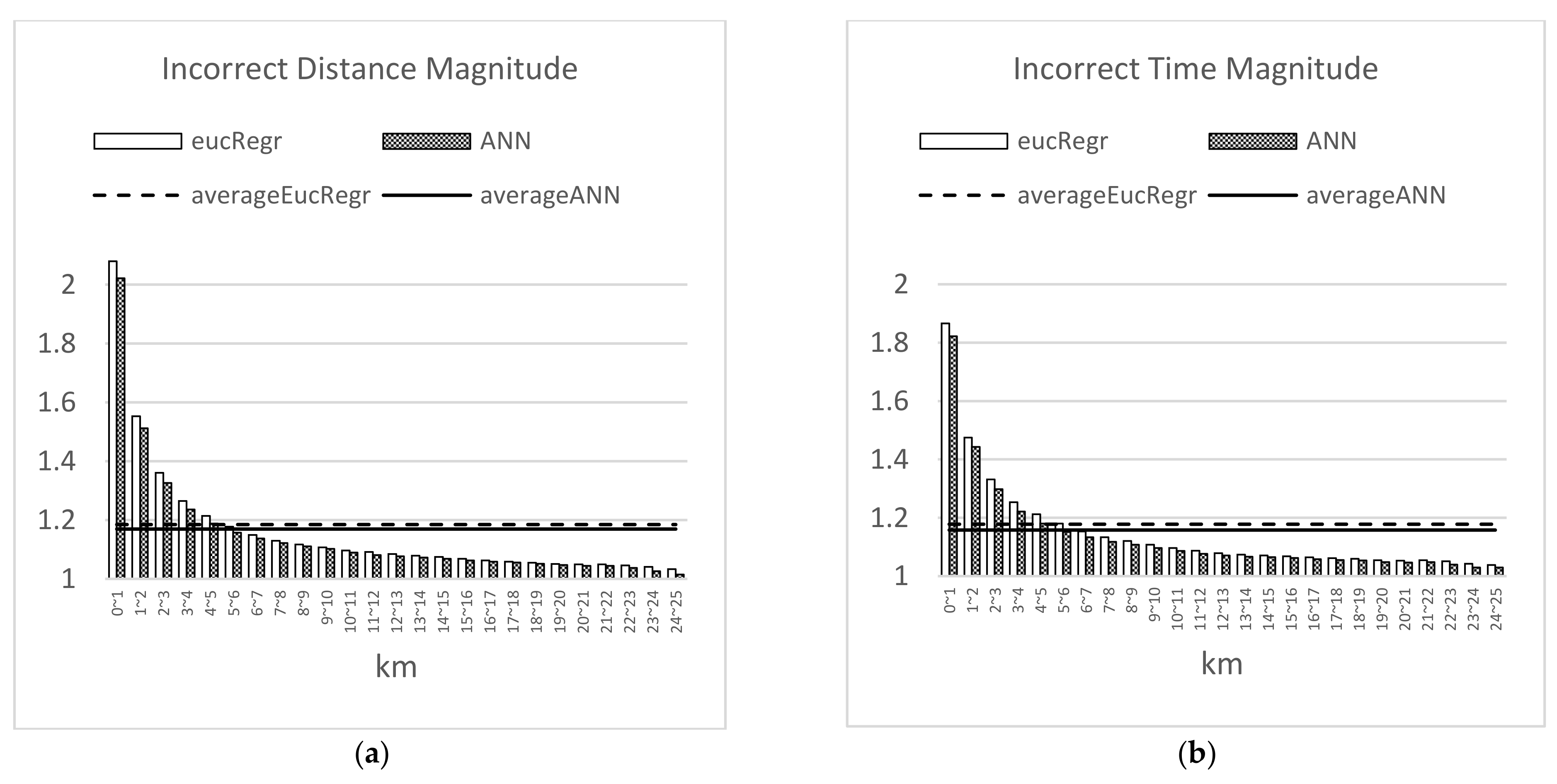
3.3. Estimation Performance of the Model

The trained ANN model is analyzed for its performance in comparison with a linear regression model. The linear regression method is used to find multiplication coefficients to the Euclidean distance ($\sqrt{{\left(lon1-lon2\right)}^2+{\left(lat1-lat2\right)}^2}$) that minimize the sum of squared errors in the test dataset. The coefficient for travel distance in meters, $b_m$, is found to be around 117,563, and the coefficient for travel time in seconds, $b_s$, is about 6589.

The ANN model and the regression model are compared in three different criteria. Since the objective of training ANN is to minimize MAPE, the first comparison criterion is on the percentage errors. Figure 4 compares absolute percentage errors of the two models, and Figure 5 compares the non-absolute percentage errors. Whether it is absolute or non-absolute, the ANN model exhibits better estimation quality. For the regression model’s result provided in Figure 4a, the MAPE measure for distance and time are 11.47% and 14.97% respectively, and the aggregated average of the two is 13.2%. Using the ANN model as provided in Figure 4b, the MAPE for distance and time are 7.27% and 8.08%. The aggregated average value is only 7.68%, which is 5.52% point lower than the regression model. The analysis of non-absolute percentage errors in Figure 5 also presents the superiority of the ANN model’s estimation.

The second comparison criterion is the closeness deceived by estimated cost, which was suggested in the work of Lee & Chae [6]. Suppose three POIs of nodes $i$, $j$ and $k$. The estimated cost from $i$ to $j$ and from $i$ to $k$ are measured and compared. The same comparison is subsequently carried out using actual road distance and road time. If the comparison using estimation and using actual cost selects different winners, the estimation is labelled inaccurate. How often (frequency) and how much (magnitude) the estimated cost chooses a false winner are both examined. The result on the frequency is provided in Figure 6. Figure 6a shows that using the regression model to decide which node is closer in distance measured has a 38.9% chance of giving wrong winners, while using the ANN estimation has a 30.8% chance. For the travel time measurement in Figure 6b, the regression model has a 40.7% chance, while the ANN model has a 32.4% chance of producing false winners. It is noted that the x-axes in the figures represent air distance ranges. The chances of false selection are calculated only when the two air distances from node $i$ to $j$ and from $i$ to $k$ are both in the same air distance range, which has intervals of one kilometer. When this condition is ignored, chances of deception are much lower, since they would include comparisons on some obviously large differences, e.g., air distance of 50 m and 2450 m. In ignorance of the condition, the regression model has a 6.5% chance, while the ANN model has a 5.7% chance of being wrong in selecting false winners using estimated travel distance. In estimation of travel time, the regression model is wrong 7.2% of the time, while the ANN model comes in lower at 6.4%.

The second criterion examines not only the frequency, as in Figure 6, but also the magnitude, as in Figure 7. It is more likely to be wrong when the two actual costs are similar and less likely when the two actual costs are largely different. When the closeness measurement is wrong, the magnitude is calculated as the cost from $i$ to $j$ divided by the cost from $i$ to $k$, with the denominator being the smaller value. Figure 7a shows that when the wrong winner is chosen by distance estimations, the average difference magnitude of the two actual values is 1.185 times. On the other hand, the ANN model has the magnitude of 1.169. For time estimations as shown in Figure 7b, the average difference magnitude of being wrong in the regression model is 1.178, while it is 1.158 in the ANN model. In every aspect of performance evaluation in the second criterion (whether on frequency or on magnitude, and on any range of air distance intervals), the ANN model outperforms the regression model.

The third comparison criterion is the correctness rate of selecting a specified number of closest neighbors. Arnold et al. [33] analyzed collections of optimal VRP solutions and reported that the nodes were connected to the 20 closest neighbors 95% of the times, and to the 50 closest neighbors 99% of the times. The study implies that solutions of good quality can still be obtained when edges to only some closest neighbors are available. This selective strategy has been an efficient way of solving large-sized VRP instances. The third criterion is to see how well the estimated distance or time can select a specified number of closest neighbors correctly. Figure 8 summarizes the result of correctness rate when closest neighbors in distance are estimated using the regression model and the ANN model. The x-axes in the figures represent the targeted closest neighbor counts. In Figure 8a, for instance, when ten neighbors are chosen using the Euclidean distance, 77% of them are correct on average. Using the ANN model, on the other hand, the correctness is about 80.1%. The correctness increases as the targeted closest neighbor count increases. Figure 8a–c are different in terms of the total number of nodes in the analysis: 100, 500, and 1000. When a larger number of nodes are drawn within the specified range of longitude and latitude, the distance between the nodes become denser. When nodes are densely populated, it is harder to determine the closest neighbors correctly as the tendency shown in the three figures. For example, when ten closest neighbors are determined from a total of 100 nodes using the ANN model, the correctness is around 80.1% as in Figure 8a, while it is 66.1% from a total of 1000 nodes as in Figure 8c. Figure 9 presents results of the same analysis as Figure 8, but with the time estimations. In every aspect of the performance evaluation in Figure 8 and Figure 9, for different measure of distance and time, for different number of nodes to choose from, and for different targeted closest neighbor counts, the ANN model surpasses the quality of using the Euclidean distance.

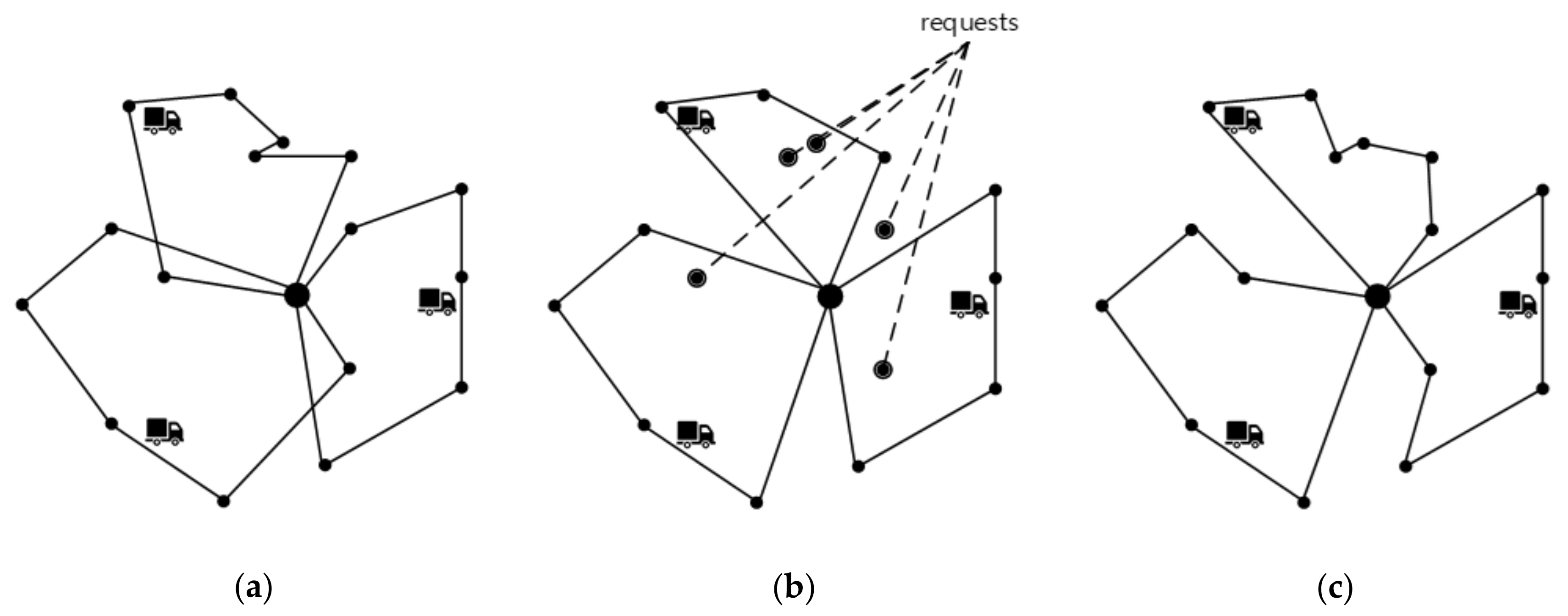
4. Potential Application in Vehicle Routing Problems

In the previous section, the performance of the ANN model for distance and time estimation is confirmed to be superior to the simple regression model on Euclidean distance. In general, better VRP solution quality is expected with a more precise cost matrix. In this study, the utility of the ANN model is further examined for various implementation scenarios on the VRP to see if it is as beneficial as expected.

4.1. Scenario Design

The scenarios are constructed to verify that using the ANN model for cost matrix creation instead of Euclidean distance is favorable. The implementation scenarios of the ANN on VRPs are designed as provided in

Table 2. Implementations scenarios of the ANN on VRP.

Scenarios		Matrix Type	Cost Type	Details
S0 (Base)		Full OSM matrix for VRP	Distance	-
			Time
S1	S1-1	Full EucDist matrix for VRP	Distance
			Time
	S1-2	Full ANN matrix for VRP	Distance
			Time
S2	S2-1	Full EucDist matrix for VRP and partial OSM matrices for TSPs	Distance	After running VRP, run TSP for each vehicle
			Time
	S2-2	Full ANN Matrix for VRP and partial OSM matrices for TSPs	Distance
			Time
S3	S3-0	Partial OSM matrix for VRP	Distance	50 closest neighbors based on OSM
			Time
	S3-1	Partial OSM matrix for VRP	Distance	50 closest neighbors based on EucDist
			Time
	S3-2	Partial OSM matrix for VRP	Distance	50 closest neighbors based on ANN
			Time

.

The ‘S0’ scenario is the base scenario, where OpenStreetMap (OSM) matrix is used to solve the VRP. Here, the OSM matrix refers to the road distance or road time matrix obtained using the GraphHopper routing engine [8]. In the experiment, the base scenario is assumed to produce the base quality of the VRP solution, and the qualities of the VRP in other scenarios are compared to the base scenario. The solution quality can be defined as the sum of vehicle routes’ travel cost, which is used as the objective function value (OFV) in most VRP research. This research also examines another aspect of quality, the response time that includes the time for matrix creation and problem solving. Since response time for the solution matters in real operations, it is reasonable to consider the cost matrix creation time for quality.

The ‘S1’ scenarios include the use of Euclidean distance (EucDist) and the ANN model for cost matrix creation. It is noted that scenario names ending with ‘-1’ imply the use of Euclidean distance matrix and the ones ending with ‘-2’ imply the use of the ANN model. The ‘S1-1’ scenario makes use of the Euclidean distance matrix for solving the VRP. After the problem is solved, the solution’s OFV is recalculated by using the actual road distance or road time, with the OSM matrix. Note the vehicle assignments and visiting sequence of nodes in the solution are intact in the recalculation process. The recalculation is only to see how suboptimal the solution is from the base scenario. The ‘S1-2’ scenario follows the same process, but with the only difference in matrix creation method.

The ‘S2’ scenarios aim to improve the solution quality of ‘S1’ with some partial OSM matrices. That is, after solving the VRP with estimated costs, each vehicle’s visiting sequence is reconstructed by solving TSP with the actual OSM cost for each vehicle. The full matrix for the VRP being the $\left(N\times N\right)$ matrix, where $N$ is the number of nodes, partial matrices are smaller sets of elements from the full matrix. For instance, if the problem has ten vehicles and each vehicle is assigned ten visiting locations, then the required partial matrices for solving TSPs are $\left(10\times 10\times 10\right)$. The size of the partial matrices in the example is ten times smaller than the full $\left(100\times 100\right)$ matrix.

The ‘S3’ scenarios are also designed to use only some portion of the OSM matrix. For each visiting node, the 50 closest nodes are determined. In the determination of the closest nodes, scenario ‘3-0’, ‘3-1’, and ‘3-2’ use OSM costs, Euclidean distance, and the ANN model’s estimation, respectively. Then, the cost matrix size of $\left(N\times 50\right)$ is created to solve the VRP. In scenario ‘3-0’, the OSM costs are already obtained in the closest node selection process, and they are ready to be used. In the other two scenarios, the OSM costs are requested after the selection process. It is noted that in a strict sense, the size of the cost matrix is $50\left(N-1\right)+2\left(N-1\right)$, since costs for all edges connecting to the depot are fully required. However, this paper simplifies the notation as $\left(N\times 50\right)$.

4.2. Instance Creation and Solution Method

The experimental instances are created to test the implementation scenarios. For any instance, the number of vehicles is fixed to ten. Within the territorial boundaries described in Section 3.1, customer nodes are randomly selected with uniform distribution. The number of nodes to be created for the problem instances are set to be 100, 500, and 1000. For each problem size, 300 replications of instances are created. Each replication includes problem solving of eight scenarios, from ‘S0’ to ‘S3-2’. Each scenario includes two cost matrix types (distance and time), and two parameter settings for the problem-solving algorithm (short search and long search). In total, the problems are solved for 28,800 (3 different problem sizes by 300 replications by 8 scenarios by 2 matrix types by 2 parameter settings) times.

The large neighborhood search (LNS) algorithm [34] is used for solving VRP and TSP in the experiments. The LNS algorithm explores the current solution’s neighborhoods by removing a large portion of customer nodes from the solution and re-inserting these nodes. Figure 10a shows an initial suboptimal solution of the given VRP instance with the depot in the centre and three vehicle routes. In Figure 10b, customers have been removed from the routes. The neighborhood contains all solutions that can be created by reinserting the customers into the routes. Figure 10c represents such a solution. To be able to provide solutions that are close to the optimal solutions, an improved version of LNS from the work of Lee [35] is employed. In that study, the simulated annealing (SA) algorithm [36] is used as a meta-heuristic algorithm. For each annealing temperature in the cooling schedule, a specified number of LNS iteration is carried out. The number of iterations is the parameter setting to decide if the solution search is short or long. For the short and the long search, the iteration parameter is set to 1000 and 5000, respectively.

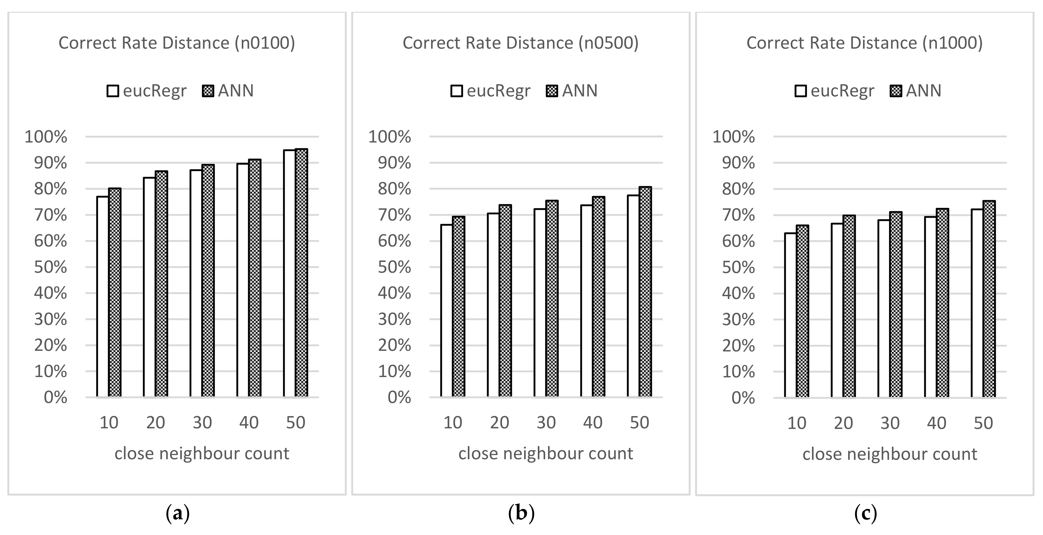
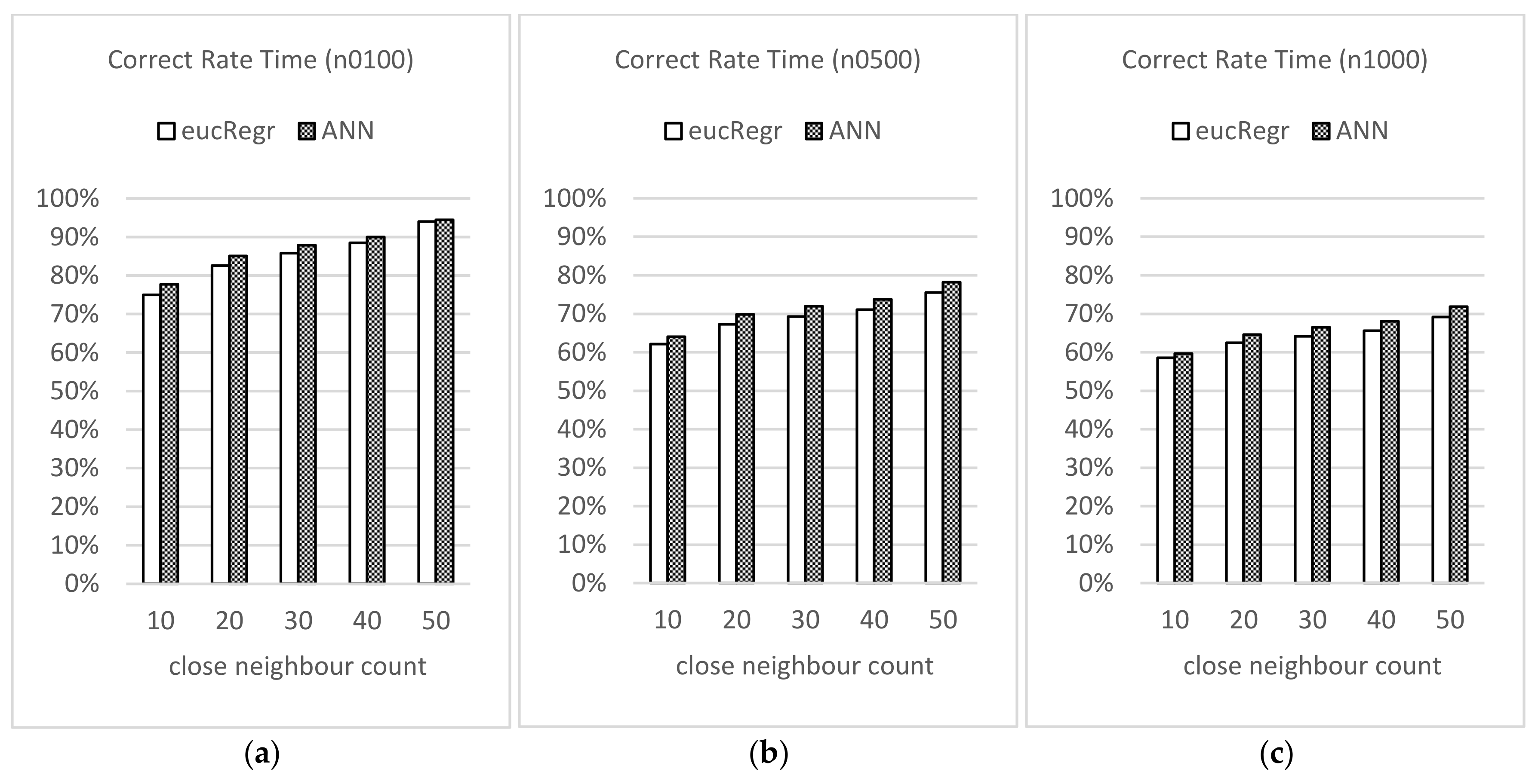
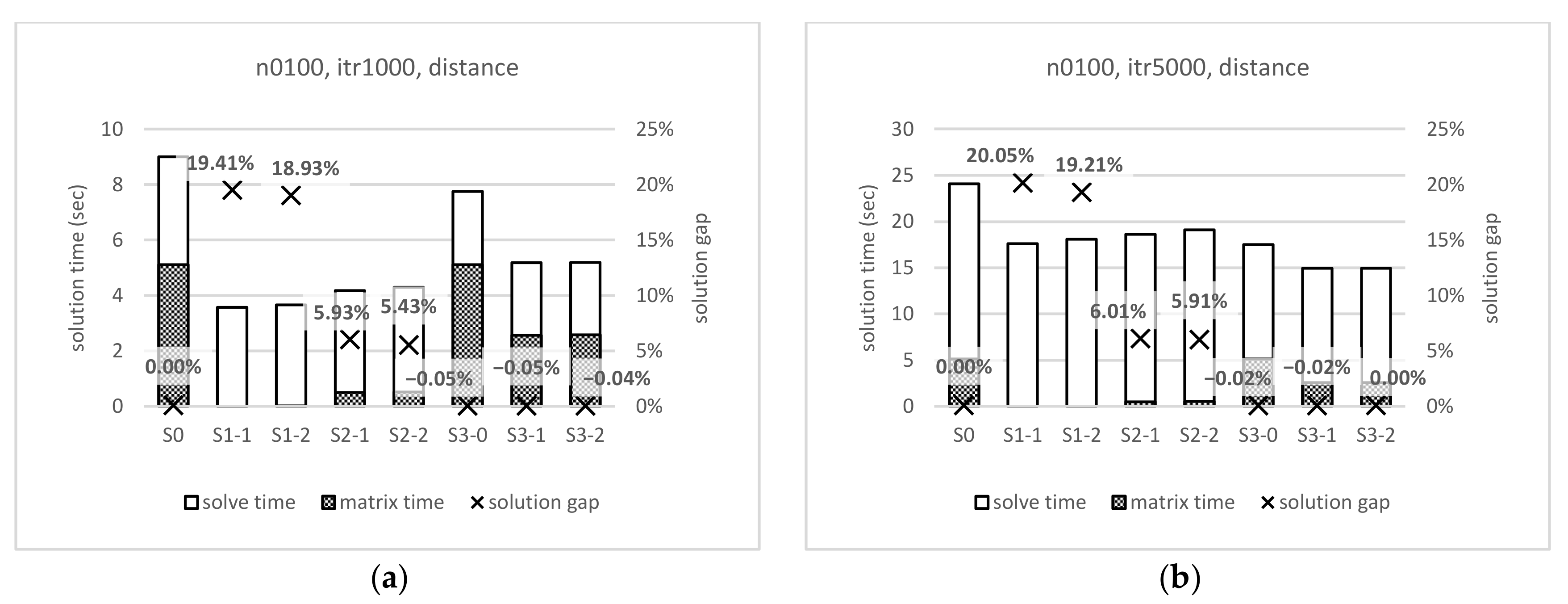
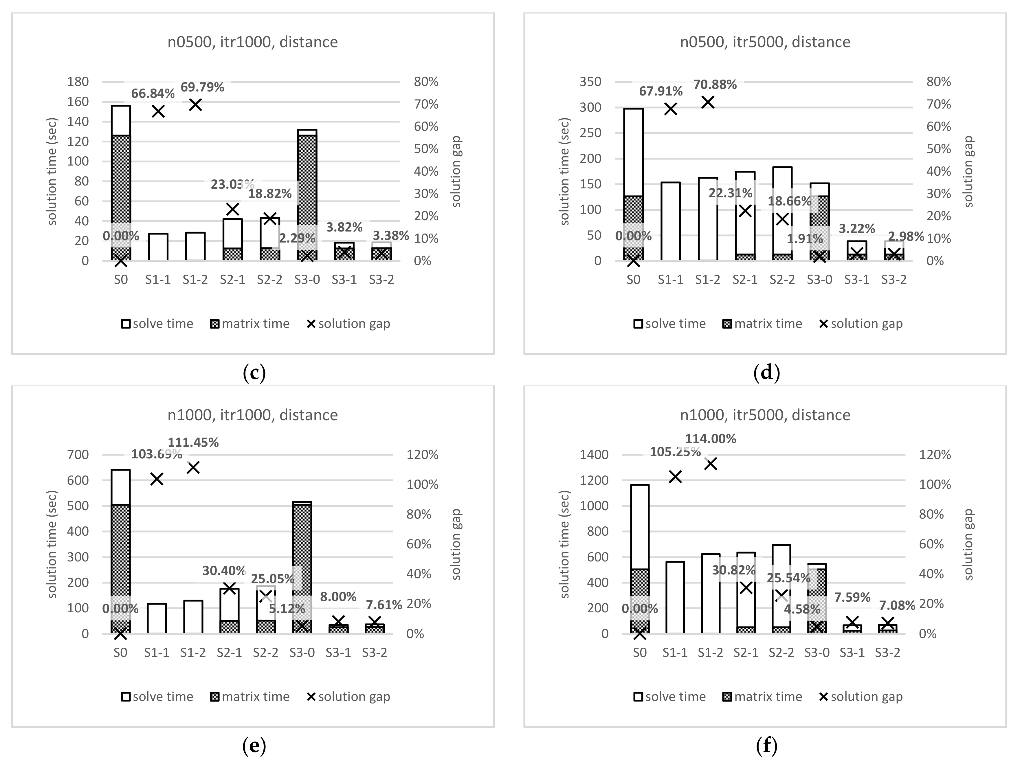
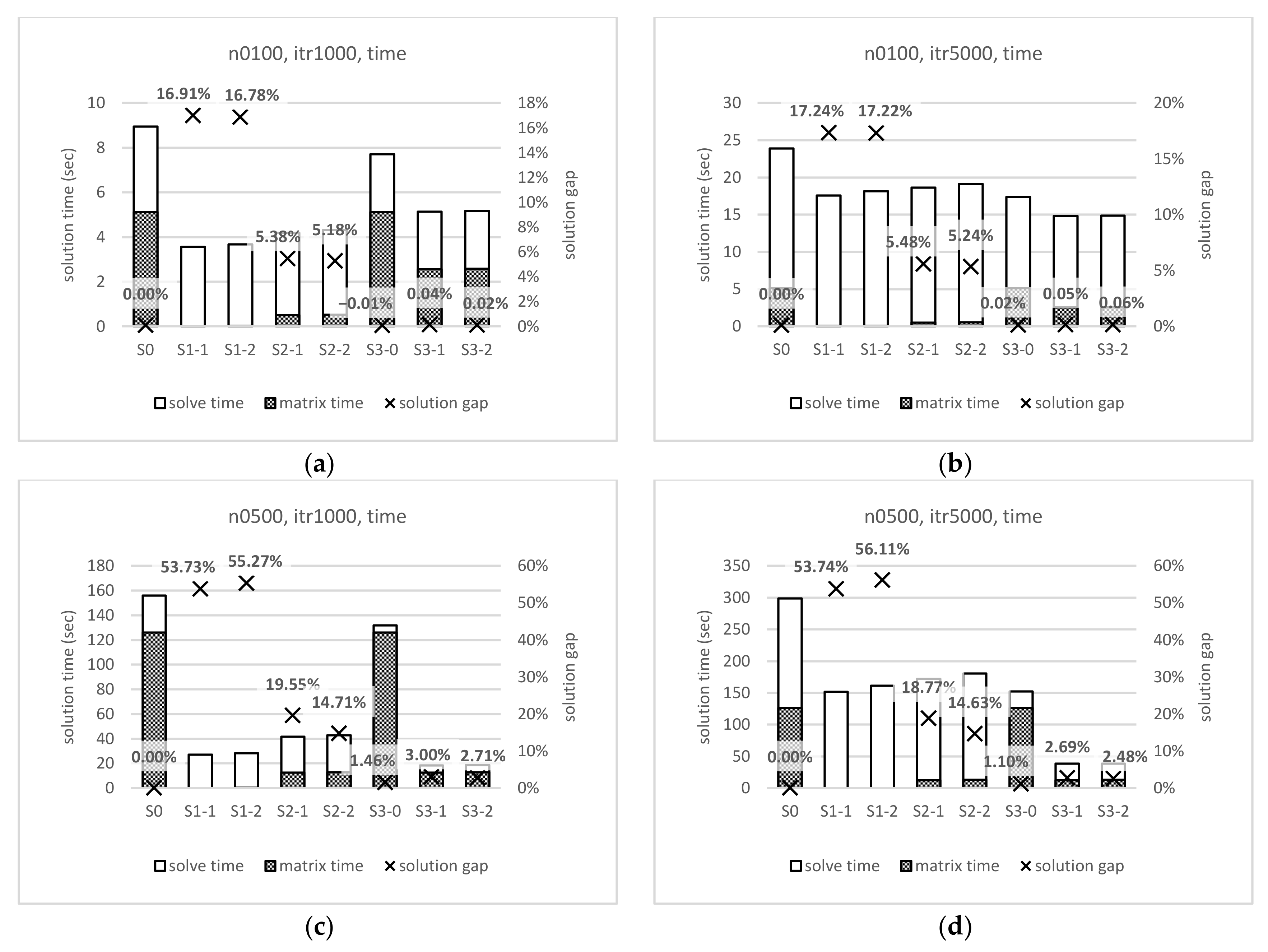
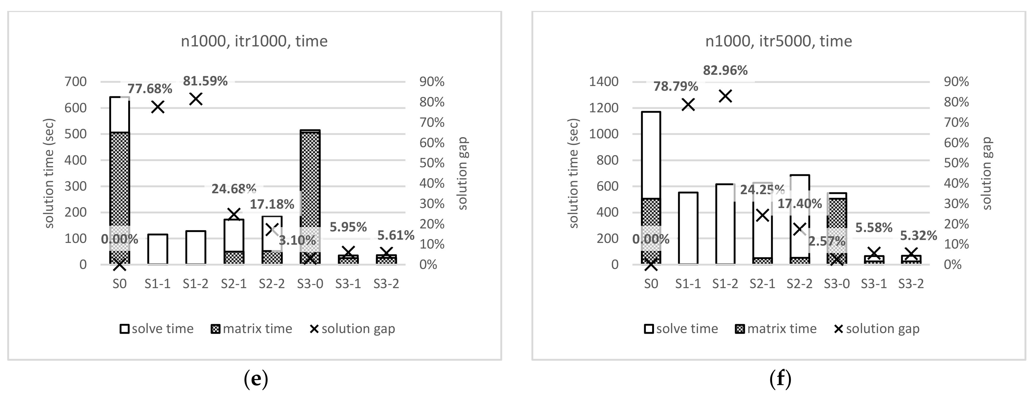
4.3. Experimental Results

An Intel i5-10600K CPU @ 4.10 GHz and 16 GB of RAM are used for the experiments. Figure 11 and Figure 12 summarize the experimental results of various implementation scenarios provided in Table 2. The two figures are separated by the type of the cost matrix (distance and time). Each of the two figures contains six graphs that are distinguished by the size of the problem and the parameter settings of LNS iterations. The scenario names are displayed in the x-axes. Note that there are two y-axes in each graph. The response time is measured at the left y-axis with bar graphs. Each bar consists of problem-solving time (non-shaded) and matrix creation time (shaded). The right y-axis measures the solution gap (%) from the base scenario with ‘x’ marks. Since the solution gap is the difference between the average OFV for a scenario and the average OFV for the base scenario, divided by the average OFV for the base scenario, the solution gap for the base scenario is marked as 0%. The following are the major findings from the experiments.

First, employing the ANN model for matrix creation, instead of Euclidean distance, is verified to be beneficial in VRP as expected. For ‘S1’ scenarios, the advantage of the ANN model is not certain. Rather, the use of Euclidean distance seems to provide better solution quality in many cases. However, in ‘S2’ and ‘S3’ scenarios, using the ANN model surely outperformed the Euclidean distance. That is, ‘S2-2’ produces better solutions than ‘S2-1’, and similarly for ‘S3-2’ and ‘S3-1’. To prove the effectiveness of the ANN model, the solution gaps of ‘S2-1’ and ‘S2-2’ are compared using the t-test as shown in

Table 3. t-test to compare the implementation scenario ‘S2-1’ and ‘S2-2’.

Cost Type	Problem Size	LNS Iteration	Scenario	Mean Gap from S0	Variance	Degree of Freedom	t-Statistics	$\mathit{p} (\mathbf{T} \le$ t)
Distance	100	1000	S2-1	0.059340	0.000447	593	3.032024	0.002535 (<0.01)
			S2-2	0.054336	0.000370
		5000	S2-1	0.060147	0.000366	595	0.687932	0.491764 (>0.05)
			S2-2	0.059109	0.000316
	500	1000	S2-1	0.230325	0.001727	575	13.60022	1.01 × 10−36 (<0.001)
			S2-2	0.188196	0.001151
		5000	S2-1	0.223133	0.001536	594	11.89121	2.12 × 10−29 (<0.001)
			S2-2	0.186558	0.001302
	1000	1000	S2-1	0.303998	0.003369	544	12.95487	1.21 × 10−33 (<0.001)
			S2-2	0.250463	0.001754
		5000	S2-1	0.308150	0.003582	543	12.40323	2.8 × 10−31 (<0.001)
			S2-2	0.255393	0.001846
Time	100	1000	S2-1	0.053796	0.000306	598	1.411387	0.158651 (>0.05)
			S2-2	0.051796	0.000296
		5000	S2-1	0.054809	0.000275	597	1.81339	0.070274 (>0.05)
			S2-2	0.052409	0.000251
	500	1000	S2-1	0.195454	0.001088	582	19.36356	7.51 × 10−65 (<0.001)
			S2-2	0.147109	0.000782
		5000	S2-1	0.187688	0.001239	535	16.68161	1.3 × 10−50 (<0.001)
			S2-2	0.146321	0.000606
	1000	1000	S2-1	0.246780	0.002444	460	23.11096	5.35 × 10−79 (<0.001)
			S2-2	0.171819	0.000712
		5000	S2-1	0.242476	0.002457	454	21.17282	1.03 × 10−69 (<0.001)
			S2-2	0.173965	0.000685

. The t-test for the ‘S3-1’ and ‘S3-2’ comparison is also provided in

Table 4. t-test to compare the implementation scenario ‘S3-1’ and ‘S3-2’.

Cost Type	Problem Size	LNS Iteration	Scenario	Mean Gap from S0	Variance	Degree of Freedom	t-Statistics	$\mathit{p} (\mathbf{T} \le$ t)
Distance	100	1000	S3-1	−0.00051	5.43 × 10−5	593	−0.27505	0.78337 (>0.05)
			S3-2	−0.00035	4.52 × 10−5
		5000	S3-1	−0.00020	1.64 × 10−5	597	−0.70038	0.483964 (>0.05)
			S3-2	2.61 × 10−5	1.50 × 10−5
	500	1000	S3-1	0.038191	0.000367	590	2.96851	0.003114 (<0.01)
			S3-2	0.033792	0.000292
		5000	S3-1	0.032218	0.000228	596	1.988923	0.047166 (<0.05)
			S3-2	0.029834	0.000203
	1000	1000	S3-1	0.080004	0.000563	597	2.073294	0.038573 (<0.05)
			S3-2	0.076061	0.000522
		5000	S3-1	0.075898	0.000481	594	2.977116	0.003028 (<0.01)
			S3-2	0.070769	0.000409
Time	100	1000	S3-1	0.000427	3.21 × 10−5	598	0.579254	0.562636 (>0.05)
			S3-2	0.000161	3.12 × 10−5
		5000	S3-1	0.000478	1.03 × 10−5	597	−0.31144	0.755578 (>0.05)
			S3-2	0.000561	1.11 × 10−5
	500	1000	S3-1	0.030004	0.000177	597	2.757916	0.005995 (<0.01)
			S3-2	0.027065	0.000164
		5000	S3-1	0.026874	0.000128	598	2.263893	0.023938 (<0.05)
			S3-2	0.024801	0.000123
	1000	1000	S3-1	0.059465	0.000304	596	2.464255	0.014011 (<0.05)
			S3-2	0.056052	0.000271
		5000	S3-1	0.055786	0.000218	598	2.154696	0.031584 (<0.05)
			S3-2	0.053207	0.000212

. The mean gap from ‘S0’ in the tables is calculated as the sum of OFV from a specific scenario minus the sum of OFV from ‘S0’, divided by the number of replications.

The results in the tables verify that the average solution gap differences are statistically significant, particularly in problem sizes of 500 and 1000. In the small size of 100, the results of the t-test do not verify the significance of the differences. This can be explained by the fact that the LNS algorithm finds solutions that are optimal, or almost optimal, most of the time in small sized problems, and the differences are too small to be verified as statistically significant. It is noted that the average difference is much more significant in Table 3 (‘S2-1’ to ‘S2-2’ comparison) than in Table 4 (‘S3-1’ to ‘S3-2’ comparison).

Second, the solution OFV gaps of using time matrices are smaller than using distance matrices for both Euclidean estimation and the ANN model estimation. That is, the solution gaps marked in Figure 12 (time) are lower than the values marked in Figure 11 (distance), given the problem size and the iteration limits. For example, in cases of problem size 1000 and LNS iteration 5000, which are the (f) figures, the solution gaps of ‘S2-1’ are 30.82% for distance and 24.25% for time with Euclidean estimations. When the ANN model is used for the costs (‘S2-2’), it showed a 25.54% solution gap for distance and 17.40% for time. This trend is commonly observed when Figure 11 and Figure 12 are compared piece by piece. This is opposite to the original expectation, since the performance evaluation of Euclidean and ANN estimations conducted in Section 3.3 has shown that the estimations better predict distance than time in most criteria. Revisiting Figure 7, the only performance measure favourable to time over distance is the deception magnitude. The average difference magnitude values are favourable to time estimations more than distance, but the gap is not noticeable much in the interval of {0~25} km. However, for the interval of {0~1} km, where most optimal VRP solutions are supposed to be susceptible, the value differences are more prominent. In Euclidean estimation, the magnitude is 2.08 for distance and 1.87 for time, while it is 2.02 for distance and 1.82 for time in the ANN estimation. An emphasis should be put on the deception magnitude criterion when the estimations are meant to be used in solving VRPs.

Third, there exist promising implementation strategies for the ANN model, considering the solution gap of OFV and response time. As underlined in this research, response time for the VRP solution matters in the operational level. It is shown in Figure 11 and Figure 12 that the matrix creation time accounts for a large portion of the response time when road distance or road time are to be used with the help of a routing engine. For more detailed analysis, the average matrix creation time and problem-solving time presented in Figure 11 and Figure 12 are restated with more precise numbers in

Table 5. Average matrix creation time and problem-solving time from experimental results.

Time	Matrix Size	$\mathbf{Problem} \mathbf{Size} \left(\mathit{N}\right)$	OSM	EucDist	ANN
Matrix creation	$\left(N\times N\right)$	100	5.12 s	<0.01 s	<0.01 s
		500	126.12 s
		1000	505.13 s
	$\left(10\times n\times n\right)$	100	0.52 s
		500	12.79 s
		1000	51.18 s
	$\left(N\times 50\right)$	100	2.57 s
		500	12.80 s
		1000	25.9 s
Problem-solving	$\left(N\times N\right)$	100		2.72 s
		500		28.46 s
		1000		127.51 s
	$\left(10\times n\times n\right)$	100		3.69 s
		500		29.81 s
		1000		130.17 s
	$\left(N\times 50\right)$	100		2.62 s
		500		5.70 s
		1000		9.82 s

. In the table, the matrix size (N × N) refers to the full cost matrix, (10 × n × n) refers to the partial cost matrix required for TSP for each vehicle of ten, and (N × 50) refers to the partial cost matrix for 50 closest nodes.

A huge matrix creation time gap between using a routing engine and using estimations is noted. For $\left(N\times N\right)$ OSM cost matrices, the average creation time is 5.12 s with 100 nodes, 126.12 s with 500 nodes, and 505.13 s with 1000 nodes. It is clear from the results that matrix creation consumes much more time than problem-solving, from double to almost quadruple in some cases. Moreover, the matrix creation time can be even greater with more accurate commercial routing engine APIs. On the other hand, the creation of the Euclidean distance matrix only takes an instant. Likewise, the ANN model, which has already been trained in advance, takes only a split second given the simple structure described in Section 3.2. Since the problem-solving is ignorant of how the cost matrices are created, problem-solving times do not differ by the sources (OSM, EucDist, and ANN), as expressed in the table. Considering the small OFV gaps in most cases and the dramatic decrease in the response times, scenario ‘S3-1’ with Euclidean estimation and ‘S3-2’ with the ANN model estimation are both acceptable implementation scenarios. However, it is identified that the ANN model, provided with enough training time in advance, estimates cost better, while having almost the same matrix creation time.

5. Conclusions

The use of straight-line distance, or Euclidean distance, heavily distorts the actual travel cost, while the use of accurate routing engines requires a lengthy response time or high usage fee. Alternative methods of obtaining better estimated cost matrices without adding too much time or fee are worth consideration in VRP application.

This study constructed and trained an ANN model for estimating the travel cost between two geo-coordinates within a bounded territory. The ANN model receives four input values, which are the latitudes and longitudes for the two coordinates, and produces two output values, the travel distance and time. The trained ANN model is compared to the Euclidean estimation for performance evaluation using multiple criteria, including MAPE, frequency and magnitude of closeness deception, and the ability to identify some number of closest neighbors. In every aspect of the evaluation, the ANN model is verified to outperform the Euclidean estimation.

The ANN model is further examined for potential implementation strategies in VRP. Scenarios are constructed to compare the utility of the ANN estimations when full or partial cost matrices are used. As expected from the estimation performance evaluations, using cost matrices from ANN estimation, instead of Euclidean estimation, results in smaller OFV gap in VRP solutions. The differences in OFV gaps of the two estimation methods are verified to be statistically significant. It is noted that given the training time in advance, the matrix creation time for the ANN model is almost the same as the Euclidean distance calculation.

Suggestions are made from the experimental results. When the VRP solution quality is comprised of both OFV gap and response time, there exist promising VRP implementation scenarios where the ANN estimations are used for cost matrix creation. Euclidean estimations are also fast, but the ANN estimations produce better results with almost no increase in matrix creation time. It is noted that in most performance evaluation criteria, distance estimations were better than time estimations. The only measure in which the distance estimations were poor in performance was the deception magnitude, but it did have a major impact on the VRP solutions. The OFV gaps of using estimated distance matrices turned out to be higher than using estimated time matrices. Accordingly, the performance criteria of deception magnitude should be paid more attention in future research.

The ANN model in this study is not perfect. By the innate nature of machine learning, the performance of the model is dependent on the training data. The estimations are only valid within the specified bounding box, and any changes in the road network cannot be immediately accommodated into the model. Moreover, the training data did not consider different traffic conditions at different times of the day. Future research should be directed by the model’s limitations. Research on ways to reflect changes in the network or the traffic conditions are called for. Regarding traffic conditions, traffic speed prediction methods [37,38] can be consulted in future research. This research verified that a simple ANN model for cost matrix creation is worth implementing in VRPs. A simple structure was employed considering the large size of targeted territory. However, ANN models with higher accuracy are expected to bring even more benefit, and thus, improvements on the model, such as different loss functions or different structures (deeper or larger), need to be tested in future research.

References

1. Toth, P.; Vigo, D. The Vehicle Routing Problem; Society for Industrial and Applied Mathematics: Philadelphia, PA, USA, 2002; ISBN 0-89871-498-2. [Google Scholar]
2. Laporte, G.; Nobert, Y. Exact Algorithms for the Vehicle Routing Problem. North-Holl. Math. Stud. 1987, 132, 147–184. [Google Scholar] [CrossRef]
3. Gower, J.C. Properties of Euclidean and non-Euclidean distance. Linear Algebra Appl. 1985, 67, 81–97. [Google Scholar] [CrossRef]
4. Smet, G. De OptaPlanner-Vehicle Routing with Real Road Distances. Available online: https://www.optaplanner.org/blog/2014/09/02/VehicleRoutingWithRealRoadDistances.html (accessed on 9 June 2022).
5. Boyacı, B.; Dang, T.H.; Letchford, A.N. Vehicle routing on road networks: How good is Euclidean approximation? Comput. Oper. Res. 2021, 129, 105197. [Google Scholar] [CrossRef]
6. Lee, K.; Chae, J. A proposal and analysis of new realistic sets of benchmark instances for vehicle routing problems with asymmetric costs. Appl. Sci. 2021, 11, 4790. [Google Scholar] [CrossRef]
7. Google Maps Distance Matrix API. Available online: https://developers.google.com/maps/documentation/distance-matrix/overview (accessed on 9 June 2022).
8. GraphHopper. GraphHopper Routing Engine. Available online: https://github.com/graphhopper (accessed on 9 June 2022).
9. OpenStreetMap. Setting Up a Local Copy of the OpenStreetMap Database. Available online: https://wiki.openstreetmap.org/wiki/Setting_up_a_local_copy_of_the_OpenStreetMap_database,_kept_up_to_date_with_minutely_diffs (accessed on 9 June 2022).
10. Ballou, R.H.; Rahardja, H.; Sakai, N. Selected country circuity factors for road travel distance estimation. Transp. Res. Part A Policy Pract. 2002, 36, 843–848. [Google Scholar] [CrossRef]
11. Gonçalves, D.N.S.; Gonçalves, C.D.M.; De Assis, T.F.; Silva, M.A. Da Analysis of the difference between the euclidean distance and the actual road distance in Brazil. Transp. Res. Procedia 2014, 3, 876–885. [Google Scholar] [CrossRef]
12. Phibbs, C.S.; Luft, H.S. Correlation of the travel time on roads versus stright line distance. Med. Care Res. Rev. 1995, 52, 532–542. [Google Scholar] [CrossRef]
13. SK Telecom TMAP API. Available online: https://openapi.sk.com/API/detail?svcSeq=4#pay (accessed on 11 June 2020).
14. Naver Cloud Plaform Maps Application Services-NAVER Cloud Platform. Available online: https://www.fin-ncloud.com/product/applicationService/maps (accessed on 11 June 2022).
15. OSRM. Open Source Routing Machine: High Performance Routing Engine Run on OpenStreetMap Data. Available online: https://github.com/Project-OSRM/osrm-backend (accessed on 10 June 2022).
16. Valhalla Valhalla: Open Source Routing Engine for OpenStreetMap. Available online: https://github.com/valhalla/valhalla (accessed on 11 June 2022).
17. Openrouteservice The Open Source Route Planner Api. Available online: https://github.com/GIScience/openrouteservice (accessed on 11 June 2022).
18. Lin, H.-E.; Zito, R.; Taylor, M.A.P. A review of travel-time prediction in transport and logistics. Proc. East. Asia Soc. Transp. Stud. 2005, 5, 1433–1448. [Google Scholar]
19. Bai, M.; Lin, Y.; Ma, M.; Wang, P. Travel-Time Prediction Methods: A Review; Springer International Publishing: Midtown Manhattan, NY, USA, 2018; Volume 11344, ISBN 9783030057541. [Google Scholar]
20. Deshmukh, P.S. Travel Time Prediction using Neural Networks: A Literature Review. In Proceedings of the 2018 International Conference on Information, Communication, Engineering and Technology (ICICET), Pune, India, 29–31 August 2018; pp. 6–10. [Google Scholar] [CrossRef]
21. Jiang, G.; Zhang, R. Travel-time prediction for urban arterial road: A case on China. In IVEC2001, Proceedings of the IEEE International Vehicle Electronics Conference 2001. IVEC 2001 (Cat. No.01EX522), Tottori, Japan, 25–28 September 2001; IEEE: Piscataway, NJ, USA, 2001; pp. 255–260. [Google Scholar] [CrossRef]
22. Zheng, F.; Van Zuylen, H. Urban link travel time estimation based on sparse probe vehicle data. Transp. Res. Part C Emerg. Technol. 2013, 31, 145–157. [Google Scholar] [CrossRef]
23. Gurmu, Z.K.; Fan, W.D. Artificial neural network travel time prediction model for buses using only GPS data. J. Public Transp. 2014, 17, 45–65. [Google Scholar] [CrossRef]
24. Wu, N.; Wang, J.; Zhao, W.X.; Jin, Y. Learning to effectively estimate the travel time for fastest route recommendation. Int. Conf. Inf. Knowl. Manag. Proc. 2019, 1923–1932. [Google Scholar] [CrossRef]
25. Das, S.; Kalava, R.N.; Kumar, K.K.; Kandregula, A.; Suhaas, K.; Bhattacharya, S.; Ganguly, N. Map Enhanced Route Travel Time Prediction using Deep Neural Networks. arXiv 2019, arXiv:1911.02623. [Google Scholar] [CrossRef]
26. Wang, Q.; Xu, C.; Zhang, W.; Li, J. GraphTTE: Travel time estimation based on attention-spatiotemporal graphs. IEEE Signal Process. Lett. 2021, 28, 239–243. [Google Scholar] [CrossRef]
27. Jin, G.; Yan, H.; Li, F.; Huang, J.; Li, Y. Spatio-Temporal Dual Graph Neural Networks for Travel Time Estimation. arXiv 2021, arXiv:2105.13591. [Google Scholar] [CrossRef]
28. Ma, J.; Chan, J.; Rajasegarar, S.; Leckie, C. Multi-attention graph neural networks for city-wide bus travel time estimation using limited data. Expert Syst. Appl. 2022, 202, 117057. [Google Scholar] [CrossRef]
29. Ioffe, S.; Szegedy, C. Batch Normalization: Accelerating Deep Network Training by Reducing Internal Covariate Shift. Proc. Mach. Learn. Res. 2015, 37, 448–456. [Google Scholar]
30. Nair, V.; Hinton, G.E. Rectified Linear Units Improve Restricted Boltzmann Machines. In Proceedings of the 27th International Conference on Machine Learning, Haifa, Israel, 21 June 2010; pp. 807–814. [Google Scholar]
31. Agarap, A.F. Deep Learning using Rectified Linear Units (ReLU). arXiv 2018, arXiv:1803.08375. [Google Scholar]
32. Kingma, D.P.; Ba, J.L. Adam: A method for stochastic optimization. arXiv 2014, arXiv:1412.6980. [Google Scholar]
33. Arnold, F.; Gendreau, M.; Sörensen, K. Efficiently solving very large-scale routing problems. Comput. Oper. Res. 2019, 107, 32–42. [Google Scholar] [CrossRef]
34. Shaw, P. Using constraint programming and local search methods to solve vehicle routing problems. Lect. Notes Comput. Sci. 1998, 1520, 417–431. [Google Scholar] [CrossRef]
35. Lee, K. Solving Capacitated Vehicle Routing Problems Using a Parallel Large Neighborhood Search Algorithm. Master’s Thesis, Korea Aerospace University, Gyeonggi, Republic of Korea, 2020. [Google Scholar]
36. Kirkpatrick, S.; Gelatt, C.D.; Vecchi, M.P. Optimization by simulated annealing. Science 1983, 220, 671–680. [Google Scholar] [CrossRef] [PubMed]
37. Tang, J.; Liu, F.; Zou, Y.; Zhang, W.; Wang, Y. An Improved Fuzzy Neural Network for Traffic Speed Prediction Considering Periodic Characteristic. IEEE Trans. Intell. Transp. Syst. 2017, 18, 2340–2350. [Google Scholar] [CrossRef]
38. Yao, B.; Chen, C.; Cao, Q.; Jin, L.; Zhang, M.; Zhu, H.; Yu, B. Short-Term Traffic Speed Prediction for an Urban Corridor. Comput. Aided Civ. Infrastruct. Eng. 2017, 32, 154–169. [Google Scholar] [CrossRef]
39. Lee, K.; Chae, J. Five Million Rows of Distance (meter) and Time (second) of Traveling between Two Geographical Coordinates; Mendeley Data; V1. [dataset]. Unpublished work. 2023. [Google Scholar] [CrossRef]
Figure 1. Latitude and longitude bound for the distance and time sampling.
Ijgi 12 00057 g001
Figure 2. Converting randomly generated points to the closest POIs. (a) Random origin–destination points. (b) Converted points.
Ijgi 12 00057 g002
Figure 3. The ANN structure used for training.
Ijgi 12 00057 g003
Figure 4. Absolute Percentage error of estimation in box whisker plot. (a) Regression model. (b) Artificial neural network model.
Ijgi 12 00057 g004
Figure 5. Percentage error of estimation in box whisker plot. (a) Regression model. (b) Artificial neural network model.
Ijgi 12 00057 g005
Figure 6. Frequency of estimations being wrong is closeness measure. (a) Distance measure. (b) Time measure.
Ijgi 12 00057 g006
Figure 7. Magnitude of estimations being wrong in closeness measure. (a) Distance measure. (b) Time measure.
Ijgi 12 00057 g007
Figure 8. Correctness rate of selecting closest neighbors using estimated distance. (a) Number of nodes = 100. (b) Number of nodes. = 500. (c) Number of nodes = 1000.
Ijgi 12 00057 g008
Figure 9. Correctness rate of selecting closest neighbors using estimated time. (a) Number of nodes = 100. (b) Number of nodes = 500. (c) Number of nodes = 1000.
Ijgi 12 00057 g009
Figure 10. An Illustration of Large Neighborhood Search Algorithm. (a) Before removal. (b) After removal (destroy). (c) After repair.
Ijgi 12 00057 g010
Figure 11. Solution time and gap for experimental scenarios with cost matrix type of distance. (a) Problem size: 100, LNS iteration: 1000. (b) Problem size: 100, LNS iteration: 5000. (c) Problem size: 500, LNS iteration: 1000. (d) Problem size: 500, LNS iteration: 5000. (e) Problem size: 1000, LNS iteration: 1000. (f) Problem size: 1000, LNS iteration: 5000.
Ijgi 12 00057 g011aIjgi 12 00057 g011b
Figure 12. Solution time and gap for experimental scenarios with cost matrix type of time. (a) Problem size: 100, LNS iteration: 1000. (b) Problem size: 100, LNS iteration: 5000. (c) Problem size: 500, LNS iteration: 1000. (d) Problem size: 500, LNS iteration: 5000. (e) Problem size: 1000, LNS iteration: 1000. (f) Problem size: 1000, LNS iteration: 5000.
Ijgi 12 00057 g012aIjgi 12 00057 g012b