Multi-Temporal Sentinel-1 SAR and Sentinel-2 MSI Data for Flood Mapping and Damage Assessment in Mozambique

Abstract

Floods are one of the most frequent natural disasters worldwide. Although the vulnerability varies from region to region, all countries are susceptible to flooding. Mozambique was hit by several cyclones in the last few decades, and in 2019, after cyclones Idai and Kenneth, the country became the first one in southern Africa to be hit by two cyclones in the same raining season. Aiming to provide the local authorities with tools to yield better responses before and after any disaster event, and to mitigate the impact and support in decision making for sustainable development, it is fundamental to continue investigating reliable methods for disaster management. In this paper, we propose a fully automated method for flood mapping in near real-time utilizing multi-temporal Sentinel-1 Synthetic Aperture Radar (SAR) data acquired in the Beira municipality and Macomia district. The procedure exploits the processing capability of the Google Earth Engine (GEE) platform. We map flooded areas by finding the differences of images acquired before and after the flooding and then use Otsu’s thresholding method to automatically extract the flooded area from the difference image. To validate and compute the accuracy of the proposed technique, we compare our results with the Copernicus Emergency Management Service (Copernicus EMS) data available in the study areas. Furthermore, we investigated the use of a Sentinel-2 multi-spectral instrument (MSI) to produce a land cover (LC) map of the study area and estimate the percentage of flooded areas in each LC class. The results show that the combination of Sentinel-1 SAR and Sentinel-2 MSI data is reliable for near real-time flood mapping and damage assessment. We automatically mapped flooded areas with an overall accuracy of about 87–88% and kappa of 0.73–0.75 by directly comparing our prediction and Copernicus EMS maps. The LC classification is validated by randomly collecting over 600 points for each LC, and the overall accuracy is 90–95% with a kappa of 0.80–0.94.

1. Introduction

With several cyclones having hit its coast in the last few decades, Mozambique is considered one of the most flood-prone countries in southern Africa [1]. In 2000, the tropical cyclone (TC) Eline hit the Mozambican coast near Beira, causing over 800 deaths and leaving hundreds of thousands of people homeless. Although all provinces were affected, Gaza, a province in the southern region of Mozambique, was the most impacted, with the low-lying farmlands in the Chókwe and Xai Xai Districts being put under 4–8 m of water [2,3]. For years, these floods were considered the most devastating in Mozambican history [2]. In February 2017, TC Dineo hit the southern Mozambique region with heavy rains and winds over 100 km/h [4]. From 7 to 15 January 2018, there were floods in almost all the provinces in Mozambique, and at least 11 people died and more than 750,000 were affected. Up to 15,000 homes were severely damaged in the worst-hit province of Nampula, causing disruption of rail traffic in Maputo [5]. In 2019, Mozambique became the first country in southern Africa to be hit by two TCs in the same raining season. On 15 March 2019, TC Idai hit the central part of the country, devastating three provinces, Sofala, Manica and Zambezia. Beira, the capital of Sofala, was 90% damaged (infrastructures such as buildings, roads, and bridges were partially or totally destroyed). Once again, on 25 April 2019, the TC Kenneth hit the north part of the country, affecting two provinces, Cabo Delgado and Nampula. On 22 January 2021, Beira was again hit by TC Eloise, which also affected the Zambezia province and the north part of the Inhambane province. The destruction of Eloise was close to that of TC Idai; the number of causalities, however, was much reduced, and that can reflect how aware people were about the event.

Several studies have been conducted in order to mitigate the impact of floods in Mozambique, some of which were conducted in collaboration with the National Institute for disaster management in Mozambique (INGD). However, most of these studies are focused on the impact of climate change on disaster risk in Mozambique [6], and others were more specific and directed to floods [1]. Following these studies, many actions to mitigate the impact of these disasters have been taking place. National organizations such as INGD and the Ministry of State Administration (locally called MAE) are also engaged on creating policies to prevent the impact of disasters on society and infrastructures. INGD is responsible for coordinating disaster risk management at the national, provincial and district levels, as well as at the community level. Three regional emergency operation centers (CENOE) handle TCs and droughts (Vilankulos), floods (Caia) and TCs (Nacala). There are also four multiple use centers (called CERUM) at the district level that specialize in reducing the impact of droughts. At the community level, INGD acts through local committees for Disaster Risk Management that are empowered to deal with both disaster prevention and preparedness. In fact, there are some efforts to obtain near real-time monitoring systems in Mozambique; however, the INGD is still lagging behind compared to the Copernicus Emergency Management Service (Copernicus EMS) services. On the other hand, INGD often utilizes drones and has acquired a number of drones capable of covering a radius of almost seven kilometers at a height of 700 m and speed of 72 km/h to aid in real-time decision making during emergencies and after an event anywhere in the country [7]. Although drones may be useful in some particular cases, they have a very narrow swath, and are an expensive and often time consuming solution for demanding situations such as natural disasters.

Covering large areas at regular revisits, satellite remote sensing has been playing an important role in the disaster management of hazards such as floods, fires, cyclones, and earthquakes, especially for preparedness, warnings and emergency responses. Particularly, the fusion of optical and synthetic aperture radar (SAR) data on change detection has proven to be very promising [8,9]. Change detection is the process of identifying differences in the state of an object or phenomenon by observing it at different times, and the basic premise in using remote sensing data is that changes in land cover (LC) must result in changes in radiance values [10]. As the number of fast growing cities is increasing significantly all over the globe, events such as uncontrolled urbanization, deforestation, droughts, and floods highlight the importance of the continuous development of methods and technologies for Earth observation and monitoring. This is vital to the management of natural resources, the conservation of ecosystems and biodiversity as well as decision support for sustainable development. Hence, change detection using remote sensing plays an important role, as shown in several studies [11,12,13]. Examples related to deforestation can be found in [14,15], urbanization in [12] and floods in [16,17,18,19,20].

With the launches of the Sentinel-1 (S1) SAR and Sentinel-2 (S2) multi-spectral instrument (MSI), free and open data with global coverage, a large swath and high temporal resolution became routinely available and easily accessible compared to drones data and some other satellites. In this project, we aim to investigate multi-temporal S1 SAR and S2 MSI for flood mapping (FM) in near real-time and assess the damage in Mozambique. To help the local communities, we map flooded areas and estimate the devastated area for some LCs, mainly in built up areas and agriculture in cases of the TCs Idai, Kenneth and Eloise. For an accuracy assessment of FM, we follow the method applied in [16].

2. Literature Review

There are several methods and techniques for FM that have been developed over the past decades. These methods primarily follow change detection techniques such as image differencing [21,22], regression change detection [23,24], principal component analysis (PCA) [25], unsupervised change detection [26], post-classification comparison [27], artificial neural network (ANN) [28], change detection by combining feature-based and pixel-based techniques [29], change detection by combining object-based and pixel-based techniques [30], and object-based change detection [31], among others. Each of these methods can range from simple to complex when deployed for flood detection depending on elements such as data specification, sensor imaging capabilities, soil moisture and whether it is an urban or rural area. In general, it is a challenging task to find the most effective technique for FM, especially in urban areas where some shadows of buildings can easily be mistaken for floods [32]. However, identifying a suitable flood detection technique is of great significance in producing FM results with substantial quality. There has been continuous work throughout the last few decades to produce and identify the best approaches for flood detection in different situations and regions. In all those approaches, it can be seen that flood detection, as with any change detection problem, should follow the following basic steps:

• Image preprocessing including geometrical rectification and image registration, radiometric and atmospheric correction, and topographic correction if the study area is in mountainous regions;
• Selection of suitable techniques to implement change detection analyses;
• Accuracy assessment.

Therefore, to perform flood detection based on multi-temporal images, the respective images should be radiometrically and spatially comparable [33,34,35], and it is a common practice to perform these corrections before FM [36]. Geometric correction is accomplished by image-to-image registration or image orthorectification in mountainous areas, and in urban areas for very high resolution images to ensure that the corresponding pixels in the multi-temporal images refer to the same geographic location [34].

FM can be performed using SAR or optical data (Table 1 and Table 2); however, SAR sensors are widely preferable for FM over optical ones due to their all weather and day–night imaging capabilities. SAR images usually exhibit a salt and pepper appearance called speckles, which can affect the quality of SAR-based FM. The strategy for reducing the effect of speckles is usually filtering individual imagery before the comparison. To do so, an adaptive filtering is iteratively applied until a satisfactory result is obtained. In addition, due to the sensor sensitivity to the incident angle, radiometric correction is also applied to SAR data. Several fully automated FM approaches have been presented in the last few decades, particularly using SAR images [17,20,37]. Although SAR-based FM has been applied in both urban and rural areas, it is most commonly applied in rural areas [38]. The specular reflection occurring on smooth water surfaces results in a dark tone in SAR data that makes floodwater distinguishable from dry land surfaces. SAR-based flood detection in urban areas is challenging due to the complex backscatter mechanisms associated with varying building types and heights, vegetation areas, and different road types. From this scope, considerable effort is still required to produce more reliable methods for urban FM because these areas are also prone to flooding and have an associated increased risk of loss of human lives and damage to economic infrastructures [38,39].

SAR data such as TerraSAR-X were used to develop an automatic near real-time flood detection approach at the River Severn, UK [37]. They combine histogram thresholding and segmentation-based classification, specifically oriented to the analysis of single-polarized of very high resolution SAR. In [17], an automated S1-based processing chain designed for flood detection and monitoring in near real-time data is presented. The study is performed in Greece and Turkey, and the deployed methods exhibit an accuracy of 94%. Observe that fully automated approaches have advantages over manual or semi-automatic approaches due to the fact that they can reduce the time for mapping activities and rapidly provide useful information to emergency management authorities and decision-makers. Table 1 and Table 2 summarize some papers that show the state of the art of FM and damage assessment using S1 and S2, some of which will be fundamental to reach the objectives of this project.

Table 1. Examples of papers about FM using SAR data.

Paper	SAR Data	Methods	Accuracy	Major Findings	Limiations
[38]	S1. ALOS-2 and PALSAR-2.	Bayesian network.	For S1, had an overall accuracy of 93.7–94.5% and kappa of 0.60–0.68. For ALOS-2/PALSAR-2, had an overall accuracy of 86.0–89.6% and kappa of 0.61–0.72.	Is flexible to data availability. High accuracy.	Very dependent on data availability. Problems with data scalability. High computational cost. Low extensionality.
[40]	S1.	Difference of pre- and post-flood images. Otsu’s method for thresholding.	Accuracy of $97\%$	Low computational cost. High accuracy. Easy implementation. Good extensionality.	Poor validation process.
[41]	S1.	Knowledge-based classification methods.	Accuracy of $96.44\%$.	Moderate computational cost. Not data dependent. High accuracy.	The method does not seem to be efficient for near real-time FM. The validation of S1 mapping is poor.
[42]	S1.	statistics with complex Wishart distribution.	Not presented.	Full automated method. Good alternative for short period change detection. Good extensionality.	No easy applicability. There is no accuracy assessment.
[17]	S1.	Fuzzy-logic-based classification. Region growing.	Overall accuracy of about 94.0–96.1% and kappa of 0.879–0.91.	Full automated method. Good extensionality. High accuracy. Good validation.	Robustness to be proved.

Table 1. Examples of papers about FM using SAR data.

Paper	SAR Data	Methods	Accuracy	Major Findings	Limiations
[38]	S1. ALOS-2 and PALSAR-2.	Bayesian network.	For S1, had an overall accuracy of 93.7–94.5% and kappa of 0.60–0.68. For ALOS-2/PALSAR-2, had an overall accuracy of 86.0–89.6% and kappa of 0.61–0.72.	Is flexible to data availability. High accuracy.	Very dependent on data availability. Problems with data scalability. High computational cost. Low extensionality.
[40]	S1.	Difference of pre- and post-flood images. Otsu’s method for thresholding.	Accuracy of $97\%$	Low computational cost. High accuracy. Easy implementation. Good extensionality.	Poor validation process.
[41]	S1.	Knowledge-based classification methods.	Accuracy of $96.44\%$.	Moderate computational cost. Not data dependent. High accuracy.	The method does not seem to be efficient for near real-time FM. The validation of S1 mapping is poor.
[42]	S1.	statistics with complex Wishart distribution.	Not presented.	Full automated method. Good alternative for short period change detection. Good extensionality.	No easy applicability. There is no accuracy assessment.
[17]	S1.	Fuzzy-logic-based classification. Region growing.	Overall accuracy of about 94.0–96.1% and kappa of 0.879–0.91.	Full automated method. Good extensionality. High accuracy. Good validation.	Robustness to be proved.

In threshold-based detection methods, flood detection usually requires an optimal threshold value [43,44]. Thresholds are used as a limiting value to evaluate if a pixel belongs to a certain cluster (class), and hence distinguish different classes in an image. Consequently, thresholding is one of most important parts in flood detection and there are several methods to do so. For example, the Kittler–Illingworth algorithm, the Otsu’s method, Normal and LMedS method, Poisson method, and the outlier detection technique are some popular thresholding methods. Some of them, such as Otsu’s thresholding, are based on the histogram of the image by holding the premise that the histogram is bimodal and in between the two peaks lies the optimal threshold value. The Kittler–Illingworth thresholding algorithm proposed in [45] has also been used extensively in change detection. This algorithm was developed based on Bayesian decision theory and is known to be a fast and effective tool. However, the Kittler–Illingworth thresholding has some drawback when used in a multithreshold version, as it has high computational complexity [13].

Table 2. Examples of papers about FM using optical data.

Paper	Optical Data	Methods	Accuracy	Major Findings	Limitations
[46]	Landsat 8.	SVM classification.	$\mathrm{R}\mathrm{M}\mathrm{S}\mathrm{E}=12.6$ found comparing the ground truth data with classification results. Coefficient of determination is 0.88 for a t-test with $95\%$ confidence level.	Is flexible to data availability. Robustness of the method. NDWI fails to identify some water bodies than MNDWI based on SWIR.	High computational cost. Problems with spatial resolution of the data.
[47]	EO-1 ALI flooding. Landsat TM.	Reflectance differencing technique.	Accuracy of 95–98% and kappa of 0.90–0.96.	Good scalability. High accuracy. SWIR is more effective than NIR in detecting inundated areas. With NDSWI is possible to detect floodwater turbidity and serves as an indicator of flood depth.	Not operational in cloudy data. Spatial and temporal resolutions are limited.
[48]	S2.	Knowledge-based classification method. Random forest classification.	For unsupervised had an overall accuracy of 97.71% and kappa of $0.8827$. For supervised had an overall accuracy of 98.95% and kappa of $0.9477$.	Unsupervised can be used by non-trained user. Unsupervised has good extensionality. Full automatic approach and shows good efficacy. Unsupervised has lower computational cost.	Supervised shows a trend to overestimate water coverage. The approach shows limitations when water occupies only a very small portion in a S2 scene. Lack of wide coverage in situ ground truth data of a finer scale than the S2 ones.
[42]	HJ-1B satellite.	Multiple end member spectral analysis (MESMA) and Random Forest classifier.	Overall accuracy of $94\%$ and kappa of $0.88$.	Full automated method. Good for FM using medium resolution optical data. Good due to its capability to account for the spectral and spatial variability of complex landscapes. High accuracy compered with ANN.	The computational performance needs to be accessed. May cause salt and pepper effect because it is pixel-based. Underestimation of flooded areas in the woodland region due to the optical sensor’s inability to penetrate the canopies of forests. Underestimation of flooded areas in the built up regions.
[49]	Landsat-8. MODIS.	Object based classification and segmentation. Decision tree approach. Difference between pre- and post-flood.	Overall accuracy of 95.	High degree of agreement with the outcome of the finer spatial resolution imagery. Landsat/MODIS fusion could be an alternative for paddy rice area detection and monitoring.	Cloud imagery did not help. It should be interesting to incorporate the band weighting process for the different spectral bands.

Table 2. Examples of papers about FM using optical data.

Paper	Optical Data	Methods	Accuracy	Major Findings	Limitations
[46]	Landsat 8.	SVM classification.	$\mathrm{R}\mathrm{M}\mathrm{S}\mathrm{E}=12.6$ found comparing the ground truth data with classification results. Coefficient of determination is 0.88 for a t-test with $95\%$ confidence level.	Is flexible to data availability. Robustness of the method. NDWI fails to identify some water bodies than MNDWI based on SWIR.	High computational cost. Problems with spatial resolution of the data.
[47]	EO-1 ALI flooding. Landsat TM.	Reflectance differencing technique.	Accuracy of 95–98% and kappa of 0.90–0.96.	Good scalability. High accuracy. SWIR is more effective than NIR in detecting inundated areas. With NDSWI is possible to detect floodwater turbidity and serves as an indicator of flood depth.	Not operational in cloudy data. Spatial and temporal resolutions are limited.
[48]	S2.	Knowledge-based classification method. Random forest classification.	For unsupervised had an overall accuracy of 97.71% and kappa of $0.8827$. For supervised had an overall accuracy of 98.95% and kappa of $0.9477$.	Unsupervised can be used by non-trained user. Unsupervised has good extensionality. Full automatic approach and shows good efficacy. Unsupervised has lower computational cost.	Supervised shows a trend to overestimate water coverage. The approach shows limitations when water occupies only a very small portion in a S2 scene. Lack of wide coverage in situ ground truth data of a finer scale than the S2 ones.
[42]	HJ-1B satellite.	Multiple end member spectral analysis (MESMA) and Random Forest classifier.	Overall accuracy of $94\%$ and kappa of $0.88$.	Full automated method. Good for FM using medium resolution optical data. Good due to its capability to account for the spectral and spatial variability of complex landscapes. High accuracy compered with ANN.	The computational performance needs to be accessed. May cause salt and pepper effect because it is pixel-based. Underestimation of flooded areas in the woodland region due to the optical sensor’s inability to penetrate the canopies of forests. Underestimation of flooded areas in the built up regions.
[49]	Landsat-8. MODIS.	Object based classification and segmentation. Decision tree approach. Difference between pre- and post-flood.	Overall accuracy of 95.	High degree of agreement with the outcome of the finer spatial resolution imagery. Landsat/MODIS fusion could be an alternative for paddy rice area detection and monitoring.	Cloud imagery did not help. It should be interesting to incorporate the band weighting process for the different spectral bands.

3. Study Area and Data

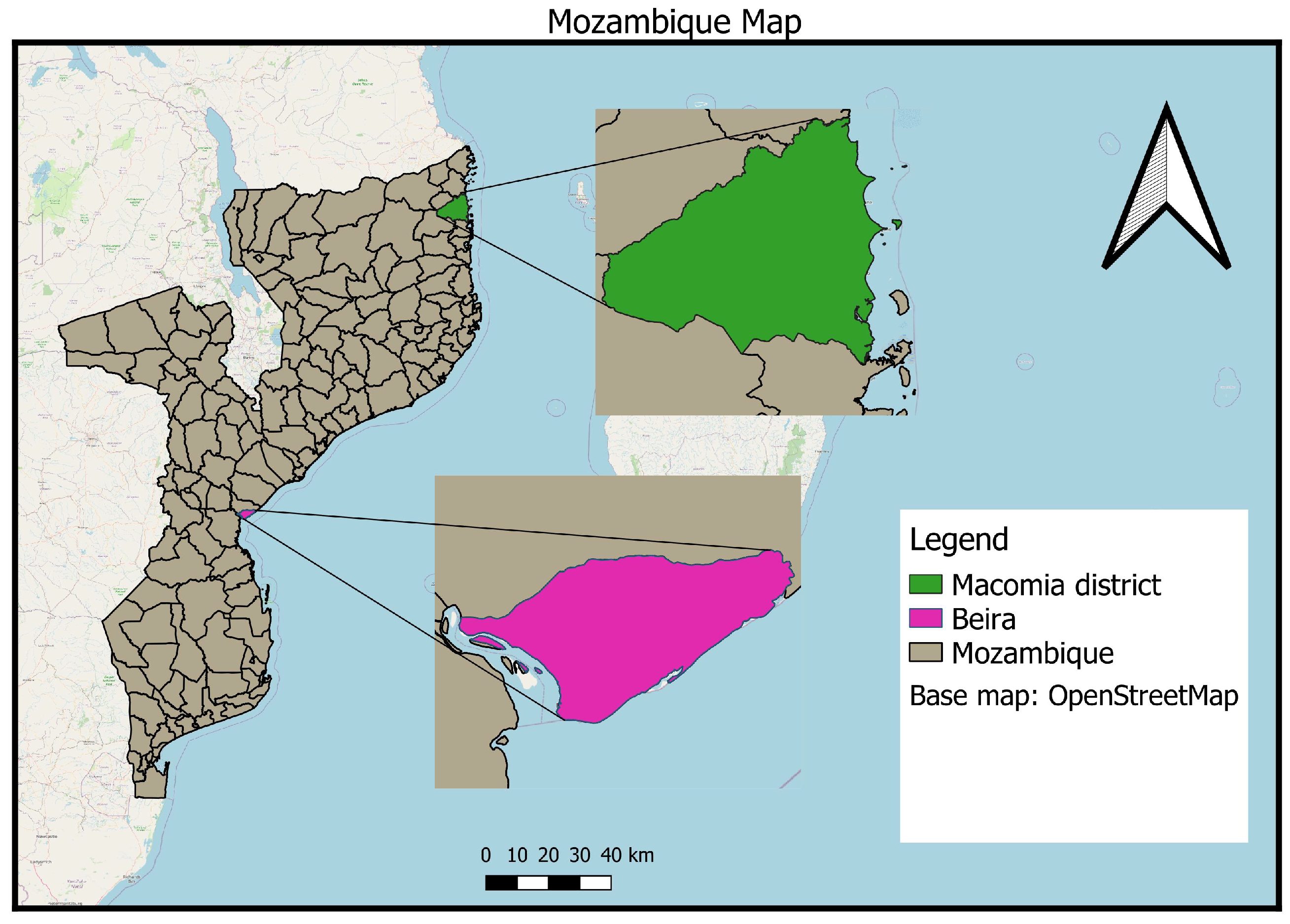
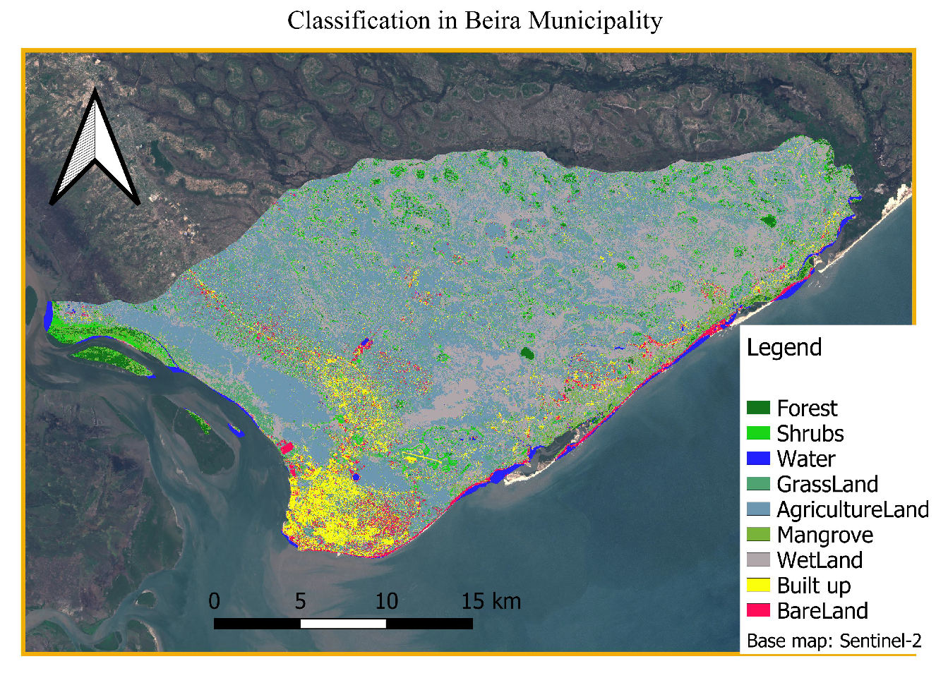
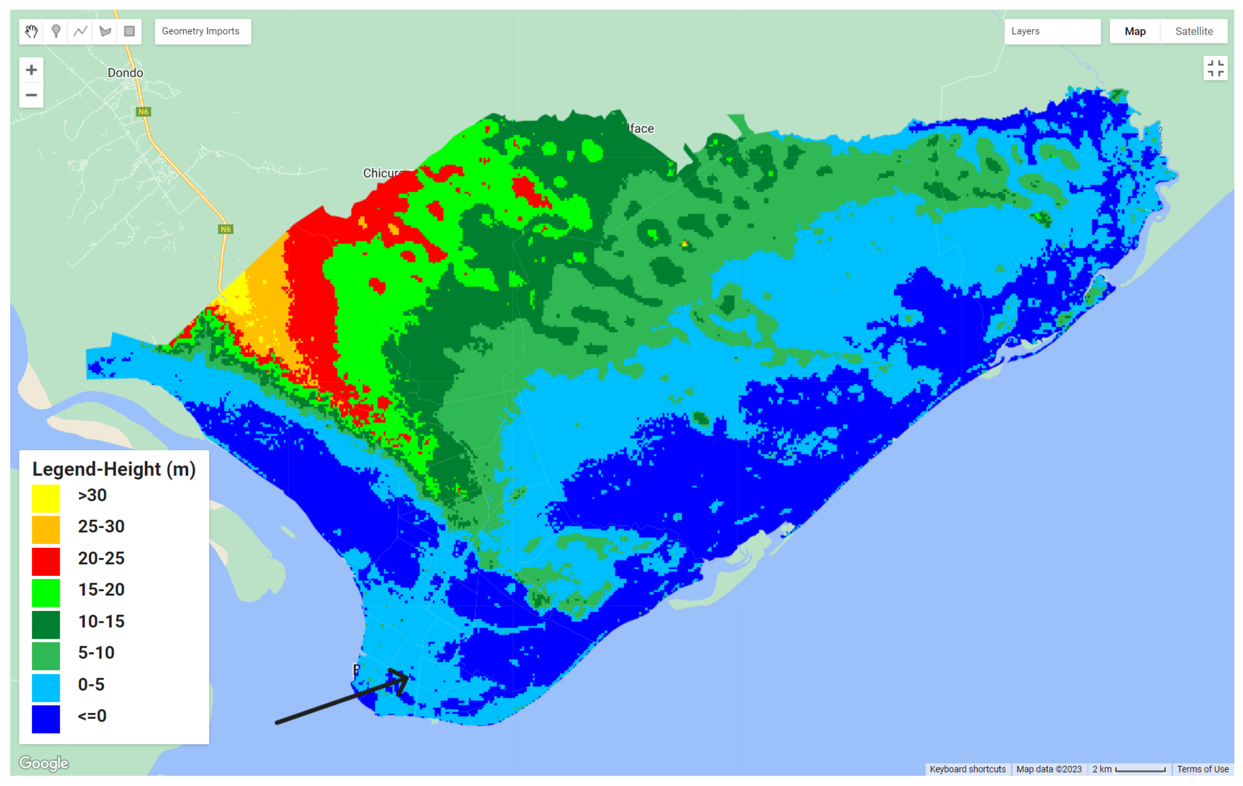
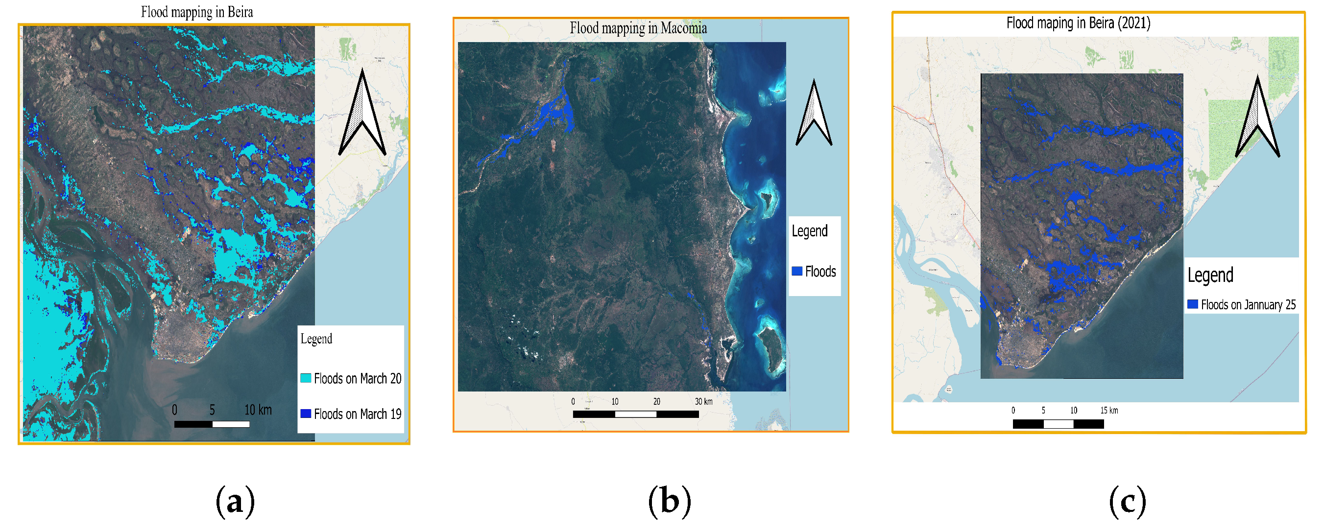
This paper focuses on the Beira municipality (or city of Beira) and Macomia district. Beira is a coastal city, the fourth largest city in Mozambique, located in the central region in Sofala Province (Figure 1). This city has a total area of 633 km${}^2$ and a population of about 500,000 [50]. It is where Pungwe River meets the Indian Ocean, and most areas of this city are under the sea level (Figure 2), making it very prone to flooding. Beira has a very important port that feeds not only the central provinces in Mozambique, but also the inland countries such as Zimbabwe, Malawi and Zambia. 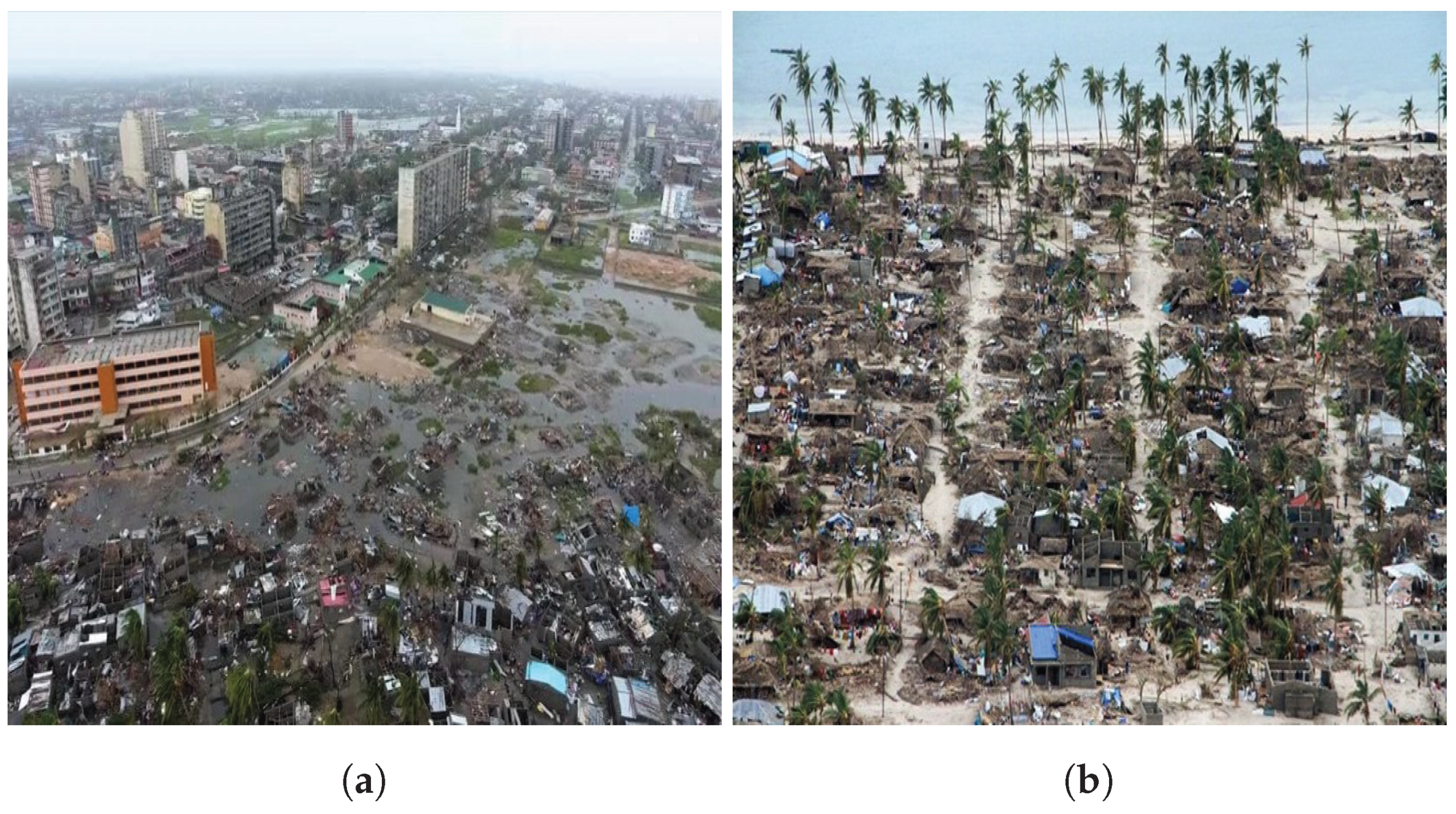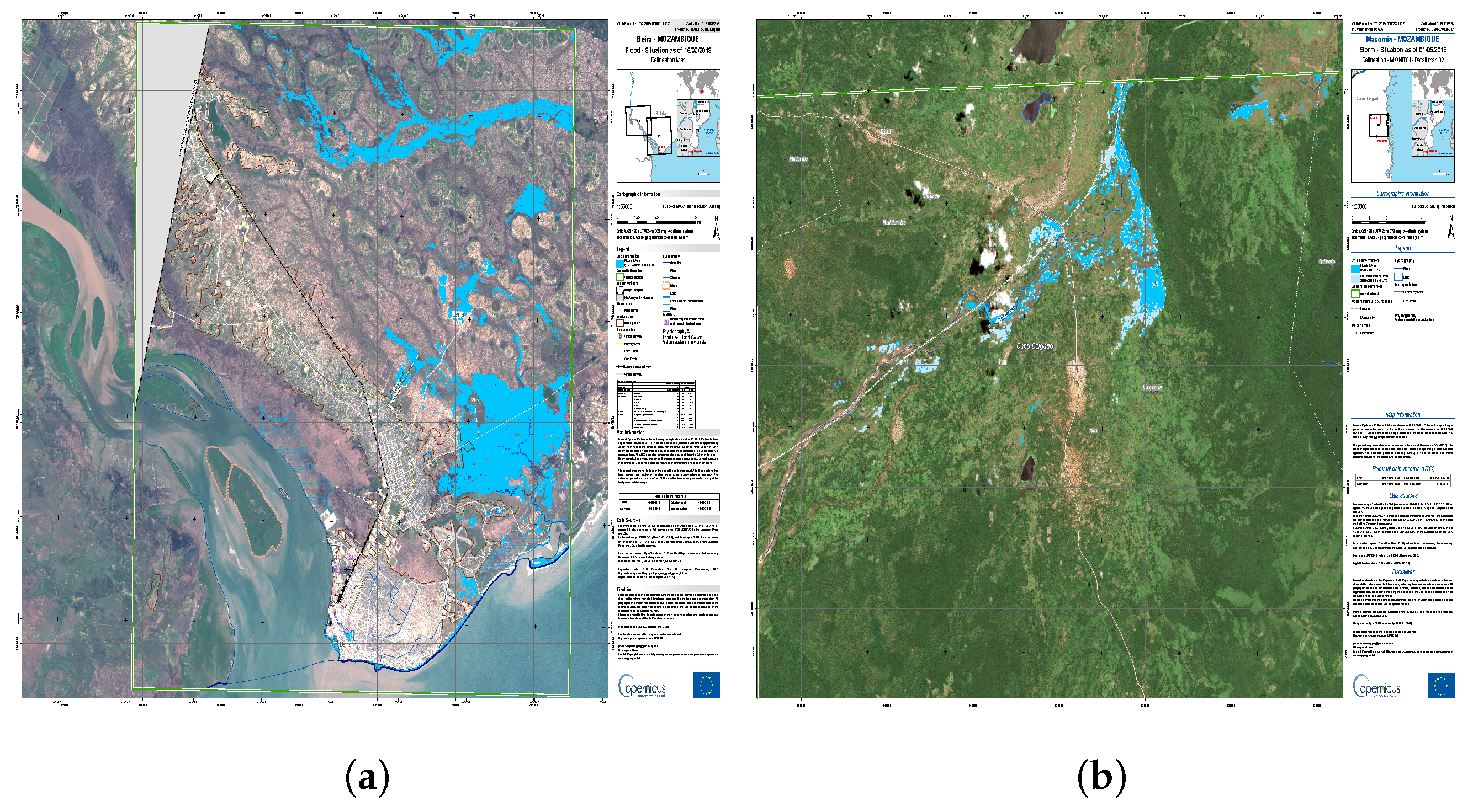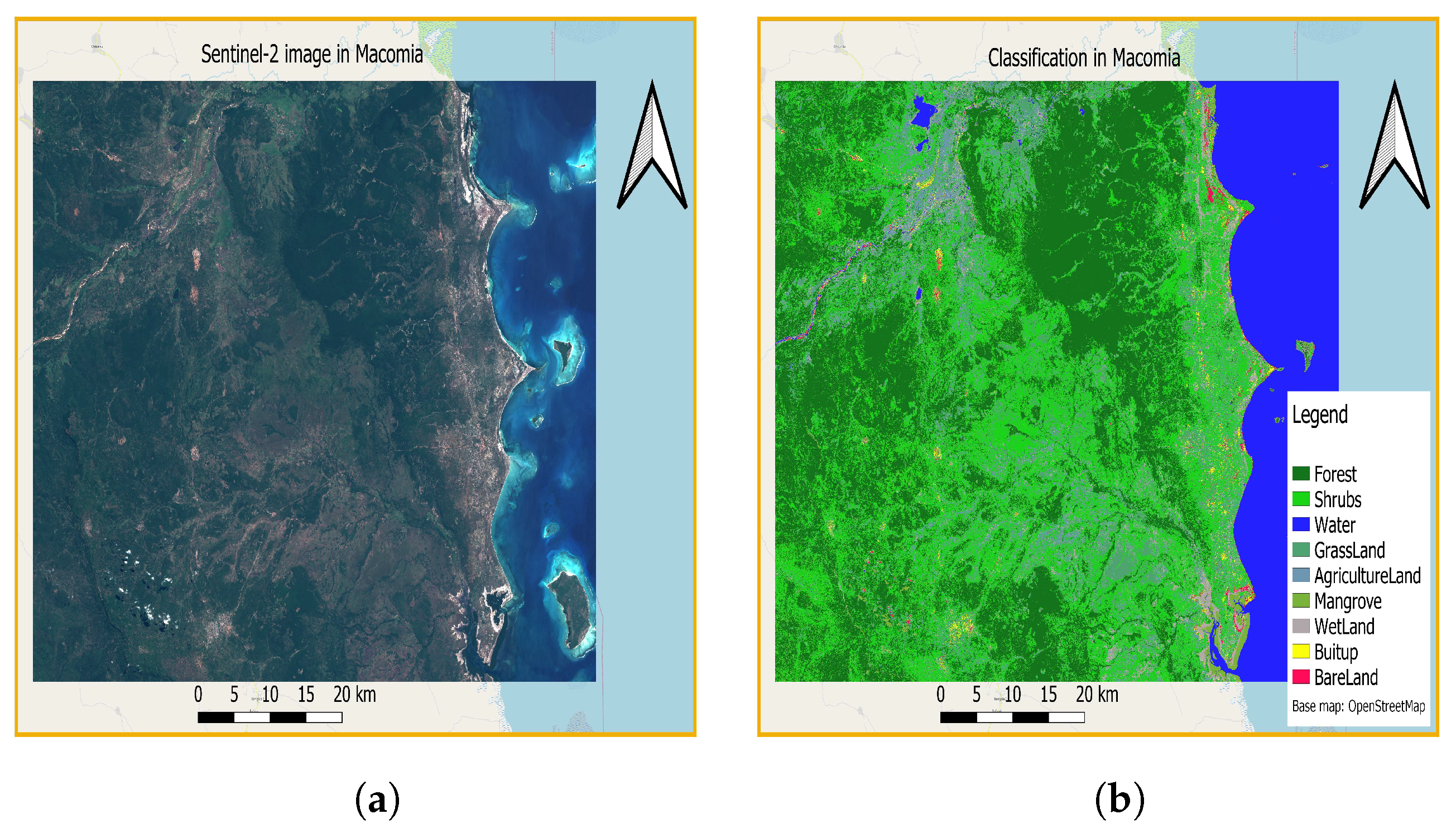Figure 3a displays Beira after TC Idai had hit on 15 March 2019. The second study area, Macomia (Figure 1), is also a coastal district located in the Cabo Delgado province in the northern region of Mozambique. Being bounded by Mocímboa da Praia and Muidumbe districts in the north (also Muidumbe in the northwest), by the Meluco district in the west and southeast, the Quissanga district in the south and by the Indian Ocean in the west, this district has a total area of 4252 km${}^2$ with a total population of about 114,345. With TC Kenneth hitting the Cabo Delgado province on 24 April 2019, this district was the epicenter of the storm (Figure 3b) that came along and because of which 107,836 people were affected (displaced, had houses and crops destroyed), and 33 died [51]. We chose these study areas not only because they were the most affected and important to the country’s economy (mainly for Beira), but also because we have the reference data for accuracy assessment. 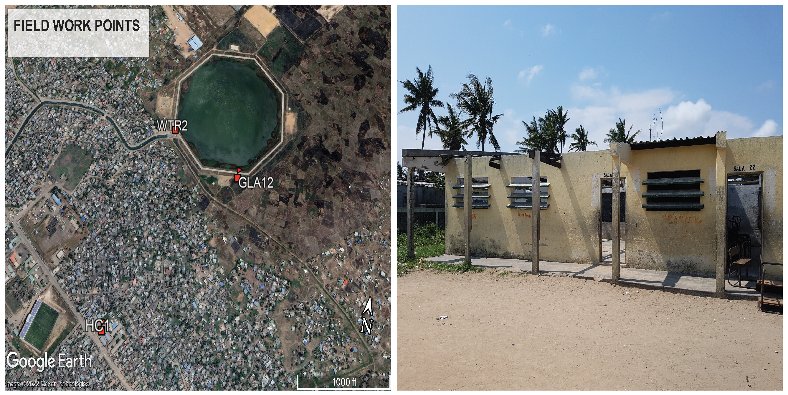Figure 4 displays some GPS (we used a Garmin GPS navigator device) points we collected during the field work in Beira after TC Idai. The points are helpful for LC identification and for visual validation of LC classification results. We collected 15 points for each LC within a neighborhood; therefore, the points are also labeled with numbers from 1 to 15.

We use S1 SAR imagery to map the flooded areas and S2 MSI to assess different LCs that were affected. S1 SAR and S2 MSI are a part of the space component of the Copernicus program of the EU (European Union) and the European Space Agency (ESA) with the aim to manage the environment, study climate change impact, and ensure civil security. During the management of natural disasters, man-made emergency situations and humanitarian crises, the availability of timely and accurate geospatial information over the affected area is of great importance. The specifications of the used data are as follows:

• Sentinel-1 SAR: The S1 mission comprises a constellation of two polar-orbiting satellites (Sentinel-1A and Sentinel-1B) that operate day and night, performing C-band synthetic aperture radar (SAR) imaging, which enables them to acquire imagery regardless of the weather and achieve global coverage every 6 days. It operates at an altitude of 700 km. Sentinel-1A was launched on 3 April 2014, and Sentinel-1B on 25 April 2016. S1 SAR operates with single (VV,VH) or dual (VV+VH, HH+HV) polarizations [52]. S1 SAR has four operating modes, namely: interferometric wide-swath (IW) with 5 m × 20 m spacial resolution and 250 km swath width, stripmap (SM) with 5 m × 5 m spacial resolution and 80 km swath width, extra wide-swath (EW) with 25 m × 40 m spacial resolution and 400 km swath width and wave-mode (WV) with 5 m × 5 m spacial resolution and 20 km by 20 km vignettes every 100 km along the orbit.
  Therefore, in this project, we use S1 imagery for pre- and post-floods (

  Table 3. S1 acquisition dates.

  	Period	Orbit Number	Date	Orbit Pass	Platform
  Beira	Pre-floods	174	13 March 2019	Ascending	Sentinel-1A
  	Post-floods	174	19 March 2019	Ascending	Sentinel-1B
  	Pre-floods	6	2 March 2019	Descending	Sentinel-1A
  	Post-floods	6	20 March 2019	Descending	Sentinel-1B
  	Pre-floods	101	30 July 2020	Ascending	Sentinel-1B
  	Post-floods	174	25 January 2021	Ascending	Sentinel-1A
  Macomia	Pre-floods	57	11 March 2019	Ascending	Sentinel-1B
  	Post-floods	57	28 April 2019	Ascending	Sentinel-1B

  ). The images taken with interferometric wide-swath (IW) acquisition mode and VH polarization.
  Note that the platform Sentinel-1B is no longer operational due to some power supply failure on 23 December 2021. However, Sentinel-1A remains fully operational. More detail about this information can be found in the link available online: https://www.esa.int/Applications/Observing_the_Earth/Copernicus/Sentinel-1/Mission_ends_for_Copernicus_Sentinel-1B_satellite, Assessed: 8 January 2023.
• Sentinel-2 MSI: The S2 mission comprises a constellation of two polar-orbiting optical satellites placed in the same orbit (Sentinel-2A and Sentinel-2B), phased at ${180}^{\circ }$ to each other. Sentinel-2A was launched on 23 June 2015, and Sentinel-2B on 7 March 2017. The multi-spectral instrument (MSI) measures the Earth’s reflected radiance in 13 spectral bands that range from 43 nm to 2190 nm at a spatial resolution of 10–60 m with a swath width of 290. It aims at monitoring the variability inland surface conditions making use of its wide swath and high revisit time. The revisit frequency of each single S2 satellite is 10 days, and the combined constellation revisit is 5 days [53]. In this project, we utilize S2 imagery for LC classification and combine it with the S1 results for damage assessment.

  Table 4. S2 acquisition dates.

  	Image	Orbit Number	Date	Orbit Pass	Platform
  Beira	1	49	2 December 2018	Descending	Sentinel-2B
  Macomia	2	6	7 June 2018	Descending	Sentinel-2A

  shows the S2 data that we used. We use descendant orbit pass images because they were the best (cloud free) images found in the region that cover the whole study area.

Figure 5 shows the reference data produced by Copernicus EMS.

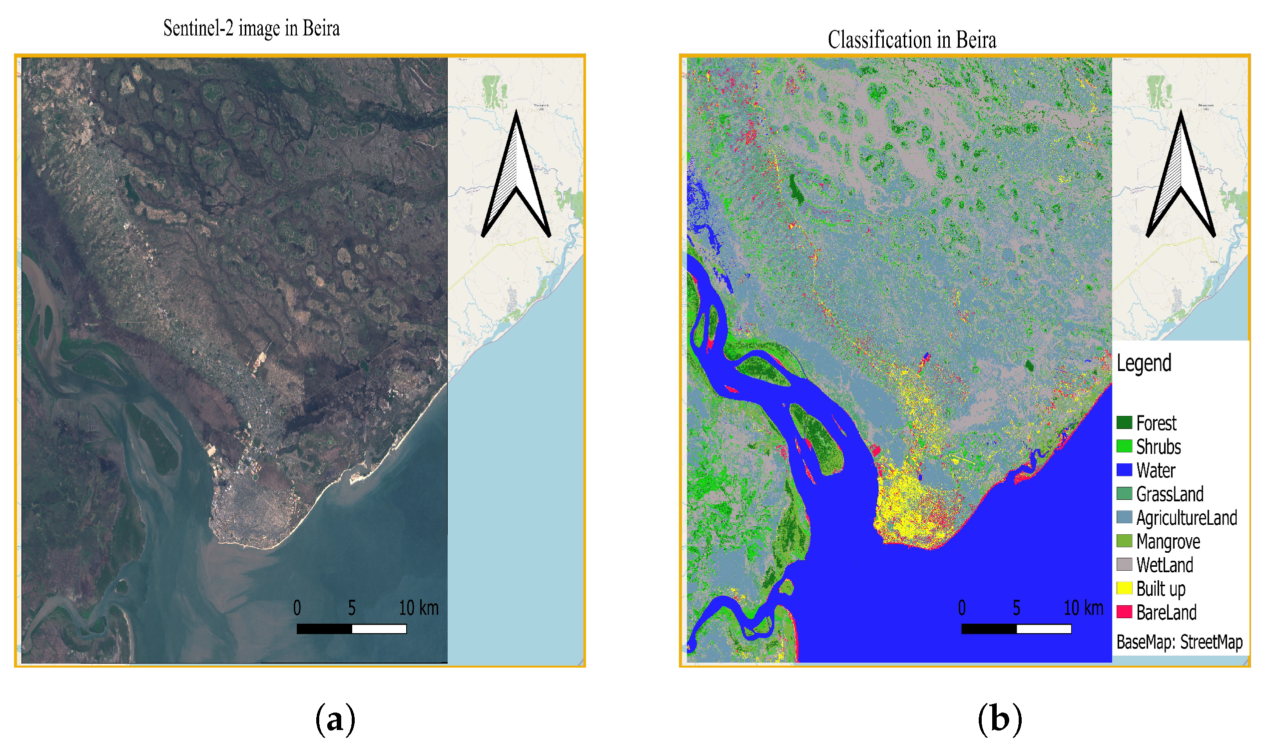
4. Methodology

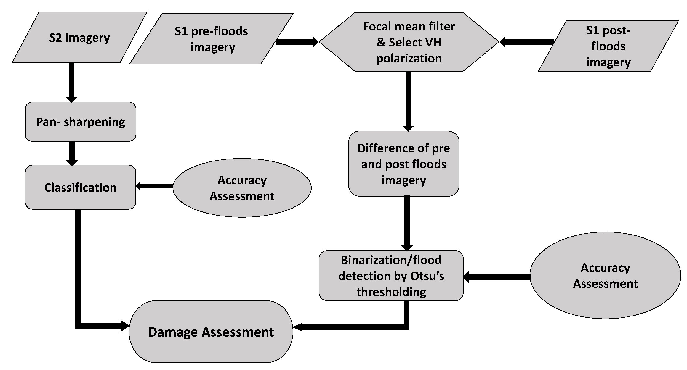
Three main steps to reach the objectives of this work are considered. First, we use S1 data for FM, then we use S2 imagery to classify different LCs (Mangrove, Bare land, Built up Area, Shrubs, Forest, Water, Wetland, Grassland and Agriculture) and finally, we fuse both results to estimate the flooded area for each LC. Given that the data in the Google Earth Engine (GEE) platform are preprocessed, our imagery is geometrically and radiometrically corrected. Additionally, there is no need to download these data given that can they easily be handled within the platform. Thus, the analysis is conducted in GEE and Figure 6 displays the flowchart that summarizes the whole work in this project. The GEE link for the script used to produce the results in this project is https://code.earthengine.google.com/2e933dff4365807cd7ac309deec71c21, Accessed: 19 January 2023. We created the script, except for the Otsu’s thresholding algorithm that is provided in GEE.

4.1. FM Using S1 SAR

For FM (flood detection), we use an image differencing method. This is a traditional pixel-based change detection method. It is well known for its simplicity, easy implementation and understanding [54]. It involves the subtraction of two images (pre- and post-event imagery) pixel-by-pixel and can reach a relatively high accuracy with a low computational cost [21,54], hence its choice for implementation in this project. Additionally, GEE is an online, and shared platform with worldwide coverage, thus, it is highly recommended to use low computational cost techniques to avoid errors (timeout errors or errors due to eventual slow response of the platform). Therefore, to map floods with this method, we first mosaic the pre-flooding S1 images and apply a focal mean filter to remove noise such as lines that appear mainly on the image boundaries or as separation lines on the mosaicked images. The appearance of these lines could be attributed to some sensor problems while imaging. We then apply the same filter on post-flooding images. After that, we compute the difference of the pre- and post-flooding mosaicked images. We choose to use VH polarization imagery due to its high sensitivity to water. Even though VV polarization is often used for FM, VH polarization has also proven to be highly sensitive to water, mainly in rural, swampy or river bank areas [55,56]. Note that Beira city is mostly covered by swampy areas where agriculture is practiced. After calculating the difference, a Gaussian filter is applied to further reduce some speckles. In order to automatically binarize the difference, the Otsu’s thresholding method is used, and then the flooded area is represented by pixels assigned a value of 1, and those with values of 0 are masked out. Additionally, in order to best extract the flooded area, we mask the permanent water along with isolated pixels (pixel groups smaller than 8 pixels) that normally appear after binarization as a result of some mis-detection. We then carry out the accuracy assessment using Copernicus EMS data as a reference (Figure 5). Copernicus EMS services use very high resolution imagery, have a worldwide coverage, and are activated whenever there is a natural disaster. We ingest the Copernicus EMS vectors into GEE and re-project them into the local coordinate system (EPSG:3036) to match Sentinel data. Afterwards, we overlay this vector onto our predicted results, and randomly choose 5000 of the flooded pixels and 5000 of the non-flooded ones over our regions of interest (ROI) to compute the agreement of both results (our prediction and Copernicus EMS results). Some of the statistics we compute use the following formulas that are widely recommend as some of the best practices for accuracy assessment in remote sensing:

$$\mathrm{P}\mathrm{r}\mathrm{e}\mathrm{c}\mathrm{i}\mathrm{s}\mathrm{i}\mathrm{o}\mathrm{n}={\displaystyle \frac{TP}{TP+FP}};$$

(1)

$$\mathrm{R}\mathrm{e}\mathrm{c}\mathrm{a}\mathrm{l}\mathrm{l}={\displaystyle \frac{TP}{TP+FP}};$$

(2)

$$\mathrm{F}1 \mathrm{S}\mathrm{c}\mathrm{o}\mathrm{r}\mathrm{e}={\displaystyle \frac{2\times \mathrm{Recall}\times \mathrm{Precision}}{\mathrm{R}\mathrm{e}\mathrm{c}\mathrm{a}\mathrm{l}\mathrm{l}+\mathrm{P}\mathrm{r}\mathrm{e}\mathrm{c}\mathrm{i}\mathrm{s}\mathrm{i}\mathrm{o}\mathrm{n}}};$$

(3)

$$\mathrm{O}\mathrm{v}\mathrm{e}\mathrm{r}\mathrm{a}\mathrm{l}\mathrm{l} \mathrm{a}\mathrm{c}\mathrm{c}\mathrm{u}\mathrm{r}\mathrm{a}\mathrm{c}\mathrm{y}={\displaystyle \frac{TP+TN}{TP+FP+TN+FN}};$$

(4)

where, $TP$, $FP$, $TN$, and $FN$ stand for true positive, false positive, true negative, and false negative, respectively.

$$\mathrm{k}\mathrm{a}\mathrm{p}\mathrm{p}\mathrm{a}={\displaystyle \frac{P_0-P_e}{1-P_e}}$$

(5)

where $P_0$ is the overall accuracy and $P_e$ is the expected proportion of cases correctly classified by chance. More details about this formula can be found in [57].

Note that we compute the flood detection for a larger area of the Sofala province; however, an accuracy assessment is performed where reference data are available. Certainly, there are some regions within Beira that were not totally covered by the EMS such as Nhangau, and as such we do not include these areas in the accuracy assessment. Nonetheless, considering that Beira tends to have a homogeneous terrain, we assume that our FM results in Beira are representative for the entire Beira municipality and, hence, Nhangau.

4.2. LC Classification Using S2 MSI

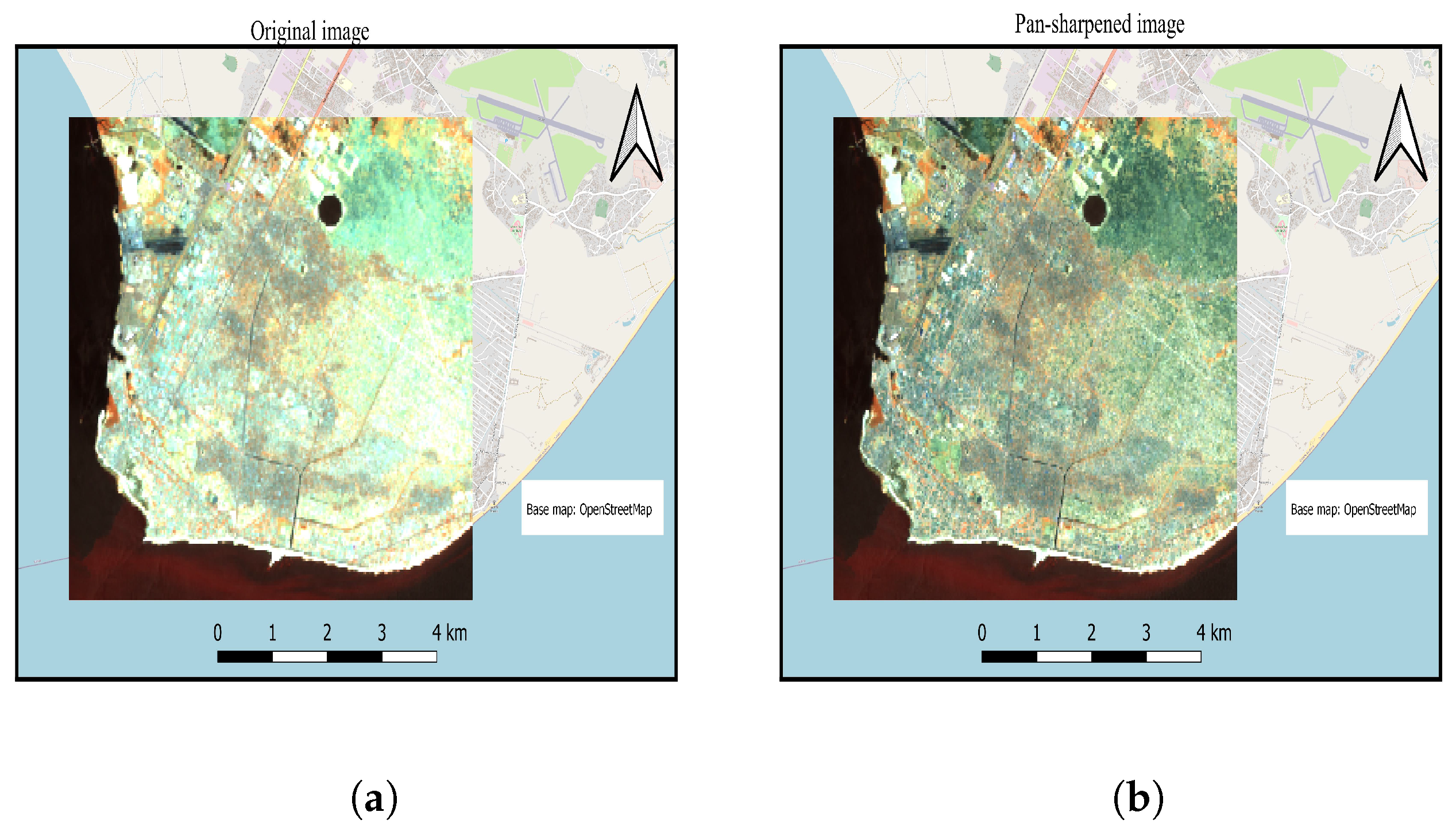
To map the LC, we perform a supervised and pixel-based classification because it allows for exploitation of the authors’ prior information about the study area and helps to select more appropriate training samples to improve the accuracy. We start by the pan-sharpening step to improve the resolution of all the S2 bands with a spatial resolution of 20 m. By applying the Hue-Saturation-Value (HSV) method, we pan-sharpen all these bands utilizing the S2 Band 8 (NIR band) as reference. The S2 band 8 has a 10 m resolution. When the variable Value is replaced by Intensity, the HSV method is called Intensity-Hue-Saturation (IHS) [58,59]. HSV is one of the most used method for pan-sharpening [54] and works as follows:

• We first select bands B5, B6 and B7 and compose an RGB image;
• Transform the RGB imagery into HSV;
• Substitute the value by the panchromatic imagery (S2 band 8);
• Transform back the HSV into the RGB imagery.

Because this method requires three bands at a time, we also apply it to bands 8A, 11, and 12. Thus, the S2 imagery utilized for LC classification consists of 10 bands with a spatial resolution of 10 m. For the second step, we manually collect between 600 and 1500 points (pixels) of data for each class. To collect these points, we draw small polygons comprising around 10 to 30 pixels. Afterwards, we train models with a CART classifier and produce the LC map of the study area. This classifier produces relatively high accuracy results with a low computational cost and complexity [60], and these particularities were import for the choice of this classifier to fulfill the purpose of this project. Finally, the accuracy assessment is performed by computing the confusion matrix, overall accuracy, and kappa coefficient utilizing an independent set of pixels (also containing between 600 and 1500 points for each LC class) as reference data. As with the training points, this set of validation pixels is obtained manually, and due to its high resolution, we explored the base map in GEE during the collection process rather than solely using S2 imagery. The training and validation points are collected from S2 imagery not from the base map; however, the GEE base map imagery is helpful to distinguish different LCs types and minimize errors when collecting training or validation points. That is, with the help of the base map, we can easily locate, on S2 imagery, LCs such as permanent Water, Forest, and Shrubs, but due to the difference of dates between the S2 imagery and the base map, it is highly recommended to pay more attention to LCs such as Built up or Agriculture, as significant differences between the base map and S2 data can be observed. Additionally, we make use of points that were collected on the ground during an in situ fieldwork visit in Beira (Figure 4) to visually compare with our classification. The in situ points also helped identify different LCs during the collection of the training and validation points, and were useful for visual validation of the classification results, but not for the computation of the confusion matrix.

4.3. Damage Assessment

The damage assessment is performed by overlapping both results of FM and classification. We compute the common area between each LC and the flooded area, which results in the flooded area per LC. We also calculate the percentages of flooded areas in both study areas for each LC by dividing the area of each flooded LC by its total area.

5. Results

We first present FM results of both ROIs (Beira municipality and Macomia district) followed by the LC classification results and damage assessment throughout this section.

5.1. FM Results Using S1 SAR

Table 5. Accuracy assessment results for FM in Beira, 19 and 20 March, and Macomia district 28 April both in 2019.

	Beira		Macomia
Statistics	March 19	March 20	April 28
Producer’s Accuracy	0.94	0.93	0.93
User’s Accuracy	0.84	0.82	0.84
Overall Accuracy	0.88	0.87	0.87
Kappa	0.75	0.73	0.74
F1 Score	0.87	0.86	0.85
Precision	0.81	0.80	0.79
Recall	0.93	0.92	0.94

shows the accuracy assessment results of Beira and Macomia. The overall accuracy ranges from 0.87 to 0.88. The kappa coefficient ranges from 0.73 to 0.75, which is substantial, and indicates that there is a considerable agreement between the overall accuracy (what we observed) and expected accuracy. Recall is higher than precision, it ranges from 0.92 to 0.94 against the range of 0.79 to 0.81 for the precision, which indicates the high sensitivity of the method and that it is a bit overoptimistic. However, the F1 score (a metrics that combines both precision and recall) ranges from 0.85 to 0.87, which supports the reliability of the method. Using this metric, we can see that the model performed better in Beira on 19 March. The user’s accuracy reflects the reliability of the classification to the user and is a more relevant measure of the classification’s actual utility in the field. Although the user’s accuracy (ranges from 0.82 to 0.84) is less than the producer’s accuracy in both study areas, it is still very substantial, supporting that the method is trustworthy.

For thresholding, the Otsu’s method was of great help, and we found a mean threshold of $-2.8\pm 0.2$. Notice that the threshold depends greatly on how large the selected ROI is and how many samples of water are included so that the backscattering histogram can be bimodal and easily distinguish water from other LCs. Figure 7a illustrates how the flooding is receding. On 19 March, Beira was severely flooded, but the water is shown to be receding on 20 March. Figure 7c displays the same trend (the same places as in the TC Idai case are flooded) on 25 January 2021, after Beira had been hit again by TC Eloise. Whereas in Beira the water patches are distributed throughout the region, in Macomia (Figure 7b), they are found nearby the rivers, where one river is located in the northern part and the other one goes downward to the Indian Ocean in the southeastern area. A larger flooded area was detected in Beira than in Macomia and that may not be just because of the severity of TC Idai over TC Kenneth, but also the difference in the terrain. Despite this, looking at these results (Figure 7 and Table 5), consistency and extensionality (which means that it can easily be extended to different areas) are qualities that can be perceived from this method.

5.2. LC Classification Using S2 MSI

Figure 8a,b display two images, in which the first is a simple RGB composition of the bands B8A, B11 and B12, and the second is the respective pan-sharpened image. The pen-sharpened image clearly has a higher resolution compared to the original one. Although the results are not presented here, we repeat the pen-sharpening process for bands B5, B6 and B7. Figure 9a and Figure 10a show RGB images composed by the pan-sharpened bands including bands B2, B3, B4, and B8, and thus, they comprise 10 bands. Figure 9b and Figure 10b display the LC classification results (Figure 11 is a part of Figure 9b, it displays classification results only for the city of Beira with its 26 neighborhoods), and

Table 6. Accuracy assessment results for classification in Beira and Macomia, 2019.

	Producer’s Acc.		User’s Acc.
Classes	Macomia	Beira	Macomia	Beira
Built up	0.68	0.83	0.91	0.91
Bareland	0.93	0.72	0.80	0.82
Forest	0.99	0.95	0.99	0.89
Shrubs	0.88	0.67	0.81	0.90
Grassland	0.93	0.69	0.92	0.75
Water	1.00	1.00	0.98	1.00
Wetland	0.82	0.92	0.88	0.85
Mangrove	0.99	0.76	0.99	0.88
Agriculture	0.82	0.95	0.86	0.86
	Macomia		Beira
Overall accuracy	95%		90%
Kappa	0.94		0.80

shows the respective accuracy assessment results where the overall accuracy is of 90–95% and a kappa of 0.80–0.94. The kappa coefficient shows that there is a substantial agreement between predicted and expected results in this classification. The producer’s accuracy (or errors of omission because the producer’s accuracy is the complement of an omission error) column shows false negatives and reflects the points that are included in the category while they really do not belong to that category. The Shrubs class in Beira has the lowest producer’s accuracy (0.67), equivalent to an omission error of (0.33), and it indicates that there is a number of pixels belonging to this class that were classified as other classes. This situation is also observed with Grassland in Beira (producer’s accuracy of 0.69) and the Build up class in Macomia (producer’s accuracy 0.68). On the other hand, the user’s accuracy (or commission error), which tells how often the class on the map will actually be present on the ground, is considerably high for both regions. That is, within the predicted pixels in each class there are a few that were misclassified.

5.3. Damage Assessment

Wetland is predominant and is the most flooded in Beira with 19.73% of the flooded area out of 538.54 km${}^2$ of its total area, followed by Agriculture, which has a total area of about 419 km${}^2$ and 13.08% of the flooded area on 19 March (

Table 7. Flooded areas in km${}^2$ on 19 and 20 March 2019 and the percentages of flooded areas for each LC in Beira. TA and Diff stand for total area and difference flooded areas on 19 and 20 March, respectively.

Classes	TA (km${}^2$)	Flooded Area (km${}^2$)		Flooded Area (%)		Diff (km${}^2$)
		19 March	20 March	19 March	20 March
Built up	43.75	1.29	1.11	3.00	2.53	0.18
Bareland	27.36	2.39	1.28	8.74	4.67	1.11
Forest	61.03	2.87	2.14	4.41	3.51	0.73
Shrubs	89.91	10.21	6.65	11.35	7.62	3.56
Mangrove	32.46	0.71	0.59	2.55	1.81	0.12
Agriculture	419.69	54.90	29.18	13.08	7.16	25.72
Grassland	114.46	8.32	4.54	7.27	3.85	3.78
Wetland	538.54	106.24	69.10	19.73	12.83	37.14

). This is not surprising because Beira is generally swampy under the sea level. Sometimes, some Bareland areas in Beira are Wetland, which depends on the season, i.e., some Bareland areas are usually Wetland, they just dry up and become Bareland due to long periods without rains. Furthermore, groundwater is too close to the surface, and when the rain comes easily, the city inundates because the surface fails to absorb it in time. On the other hand, those features make Beira a good place to grow cultures such as rice, sweet potatoes, lettuce and other vegetables. Notice that in both ROIs we have Agriculture with flooded areas being significantly high, a fact that raised concerns about the guarantees of food for the locals. It is also important to highlight that the majority of Mozambicans are dependent on subsistence agriculture, and these results once again support that fact. Huge agricultural lands are often found in many districts of Mozambique just like Beira and Macomia (see that Macomia has about 613 km${}^2$ of agriculture,

Table 8. Flooded areas in km${}^2$ and the percentages for each LC that was classified in Macomia and Beira. The results from 28 April 2019, in Macomia and 25 January 2021, in Beira.

Classes	Total  Area (km${}^2$ )		Flooded Area (km${}^2$ )		(%)  of  Flooded  Area
	Macomia	Beira${}^{\left(2021\right)}$	Macomia	Beira${}^{\left(2021\right)}$	Macomia	B${}^{\left(2021\right)}$
Built up	6.56	43.75	0.81	0.95	12.30	2.20
Bareland	3.26	27.39	0.19	1.06	5.85	3.86
Forest	145.87	61.03	2.23	1.27	1.52	2.25
Shrubs	234.74	89.91	6.64	1.70	2.83	1.89
Mangrove	10.45	32.46	0.28	0.34	2.68	1.06
Agriculture	613.98	419.69	10.27	19.07	1.67	4.54
Grassland	83.56	114.46	9.25	2.19	11.08	1.91
Wetland	43.89	538.54	8.35	61.16	19.00	11.34

). The difference column (Diff) in Table 7 helps understand how the flooding receded from 19 March to 20 within each LC. In Wetland, the water receded faster followed by Agriculture, which is a good sign; however, it may happen that the water dragged the crops away with it, destroying all those fields. Mangrove has the lowest difference and appears as the least affected class, which suggest that there was no considerable destruction and the water continued following its normal paths. With less causalities reported than in the case of TC Idai, TC Eloise hit Beira in January, 2021, and the damages were close to those of TC Idai (Table 8). Agriculture continues to be the second most affected, and Mangrove the least affected.

6. Discussion

6.1. FM Results

In Beira, we were able to retrieve image data for two days (19 and 20 March 2019) and analyze how fast the water was receding, whereas in Macomia, the available data were only for a single day. However, it was possible to have a general and interesting overview of the flooding in both ROIs. The terrain difference between Beira and Macomia had less of an effect than we expected. Our approach was able to capture the flooded area significantly well in both study areas with considerably high accuracy that is not far from what was obtained with more sophisticated approaches such as in [16,17,38]. The narrow ranges in all the statistics highlight the consistency of the approach. Thus, once again, the method was shown to have a high extensionality with a low computational cost as presented in [40]. The FM results presented in this paper fortify the evidence supporting that this flood detection method is consistent, tractable and simple to apply in rapid FM requirements.

Despite the fact that we validated our results only within the regions covered by Copernicus EMS, for damage assessment in Beira, we included Nhangau. With the inclusion of Nhangau, we did not just cover the entire Beira municipality, but also capitalized an important and strategic region to understand the severity of the damages. This is because, although Nhangau is not densely inhabited, it has considerable agricultural lands that serve as sources of food for the local population. Therefore, even though we perform no formal validation in Nhangau, we assume that the quality of the flooding is as representative as in our validated region. Moreover, there are no reference results from the EMS for the TC Eloise flooding; however, mapping floods from this TC is important to give an insight that endorses how the consequences of climate changes are affecting Mozambique [61].

6.2. LC Classification and Damage Assessment

The results achieved in this project about LC classification were satisfactory, and the accuracy is comparable to that obtained in [48] (they had an overall accuracy of 97.71% and kappa of 0.9477 for supervised classification). They are also in agreement with what we have seen during the field work conducted right after the TCs, and with the ground points that we collected.

The damage assessment results highlighted that Beira is dominated by wetlands and vast agricultural areas, as its inhabitants are strongly dependent on it. Thus, the devastation of agricultural areas has a direct impact on the local inhabitants and poses high food insecurity. The suburban constructions are on wetland, grassland or agricultural areas, which implies that inundations of theses areas may cause human displacement. The challenging fact about these constructions is that they are too small and have considerably different roof types from city buildings (some use grass), which means their reflectance can easily be mistaken for other LC classes, hence the low accuracy on the Built up class. On the other hand, Beira and Macomia are coastal areas, but differently from Macomia, Beira has been facing erosion and deforestation for long time, and the causes are attributed to human activities or the impacts of climate change [61,62,63]. The destruction of mangroves and forests, as shown in Table 7 and Table 8, increases the risk of erosion, which raises concerns about the long term existence of the city. Moreover, it can be seen that areas flooded during TC Eloise are almost the same as in the case of TC Idai, which highlights a flooding pattern in Beira. This fact can help the local structures with better planning of their land use, especially in urban planning. Therefore, although the approach that was implemented is not new, one of the most remarkable results presented in this project is the analysis of how the floods receded in Beira during two consecutive days and the comparison of the results in different years. This information can also help identify risky and non-risky areas so that the locals know where to shelter themselves whenever there is a new flood event. Human displacement due to flooding is recurrent not only in Beira, but throughout the country, and the local structures are repeatedly impelled to find better places for resettlement.

Although S1 imagery comes with a relatively high spatial resolution, the FM experiments show that some flooded pixels are not well-classified. Some of these misclassified pixels belong to some small natural depressions (basins). These depressions on the Earth’s surface occur everywhere and are able to retain water in a flood event. Inside a particular depression, if one pixel at certain elevation is correctly classified as flooded, then it should be expected that the other pixels at the same elevation are likely flooded. Some of these bottlenecks could be mitigated by exploiting information from Digital Elevation Models (DEM), as we can estimate the depth of the water in flooded areas and correct some misclassified pixels. We also need to note some limitations of our FM validation, as the Copernicus EMS results were not available for all the affected districts, including the case of TC Eloise, where no EMS results were available at all. Furthermore, although the S1 and S2 data are freely available in GEE, some delays in their availability after a disaster event may occur. Nevertheless, we find the combination of S1 and S2 very useful for FM and damage assessment. By harnessing the arsenal of GEE functions, we were able to handle all data online and make sure that the FM can be obtained in near real-time. Moreover, GEE allows for the quick ingestion of other ancillary sources.

7. Conclusions and Future Research

In this work, we presented an automatic near real-time algorithm for FM by exploring the potential of S1 data in GEE. We also explored the capabilities of S2 and its synergy with S1 for damage assessment. The algorithm for FM showed an overall accuracy of 87–88% and kappa of 0.73–0.75 when compared directly with Copernicus EMS results, and this shows substantial agreement with the reference data. However, it produced higher recall than precision, indicating that it was a bit overoptimistic. Low ranges in all statistics mainly for the F1 Score (ranges from 0.85 to 0.87) highlighted the reliability and consistency of this method. Moreover, the method showed that it can be securely replicated and still yield results with high accuracy, which is a great advantage for the purpose of this project, which is to provide the local structures (in Mozambique) with reliable tools for better planning. We extracted, among others, damaged built up and agricultural areas, as they carry vital information to enhance local planning efforts. The fusion of S1-based FM results with a S2-based LC classification showed remarkable potential for rapid damage assessment. The classification overall accuracy was 90–95% with a kappa of 0.80–94, which also shows high alignment of the results with the reference data. The user’s accuracy, which reflects the reliability of the classification to the user, is very high (ranges from 0.75 to 1.0) for both study areas, and together with other statistics indicates that the method performed relatively well, and that the classification results are trustworthy. Given that Beira is largely swampy, it was challenging to distinguish Mangrove from Shrubs and Grassland; however, it was possible to create an adequate separation of those classes. Agreeing with our expectations, Wetland was the most affected area in Beira (we found flooded area of 106.24 km${}^2$ ), while agricultural land was considerably impacted by flooding in both ROIs. This is due to the composition of Beira LC, which is under the sea level, while the livelihoods of its inhabitants in both regions make them very dependent on subsistence agriculture.

Furthermore, the FM experiments showed that some of the misclassified pixels belong to some small natural depressions. These depressions on the Earth’s surface occur everywhere and are able to retain water in a flood event. Inside a particular depression, if one pixel at a certain elevation is correctly classified as flooded, then it should be expected that the other pixels at the same elevation are likely flooded. Some of these bottlenecks could be mitigated by exploiting information from DEM, as we can estimate the depth of the water in flooded areas and correct the misclassified pixels. Therefore, for improving the flood detection in the risk zones, further investigation of DEM information should be considered.

References

1. Karlsson, J.M.; Arnberg, W. Quality analysis of SRTM and HYDRO1K: A case study of flood inundation in Mozambique. Int. J. Remote Sens. 2011, 32, 267–285. [Google Scholar] [CrossRef]
2. Asante, K.O.; Macuacua, R.D.; Artan, G.A.; Lietzow, R.W.; Verdin, J.P. Developing a flood monitoring system from remotely sensed data for the Limpopo basin. IEEE Trans. Geosci. Remote Sens. 2007, 45, 1709–1714. [Google Scholar] [CrossRef]
3. Kondo, H.; Seo, N.; Yasuda, T.; Hasizume, M.; Koido, Y.; Ninomiya, N.; Yamamoto, Y. Post-flood—infectious diseases in Mozambique. Prehospital Disaster Med. 2002, 17, 126–133. [Google Scholar] [CrossRef] [PubMed]
4. McElwee, R. Tropical Storm Dineo Hits Mozambique. Aljazeera. 6 November 2018. Available online: https://www.aljazeera.com/news/2017/02/tropical-storm-dineo-hits-mozambique-170216105245838.html (accessed on 2 February 2019).
5. Whatchers, T. Floods in Mozambique. 2018. Available online: https://watchers.news/2018/01/25/floods-in-mozambique-leave-11-dead-up-to-15-000-homes-destroyed/ (accessed on 19 February 2019).
6. Asante, K.; Brito, R.; Brundrit, G.; Epstein, P.; Nussbaumer, P.; Patt, A. Study on the Impact of Climate Change on Disaster Risk in Mozambique: Synthesis Report. Maputo: National Institute for Disaster Management. May 2009. Available online: https://www.biofund.org.mz/biblioteca_virtual/synthesis-report-ingc-climate-change-report-study-on-the-impact-of-climate-change-on-disaster-risk-in-mozambique/ (accessed on 29 January 2023).
7. Frey, A. Mozambique’s INGC to Step Up Use of Drones for Natural Disaster Risk Management. Club of Mozambique. 15 November 2017. Available online: https://clubofmozambique.com/news/mozambiques-ingc-to-step-up-use-of-drones-for-natural-disaster-risk-management/ (accessed on 23 February 2019).
8. Ban, Y.; Yousif, O.; Hu, H. Fusion of SAR and optical data for urban land cover mapping and change detection. Glob. Urban Monit. Assess. Earth Obs. 2014, 353. [Google Scholar]
9. Ban, Y.; Webber, L.; Gamba, P.; Paganini, M. EO4Urban: Sentinel-1A SAR and Sentinel-2A MSI data for global urban services. In Proceedings of the 2017 Joint Urban Remote Sensing Event (JURSE), Dubai, United Arab Emirates, 6–8 March 2017; IEEE: Piscataway, NJ, USA, 2017; pp. 1–4. [Google Scholar]
10. Singh, A. Review article digital change detection techniques using remotely-sensed data. Int. J. Remote Sens. 1989, 10, 989–1003. [Google Scholar] [CrossRef]
11. Tewkesbury, A.P.; Comber, A.J.; Tate, N.J.; Lamb, A.; Fisher, P.F. A critical synthesis of remotely sensed optical image change detection techniques. Remote Sens. Environ. 2015, 160, 1–14. [Google Scholar] [CrossRef]
12. Haas, J.; Ban, Y. Urban growth and environmental impacts in Jing-Jin-Ji, the Yangtze, River Delta and the Pearl River Delta. Int. J. Appl. Earth Obs. Geoinf. 2014, 30, 42–55. [Google Scholar] [CrossRef]
13. Ban, Y.; Yousif, O.A. Multitemporal spaceborne SAR data for urban change detection in China. IEEE J. Sel. Top. Appl. Earth Obs. Remote Sens. 2012, 5, 1087–1094. [Google Scholar] [CrossRef]
14. Buchanan, G.M.; Butchart, S.H.; Dutson, G.; Pilgrim, J.D.; Steininger, M.K.; Bishop, K.D.; Mayaux, P. Using remote sensing to inform conservation status assessment: Estimates of recent deforestation rates on New Britain and the impacts upon endemic birds. Biol. Conserv. 2008, 141, 56–66. [Google Scholar] [CrossRef]
15. Chowdhury, R.R. Driving forces of tropical deforestation: The role of remote sensing and spatial models. Singap. J. Trop. Geogr. 2006, 27, 82–101. [Google Scholar] [CrossRef]
16. DeVries, B.; Huang, C.; Armston, J.; Huang, W.; Jones, J.W.; Lang, M.W. Rapid and robust monitoring of flood events using Sentinel-1 and Landsat data on the Google Earth Engine. Remote Sens. Environ. 2020, 240, 111664. [Google Scholar] [CrossRef]
17. Twele, A.; Cao, W.; Plank, S.; Martinis, S. Sentinel-1-based flood mapping: A fully automated processing chain. Int. J. Remote Sens. 2016, 37, 2990–3004. [Google Scholar] [CrossRef]
18. Tralli, D.M.; Blom, R.G.; Zlotnicki, V.; Donnellan, A.; Evans, D.L. Satellite remote sensing of earthquake, volcano, flood, landslide and coastal inundation hazards. ISPRS J. Photogramm. Remote Sens. 2005, 59, 185–198. [Google Scholar] [CrossRef]
19. Jain, S.K.; Singh, R.; Jain, M.; Lohani, A. Delineation of flood-prone areas using remote sensing techniques. Water Resour. Manag. 2005, 19, 333–347. [Google Scholar] [CrossRef]
20. Brivio, P.; Colombo, R.; Maggi, M.; Tomasoni, R. Integration of remote sensing data and GIS for accurate mapping of flooded areas. Int. J. Remote Sens. 2002, 23, 429–441. [Google Scholar] [CrossRef]
21. Bindschadler, R.A.; Scambos, T.A.; Choi, H.; Haran, T.M. Ice sheet change detection by satellite image differencing. Remote Sens. Environ. 2010, 114, 1353–1362. [Google Scholar] [CrossRef]
22. Sohl, T.L. Change analysis in the United Arab Emirates: An investigation of techniques. Photogramm. Eng. Remote Sens. 1999, 65, 475–484. [Google Scholar]
23. Dalecki, M.; Willits, F.K. Examining change using regression analysis: Three approaches compared. Sociol. Spectr. 1991, 11, 127–145. [Google Scholar] [CrossRef]
24. Bates, B.C.; Chandler, R.E.; Bowman, A.W. Trend estimation and change point detection in individual climatic series using flexible regression methods. J. Geophys. Res. Atmos. 2012, 117, D16. [Google Scholar] [CrossRef]
25. Celik, T. Unsupervised change detection in satellite images using principal component analysis and k-means clustering. IEEE Geosci. Remote Sens. Lett. 2009, 6, 772–776. [Google Scholar] [CrossRef]
26. Bovolo, F.; Bruzzone, L. A theoretical framework for unsupervised change detection based on change vector analysis in the polar domain. IEEE Trans. Geosci. Remote Sens. 2006, 45, 218–236. [Google Scholar] [CrossRef]
27. Alphan, H.; Doygun, H.; Unlukaplan, Y.I. Post-classification comparison of land cover using multitemporal Landsat and ASTER imagery: The case of Kahramanmaraş, Turkey. Environ. Monit. Assess. 2009, 151, 327–336. [Google Scholar] [CrossRef] [PubMed]
28. Dai, X.; Khorram, S. Remotely sensed change detection based on artificial neural networks. Photogramm. Eng. Remote Sens. 1999, 65, 1187–1194. [Google Scholar]
29. Gamba, P.; Dell’Acqua, F.; Lisini, G. Change detection of multitemporal SAR data in urban areas combining feature-based and pixel-based techniques. IEEE Trans. Geosci. Remote Sens. 2006, 44, 2820–2827. [Google Scholar] [CrossRef]
30. Xiao, P.; Zhang, X.; Wang, D.; Yuan, M.; Feng, X.; Kelly, M. Change detection of built-up land: A framework of combining pixel-based detection and object-based recognition. ISPRS J. Photogramm. Remote Sens. 2016, 119, 402–414. [Google Scholar] [CrossRef]
31. Yousif, O.; Ban, Y. A novel approach for object-based change image generation using multitemporal high-resolution SAR images. Int. J. Remote Sens. 2017, 38, 1765–1787. [Google Scholar] [CrossRef]
32. Giustarini, L.; Hostache, R.; Matgen, P.; Schumann, G.J.P.; Bates, P.D.; Mason, D.C. A change detection approach to flood mapping in urban areas using TerraSAR-X. IEEE Trans. Geosci. Remote Sens. 2012, 51, 2417–2430. [Google Scholar] [CrossRef]
33. Jianya, G.; Haigang, S.; Guorui, M.; Qiming, Z. A review of multi-temporal remote sensing data change detection algorithms. Int. Arch. Photogramm. Remote Sens. Spat. Inf. Sci. 2008, 37, 757–762. [Google Scholar]
34. Ban, Y.; Yousif, O. Change Detection Techniques: A Review. In Multitemporal Remote Sensing: Methods and Applications; Ban, Y., Ed.; Springer International Publishing: Cham, Switzerland, 2016; pp. 19–43. [Google Scholar] [CrossRef]
35. López-Serrano, P.M.; Corral-Rivas, J.J.; Díaz-Varela, R.A.; Álvarez-González, J.G.; López-Sánchez, C.A. Evaluation of radiometric and atmospheric correction algorithms for aboveground forest biomass estimation using Landsat 5 TM data. Remote Sens. 2016, 8, 369. [Google Scholar] [CrossRef]
36. Paolini, L.; Grings, F.; Sobrino, J.A.; Jiménez Muñoz, J.C.; Karszenbaum, H. Radiometric correction effects in Landsat multi-date/multi-sensor change detection studies. Int. J. Remote Sens. 2006, 27, 685–704. [Google Scholar] [CrossRef]
37. Martinis, S.; Twele, A.; Voigt, S. Towards operational near real-time flood detection using a split-based automatic thresholding procedure on high resolution TerraSAR-X data. Nat. Hazards Earth Syst. Sci. 2009, 9, 303–314. [Google Scholar] [CrossRef]
38. Li, Y.; Martinis, S.; Wieland, M.; Schlaffer, S.; Natsuaki, R. Urban Flood Mapping Using SAR Intensity and Interferometric Coherence via Bayesian Network Fusion. Remote Sens. 2019, 11, 2231. [Google Scholar] [CrossRef]
39. Schumann, G.J.P.; Moller, D.K. Microwave remote sensing of flood inundation. Phys. Chem. Earth Parts A/B/C 2015, 83, 84–95. [Google Scholar] [CrossRef]
40. Clement, M.; Kilsby, C.; Moore, P. Multi-temporal synthetic aperture radar flood mapping using change detection. J. Flood Risk Manag. 2018, 11, 152–168. [Google Scholar] [CrossRef]
41. Uddin, K.; Matin, M.A.; Meyer, F.J. Operational flood mapping using multi-temporal sentinel-1 SAR images: A case study from Bangladesh. Remote Sens. 2019, 11, 1581. [Google Scholar] [CrossRef]
42. Canty, M.J.; Nielsen, A.A.; Conradsen, K.; Skriver, H. Statistical Analysis of Changes in Sentinel-1 Time Series on the Google Earth Engine. Remote Sens. 2020, 12, 46. [Google Scholar] [CrossRef]
43. Arora, S.; Acharya, J.; Verma, A.; Panigrahi, P.K. Multilevel thresholding for image segmentation through a fast statistical recursive algorithm. Pattern Recognit. Lett. 2008, 29, 119–125. [Google Scholar] [CrossRef]
44. Long, S.; Fatoyinbo, T.E.; Policelli, F. Flood extent mapping for Namibia using change detection and thresholding with SAR. Environ. Res. Lett. 2014, 9, 035002. [Google Scholar] [CrossRef]
45. Kittler, J.; Illingworth, J. Minimum error thresholding. Pattern Recognit. 1986, 19, 41–47. [Google Scholar] [CrossRef]
46. Nandi, I.; Srivastava, P.K.; Shah, K. Floodplain mapping through support vector machine and optical/infrared images from Landsat 8 OLI/TIRS sensors: Case study from Varanasi. Water Resour. Manag. 2017, 31, 1157–1171. [Google Scholar] [CrossRef]
47. Amarnath, G. An algorithm for rapid flood inundation mapping from optical data using a reflectance differencing technique. J. Flood Risk Manag. 2014, 7, 239–250. [Google Scholar] [CrossRef]
48. Kordelas, G.A.; Manakos, I.; Aragonés, D.; Díaz-Delgado, R.; Bustamante, J. Fast and automatic data-driven thresholding for inundation mapping with Sentinel-2 data. Remote Sens. 2018, 10, 910. [Google Scholar] [CrossRef]
49. Dao, P.D.; Liou, Y.A. Object-based flood mapping and affected rice field estimation with Landsat 8 OLI and MODIS data. Remote Sens. 2015, 7, 5077–5097. [Google Scholar] [CrossRef]
50. Spekker, H.; Kleinefeld, B. Climate Change Adaption Strategies in Developing Countries–Exemplary Flood and Erosion Protection Projects in Mozambique. Coast. Struct. 2019, 2019, 1066–1074. [Google Scholar]
51. INGC; OCHA. Mozambique Cyclone Kenneth: Assessment Report—Macomia Town, Macomia District, Cabo Delgado 12 May 2019; INGC and OCHA: Pemba, Mozambique, 2019; Available online: https://reliefweb.int/report/mozambique/mozambique-cyclone-kenneth-assessment-report-macomia-town-macomia-district-cabo#:~:text=There (accessed on 29 January 2023).
52. eoPortal. Copernicus: Sentinel-1—The SAR Imaging Constellation for Land and Ocean Services. Copernicus. 8 November 2018. Available online: https://directory.eoportal.org/web/eoportal/satellite-missions/c-missions/copernicus-sentinel-1 (accessed on 10 February 2020).
53. eoPortal. Copernicus: Sentinel-2—The Optical Imaging Mission for Land Services. Copernicus. 8 November 2018. Available online: https://directory.eoportal.org/web/eoportal/satellite-missions/c-missions/copernicus-sentinel-2 (accessed on 10 February 2020).
54. Minu, S.; Shetty, A. A Comparative Study of Image Change Detection Algorithms in MATLAB. Aquat. Procedia 2015, 4, 1366–1373. [Google Scholar] [CrossRef]
55. Pham-Duc, B.; Prigent, C.; Aires, F. Surface water monitoring within Cambodia and the Vietnamese Mekong Delta over a year, with Sentinel-1 SAR observations. Water 2017, 9, 366. [Google Scholar] [CrossRef]
56. Conde, F.C.; Muñoz, M.D.M. Flood monitoring based on the study of Sentinel-1 SAR images: The Ebro River case study. Water 2019, 11, 2454. [Google Scholar] [CrossRef]
57. van Vliet, J.; Bregt, A.K.; Hagen-Zanker, A. Revisiting Kappa to account for change in the accuracy assessment of land-use change models. Ecol. Model. 2011, 222, 1367–1375. [Google Scholar] [CrossRef]
58. Du, Q.; Younan, N.H.; King, R.; Shah, V.P. On the performance evaluation of pan-sharpening techniques. IEEE Geosci. Remote Sens. Lett. 2007, 4, 518–522. [Google Scholar] [CrossRef]
59. Ghahremani, M.; Ghassemian, H. Nonlinear IHS: A promising method for pan-sharpening. IEEE Geosci. Remote Sens. Lett. 2016, 13, 1606–1610. [Google Scholar] [CrossRef]
60. Sathiaseelan, J.G.R. A Comparative Study of SVM, RF and CART Algorithms for Image Classification. In Proceedings of the National Conference on Emerging Trends in Advanced Computing, Kobe, Japan, 18–20 November 2015; pp. 36–40. [Google Scholar]
61. Uamusse, M.M.; Tussupova, K.; Persson, K.M. Climate change effects on hydropower in Mozambique. Appl. Sci. 2020, 10, 4842. [Google Scholar] [CrossRef]
62. Palalane, J.; Larson, M.; Hanson, H.; Juízo, D. Coastal Erosion in Mozambique: Governing Processes and Remedial Measures. J. Coast. Res. 2016, 32, 700–718. [Google Scholar] [CrossRef]
63. Montfort, F.; Bégué, A.; Leroux, L.; Blanc, L.; Gond, V.; Cambule, A.H.; Remane, I.A.; Grinand, C. From land productivity trends to land degradation assessment in Mozambique: Effects of climate, human activities and stakeholder definitions. Land Degrad. Dev. 2021, 32, 49–65. [Google Scholar] [CrossRef]
Figure 1. Mozambican map with the city of Beira and the Mocomia district highlighted. The base map is the open street map obtained from Qgis plugins.
Ijgi 12 00053 g001
Figure 2. A 90 m resolution USGS digital elevation model (DEM) of the Beira municipality with all its 26 neighborhoods. It can be seen that the center of the city (area indicated by the arrow) is located in a low elevation area.
Ijgi 12 00053 g002
Figure 3. City of Beira after TC Idai on 18 March 2019, and the Macomia district after TC Kenneth on 27 April 2019. (a) Beira. https://bergensia.com/red-cross-90-percent-of-beira-in-mozambique-destroyed-by-cyclone-idai/, Accessed: 31 May 2020. (b) Macomia. Available online: https://www.nbcnews.com/news/world/incredibly-difficult-aid-workers-reach-mozambique-cyclone-survivors-n1000081, Accessed: 17 November 2020.
Ijgi 12 00053 g003
Figure 4. Red points on the left image are examples of GPS points that we collected during the field work in Beira. The label WTR2 stands for point 2 of water, GLA12 stands for point 12 of grass land, and CH1 stands for point 1 of houses in Chota Neighborhood. The right image corresponds to the point HC1 and illustrates some damaged classrooms of a public school in this neighborhood.
Ijgi 12 00053 g004
Figure 5. Copernicus EMS maps for Beira on 16 March 2019 (a), and for Macomia on 1 May 2019 (b). https://emergency.copernicus.eu/mapping/list-of-activations-rapid, Accessed: 20 July 2022. (a) Beira. (b) Macomia.
Ijgi 12 00053 g005
Figure 6. Flowchart summarizing the work in this project.
Ijgi 12 00053 g006
Figure 7. FM results for TCs Idai, Kenneth, and Eloise. (a) displays FM results for two consecutive days in Beira. It can be seen that on 20th the water tends to be receding. (a) TC Idai. (b) TC Kenneth. (c) TC Eloise.
Ijgi 12 00053 g007
Figure 8. (a) displays an RGB image comprising the S2 bands 8A, 11, and 12. (b) shows the corresponding pan-sharpening results. (a) RGB images with the bands 8A, 11 and 12 before pan sharpening. (b) RGB images after pan-sharpening.
Ijgi 12 00053 g008
Figure 9. Classification results in Beira and its surroundings. On the left we can see the original image and on the right the respective classification results. (a) S2 image, 2 December 2018. (b) Classification results.
Ijgi 12 00053 g009
Figure 10. Classification results in Macomia. On the left we can see the original image, and on the right the respective classification results. (a) S2 image, 2 December 2018. (b) Classification results.
Ijgi 12 00053 g010
Figure 11. Classification results only for the city of Beira (municipality of Beira) including its 26 neighborhoods.
Ijgi 12 00053 g011