A Heuristic Approach for Resolving Spatial Conflicts of Buildings in Urban Villages

Abstract

Building displacement is a common operation to resolve the spatial conflicts between map features, and it has important theoretical value and practical application significance for multi-scale mapping. The prerequisite for a successful displacement operation is that there is extra space around the conflicting buildings into which they can be displaced. Otherwise, additional generalization operators need to be combined to resolve spatial conflicts. Based on this idea, this study proposes a new heuristic spatial conflict resolution framework that mainly resolves the spatial conflicts between buildings and other features in urban villages by combining three cartographic generalization operators: selection, displacement, and aggregation. This method first reduces the density of buildings in the block through selection operation, then resolves the spatial conflicts between buildings and other features through displacement operation, and finally, the aggregation operation is performed to eliminate any remaining conflicts and newly generated conflicts. Experiments were carried out using real urban village data, and visual inspection and quantitative analysis were used to evaluate the experimental results. The evaluation results show that the proposed framework can not only resolve spatial conflicts well, but also maintain the spatial distribution and area balance of the buildings in urban villages.

1. Introduction

As one of the representative features in vector polygonal data, buildings have become the most common research objects in the field of map generalization. Research on map generalization related to buildings mainly includes building outline simplification [1,2], building selection [3], building group typification [4,5,6], and building arrangement pattern recognition [7,8,9,10]. In the process of building generalization, due to the reduction in the map scale or the application of related generalization operators, buildings and other features (such as roads) are covered, or the distance between the features is less than the minimum visible distance specified by the cartographic constraints, which generates spatial overlap or proximity conflicts [11]. To ensure the clarity of the generalized map and correctly convey knowledge and information, spatial conflicts must be resolved. Cartographers have designed multiple cartographic generalization operators to resolve spatial conflicts between map features, such as displacement [12], selection [3], aggregation [13], and typification [14]. Among them, displacement is the most widely used operator because it does not significantly reduce the information content in maps [15,16].

The purpose of displacement operation is to resolve the spatial conflicts between map features while avoiding secondary conflicts. However, the prerequisite for the successful execution of the displacement operation on features is that there is extra displacement space around the conflicting features. When there is no excess displacement space around the conflicting features (e.g., urban villages), only relying on the displacement operation cannot adequately resolve the spatial conflicts, requiring a combination with other generalization operators.

Addressing the aforementioned questions, this study provides an applicable framework for resolving spatial conflicts in urban village buildings using a heuristic approach. First, constrained Delaunay triangulation is constructed after node interpolation of the building’s outline. Then, the Voronoi-like polygon surrounding each building is constructed by extracting the skeleton lines of each constrained Delaunay triangle. Next, the density of the corresponding building is calculated by the area of each Voronoi-like polygon. Then, according to the calculated density value of buildings in each block, it is judged whether to perform the selection operation. This selection strategy comprehensively considers the size, shape, and orientation of the building as its importance index. On the one hand, by deleting unimportant buildings, the selection operation reduces the density of buildings in the block, and the generated space can be used for subsequent displacement operations. Moreover, spatial conflicts associated with the deleted buildings are also resolved (see Section 3.1). If the density of buildings in the block meets the given density threshold, the displacement operation is adopted to eliminate the spatial conflict between the buildings and other features. Based on the idea of combinatorial optimization, we propose a novel displacing method called Building Displacement based on Genetic Simulated Annealing Algorithm (BDGSA), which combines the advantages of a genetic algorithm (GA) and a simulated annealing algorithm (SA). It effectively overcomes the precocious phenomenon of traditional GA, and has strong spatial conflict resolution ability. Finally, the aggregation operation is used to resolve the remaining spatial conflicts after the displacement operation, mainly including unresolved spatial conflicts and newly generated spatial conflicts.

Therefore, the main contributions of this study are as follows:

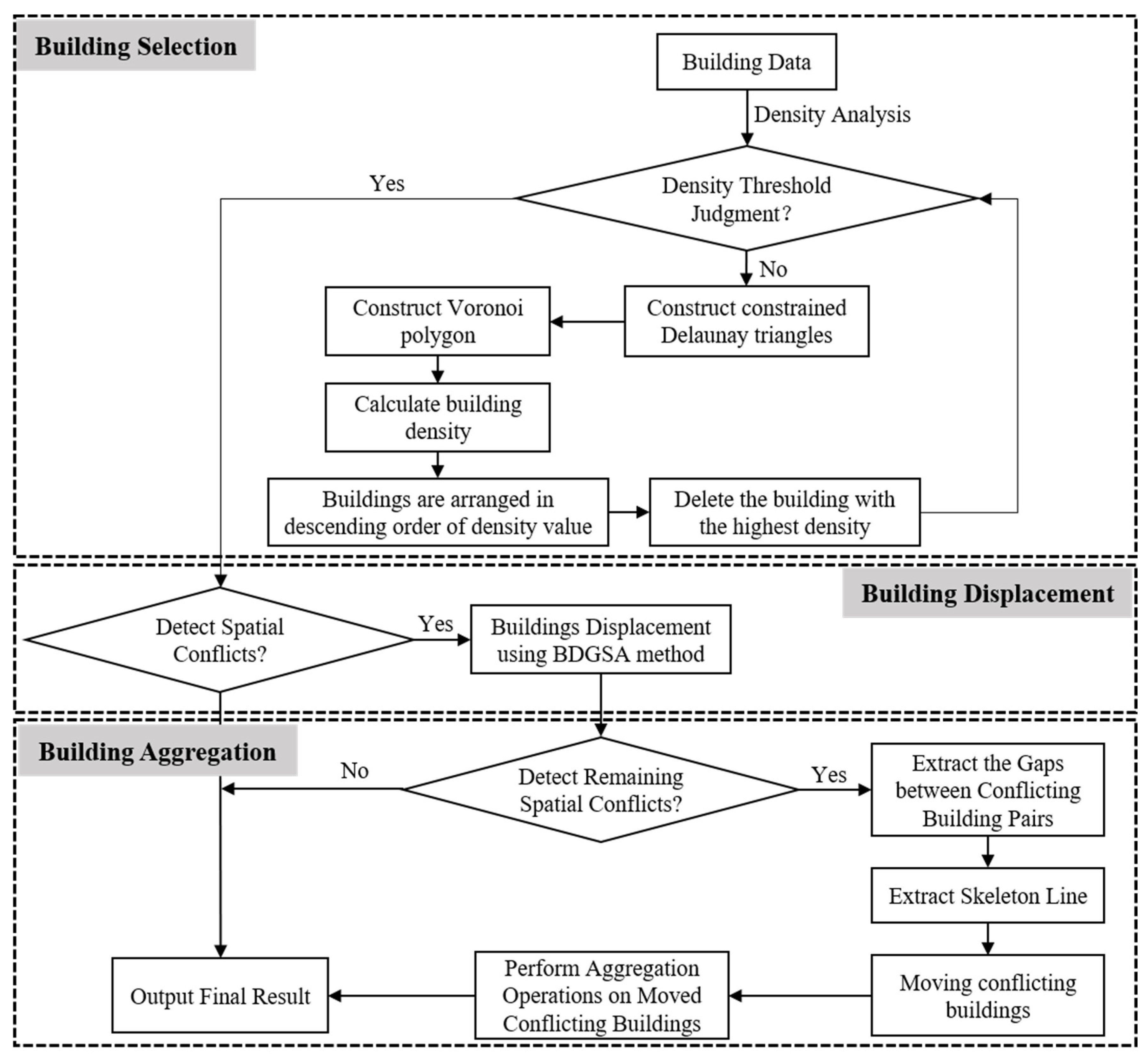
• A new heuristic framework for resolving spatial conflicts of building features that combines the three cartographic generalization operators of selection, displacement, and aggregation.
• An efficient and intelligent algorithm for displacing buildings in urban villages. This algorithm is called Building Displacement based on Genetic Simulated Annealing Algorithm (BDGSA), and can be used to solve spatial conflicts between buildings and other features.

The rest of this paper is organized as follows. Section 2 presents a review of previous work on feature displacement, mainly the displacement of buildings. Section 3 describes the core steps and details of the proposed algorithm. Section 4 details the experimental results and evaluations of the method. Section 5 discusses the results of the comparisons of the proposed approach with traditional methods. Section 6 presents the conclusions and some suggestions for future research.

2. Related Works

Different displacement methods have been proposed to resolve the spatial conflicts between buildings and other features. These approaches can be divided into two categories: mechanical methods and optimization methods.

Using mechanical methods, conflicting features move sequentially according to a pre-calculated displacement order. Mackaness [17] proposed a proportional radial displacement algorithm for point features, which considers the effect of distance attenuation. At the same time, the algorithm can be extended to include other data types by sensitizing linear and polygonal features. RUAS [18] presented a displacement method for buildings that considers multiple cartographic constraints and combines multiple cartographic generalization operators. Lonergan and Jones [19] proposed an iterative building displacement method, which improves the map quality measure and search strategy. Basaraner [20] proposed a zone-based iterative building displacement method that uses spatial analysis to detect conflicting buildings in the generalization zones, and then the displacement candidate and vector are decided by means of Voronoi tessellation, spatial analysis techniques and combined multiple criteria. Sahbaz and Basaraner [21] proposed a more practical method of zonal displacement for buildings. This method first creates building groups and zones through Voronoi tessellation and buffering, then grid points are generated and weighted through kernel density estimation and buffer analysis to find appropriate positions, and finally, visual assessment and quantitative analysis are employed to measure the displacement results. Chen and Qian [22] proposed a method for regularizing buildings by combining skeleton lines and Minkowski addition. In this method, the angular bisector method is used to dissipate conflicts among the redundant vertices in the building outlines. Generally, mechanical methods solve spatial conflicts from a local perspective and will repeatedly cause secondary conflicts.

Due to the limitations of mechanical methods, optimization methods have become the focus of research. In contrast to mechanical methods, optimization methods consider multiple conflicting objects and resolve spatial conflicts simultaneously. Optimization methods can be classified into two categories: functional optimization methods and combinational optimization methods.

Functional optimization methods establish mathematical equations by combining various cartographic constraints with models in the fields of material mechanics, mathematics, and physics, and then realize the displacement of features in map generalization. Højholt [23] proposed a method for displacement based on the finite element method (FEM). This method treats displacement as the deformation of an elastic body. Some scholars have presented displacement using least-squares adjustment (LSA). Among them, Harrie and Sarjakoski [24] constructed an overdetermined equation system using generalization constraints, solving it based on least-squares adjustment. The displacement process did not end until a desired degree of accuracy was reached through the conjugate gradient method. Sester [25] regarded displacement as an optimization problem, and thus, interior constraints and exterior constraints can be formulated in terms of a least-squares adjustment approach. Some studies applied displacement based on the beams model [26] and the snake algorithm [27]. However, as stated by Liu et al. [27], parameters in these approaches are difficult to determine and need to be identified using intelligent methods. From a global view, Ai et al. [16] presented an approach using a vector field and isoline model, which is effective in the maintenance of spatial relationships between buildings but may perform poorly in high-density areas. Maruyama et al. [28] addressed building displacement as a constrained optimization problem utilizing linear programming. They identified spatial relationships among map objects as constraints and optimized the cost function that penalizes the excessive displacement of buildings according to the map scale.

Combinatorial optimization methods directly use various combinatorial optimization algorithms to find an optimal solution among many candidate solutions. This kind of method has achieved satisfactory displacement effects. Ware and Jones [29] used steepest gradient descent (SGD) and simulated annealing (SA) approaches to reduce conflicts; the comparison results showed that the SA has a better ability to resolve spatial conflicts. Subsequently, Ware, Jones, and Thomas [30] improved this approach by taking generalization operations such as displacement, deletion, exaggeration, and reduction as candidates in the SA. Wilson, Ware, and Ware [31] used the genetic algorithm (GA) to realize the displacement of buildings and achieved a better displacement result. Sun et al. [32] proposed an immune genetic algorithm (IGA) that combines the self-adjustment of the individual concentration and the elite preservation methods with GA. Compared with the GA displacement results, IGA has satisfactory spatial conflict resolution results. Huang et al. [33] proposed an improved particle swarm optimization (PSO) algorithm for the displacement of buildings, which combines PSO with the cultural algorithm computational framework. These optimization algorithms all use a single population for evolution. To overcome the shortcomings of single-population evolution, Li et al. [34] proposed a building displacement method based on the multiple-population genetic algorithm (BDMPGA). This method uses an immigration operator to establish connections between the various populations to realize information exchange between various populations. The optimal displacement scheme is a result of the comprehensive evolution of multiple populations.

Through the literature summarized above, we can conclude the following: (1) Mechanical methods only use the displacement operation to displace features sequentially to resolve spatial conflicts. These kinds of methods are relatively simple and lack high intelligence. (2) Optimization methods, such as functional optimization methods and combinatorial optimization methods, use mathematical concepts and heuristic search strategies to obtain the best displacement scheme. However, traditional optimization algorithms such as GA and SA cannot resolve all possible spatial conflicts and even generate secondary conflicts.

This study focused on resolving spatial conflicts between buildings and other features in urban villages. Its novelty lies in the proposed heuristic spatial conflict resolution framework, which overcomes previous defects using only a single displacement operator to solve spatial conflicts but adopts three cartographic generalization operators sequentially. In addition, for the ideal displacement effect, we propose the BDGSA for displacing buildings after the selection operation, which improves the deficiencies of the traditional GA and SA. The results of our experiment demonstrate the potential of this approach for the resolution of spatial conflict.

3. Methodologies

When the displacement space around conflicting features is insufficient, it is unrealistic to resolve spatial conflicts between the features only through displacement operation. Therefore, this study exploited a heuristic spatial conflict resolution framework by combining multiple generalization operators. Thus, the spatial conflicts between buildings and other features (i.e., buildings and roads) in urban villages are resolved by sequentially applying the three generalization operators of selection, displacement, and aggregation. Figure 1 presents the proposed framework for spatial conflict resolution of buildings in urban villages. This paper details the main steps of the framework in the following sections.

3.1. Building Selection Operation

The first step of our framework is to perform a selection operation of original buildings in the urban villages. The purpose is to reduce the building density and maintain the building density distribution in the block. The key steps of the selection operation include two parts: calculation of building density and determination of the selection strategy.

Building distribution density draws on the idea of point cluster distribution density and is defined as the distribution space occupied by each building. Based on the idea of ‘spatial competition’ [16], it is believed that each building exists to obtain its own living space, and the result of competition between adjacent buildings is a division of the space. This idea is consistent with the Voronoi diagram of point features; thus, the Voronoi polygons formed by constructing the Voronoi diagram for buildings are used to define the distribution density of buildings. Ai and Zhang [35] proposed the specific process of constructing Voronoi-like polygons of buildings. Constrained Delaunay triangulation is a powerful tool for detecting spatial proximity between vector features. The Voronoi-like polygon constructed based on the constrained Delaunay triangulation comprehensively considers the geometric characteristics of a building, such as the shape, size, and orientation, so that the detected spatial distance is consistent with the principle of human spatial cognition. Employing Voronoi-like polygons of buildings, the density of buildings can be defined as the reciprocal of the area of the Voronoi-like polygon surrounding each building. If the buildings are sparsely distributed, the area of the corresponding Voronoi-like polygon is larger, which means that the living space is larger and the density value is smaller; otherwise, the density value is larger. Equation (1) details the specific calculation method:

$$Densit{y}_{poly\_i}=\frac{1}{VoronoiAre{a}_i}$$

(1)

where $Densit{y}_{poly\_i}$ represents the density of the $i\mathrm{th}$ building, and $VoronoiAre{a}_i$ represents the area of the Voronoi-like polygon corresponding to the $i$th building.

This study used the density of buildings in the block as the termination condition for selection, i.e., after selection, if the density of buildings is less than the given density threshold, then the selection operation is stopped. The basic idea of the building selection operation is as follows. First, the constrained Delaunay triangulation is constructed, as presented in Figure 2b. Then, the Voronoi-like polygon is constructed based on the constructed constrained Delaunay triangulation, as presented in Figure 2c. Next, the density of each building surrounded by a Voronoi-like polygon is calculated. Then, the building with the highest density value is selected for deletion. If the building has the highest density, the area of the Voronoi-like polygon corresponding to the building is the smallest, which means that this building is less important. Next, to ensure the spatial distribution of buildings, adjacent buildings are not deleted continuously, i.e., after each building is deleted, other buildings in the first-order neighborhood are not deleted, and the building with the highest density is identified from the remaining buildings and deleted. The space occupied by the deleted building is equally divided by other nearby buildings. Therefore, after each round of deletion operation is completed, the Voronoi polygon is reconstructed, its density is calculated for the remaining buildings, and the next round of deletion operation is performed. When the density of buildings in the block is less than a given density threshold $DensityT$, the selection operation is stopped. Figure 2d shows the result after the first round of the selection operation. The buildings that have been selected are shown in green. Figure 2e shows the result after the second round of the selection operation. The buildings that have been selected are shown in purple. Figure 2f shows the result after the third round of the selection operation. The buildings that have been selected are shown in cyan. The specific operation process is shown in Figure 2.

3.2. Building Displacement Operation

Our method first reduces the density of buildings by building selection operations and generates displacement spaces in each block. Then, the building displacement operation (i.e., BDGSA) is applied to resolve spatial conflicts for each building block separately. The following is a detailed introduction to the specific implementation of BDGSA from several aspects.

3.2.1. Population Initialization

BDGSA uses real number coding to generate chromosomes; specifically, the displacement distances of each building in the block in the X direction and Y direction are expressed as a chromosome. First, the displacement distance of each building in the X direction and the Y direction are randomly generated according to the determined maximum displacement range of the building. Then, the displacement distances of all the buildings in the block are spliced together to form a chromosome, which represents a candidate displacement scheme for the buildings in the block. Finally, randomly generated $N$ chromosomes form the initial population of BDGSA for subsequent evolution. Figure 3 shows a representation of one chromosome and one population.

3.2.2. Genetic Operations

The BDGSA consists of three genetic operations: chromosome selection, chromosome crossover and chromosome mutation. This study adopted the roulette selection method, the algorithmic crossover method, and the non-uniform mutation method, as detailed in this section.

The roulette selection method refers to the selection of an appropriate chromosome test strategy according to the chromosome’s fitness value. Assuming that the population size is $N$ and the fitness value of chromosome $X_i$ is $f_{X_i}$, the probability of chromosome $X_i$ being selected can be calculated using Equation (2).

$$P_{X_i}=f_{X_i}/{{\displaystyle \sum }}_{i=1}^N{f}_{X_i} \left(i=1,2,\dots ,N\right)$$

(2)

It can be seen from the selection formula that if the fitness value of a chromosome is higher, the probability of it being selected is also greater; conversely, a chromosome with a lower fitness value is less likely to be selected.

The algorithmic crossover method is a crossover strategy adapted to real number-coded chromosomes. Two new chromosomes are obtained through linear operations on two paired chromosomes. If the algorithmic crossover is performed between chromosome $X_i$ and chromosome $X_j$, the two new chromosomes, $X_i^{\prime }$ and $Y_j^{\prime }$, generated after the algorithmic crossover operation, can be calculated using Equation (3).

$$\{\begin{array}{c}{X}_i^{\prime }=\alpha \times X_i+\left(1-\alpha \right)\times X_j\\ Y_j^{\prime }=\alpha \times X_j+\left(1-\alpha \right)\times X_i\end{array}$$

(3)

When performing a non-uniform mutation operation on the $k$-th gene $x_{ik}$ of the $i$-th chromosome, the new gene value, $x_{ik}^{\prime }$, is determined using Equation (4).

$$x_{ik}^{\prime }=\{\begin{array}{c}{x}_{ik}+\left(x_{ik}-U_{max}^k\right)\times f\left(gen\right), r\ge 0.5\\ x_{ik}+\left(U_{min}^k-x_{ik}\right)\times f\left(gen\right), r<0.5\end{array}$$

(4)

where $U_{max}^k$ is the maximum value of the gene, and $U_{min}^k$ is the minimum value of the gene, $f\left(gen\right)=r_2\times {\left(1-gen/MaxGen\right)}^2$, where $r_2$ is a random number in the range of [0, 1] that meets the uniform probability distribution, $gen$ is the current iteration number. $MaxGen$ is the maximum iteration number, and $r$ represents a random number in the range of [0, 1].

3.2.3. Simulated Annealing Operation

The purpose of introducing the idea of SA into GA is to improve the local search ability of traditional GA and then to ensure that BDGSA has strong local and global search abilities. The specific operation is after the fitness value of the chromosome in the offspring population is calculated by the fitness function, and the fitness value of each chromosome in the offspring population is compared with the corresponding chromosome in the parent population. If the offspring chromosomes are better, replace the corresponding chromosomes in the parent population with offspring chromosomes; otherwise, Metropolis sampling stability criteria are used to determine whether to update the corresponding chromosomes in the parent population with new chromosomes in the offspring population [29].

3.2.4. Objective Function

The basic idea of BDGSA is to integrate SA in the evolution process of GA. Therefore, similarly to the construction of the objective function and fitness function of the GA, BDGSA also considers three constraints, namely the number of remaining conflicts between buildings and buildings, the number of remaining conflicts between buildings and roads, and the total displacement distance of all buildings. Specific definitions are presented subsequently.

Regarding the number of remaining conflicts between buildings and buildings, for two buildings, $B_i$ and $B_j$, $MinDist\left(B_i,B_j\right)$ is the minimum distance between buildings $B_i$ and $B_j$. $conf\left(B_i,B_j\right)$ represents a spatial conflict between buildings $B_i$ and $B_j$. If $MinDist\left(B_i,B_j\right)$ is less than the predefined distance threshold, $B{B}_{tol}$, then $conf\left(B_i,B_j\right)=1$; otherwise, $conf\left(B_i,B_j\right)=0$. Thus, the number of remaining conflicts between all buildings can be expressed as:

$$f_{BB\_conf}={{\displaystyle \sum }}_{i=1}^n{{\displaystyle \sum }}_{j=1}^{n}conf\left(B_i,B_j\right)$$

(5)

Regarding the number of remaining conflicts between buildings and roads, for building $B_i$ and road $R_j$, $MinDist\left(B_i,R_j\right)$ is the minimum distance between building $B_i$ and road $R_j$, and $conf\left(B_i,R_j\right)$ represents a spatial conflict between building $B_i$ and road $R_j$. If $MinDist\left(B_i,R_j\right)$ is less than the predefined distance threshold, $B{R}_{tol}$, then $conf\left(B_i,R_j\right)=1$; otherwise, $conf\left(B_i,R_j\right)=0$. Thus, the number of conflicts between buildings and roads can be expressed as:

$$f_{BR\_conf}={{\displaystyle \sum }}_{i=1}^n{{\displaystyle \sum }}_{j=1}^{m}conf\left(B_i,R_j\right)$$

(6)

The total displacement distance of all buildings is measured to evaluate the positional accuracy after displacement. The displacement must be within a certain range of the positional accuracy, and the smaller the total displacement distances are, the better the positional accuracy is maintained. The total displacement distances of all the buildings are calculated by summing the displacement distances in the X and Y directions of all the buildings. The expression is as follows:

$$f_{TotalDist}={{\displaystyle \sum }}_{i=1}^n\left(\sqrt{d{x}_i^2}+\sqrt{d{y}_i^2}\right)$$

(7)

Finally, the calculation formula of the objective function is as shown in Equation (8).

$$Min\left(f\right)=w_1\times f_{BB\_conf}+w_2\times f_{BR\_conf}+w_3\times f_{TotalDist}$$

(8)

where $w_1$, $w_2$ and $w_3$ are weights for $f_{BB\_conf}$, $f_{BR\_conf}$, and $f_{TotalDist}$, respectively. The weight-setting principle of the three parameters is as follows: $w_2>w_1>w_3$. The fitness function is obtained after the objective function undergoes a linear transformation. In this study, the reciprocal of the objective function value was taken as the fitness value, as shown in Equation (9).

$$MaxFitness=\frac{1}{Min\left(f\right)}$$

(9)

3.2.5. Algorithm Flow

The specific implementation process of the BDGSA is shown in Figure 4.

• Initialize control parameters: population size, $Nu{m}_p$, maximum number of iterations $MaxGen$, chromosome selection probability, $P_s$, crossover probability, $P_c$, mutation probability, $P_m$, annealing initial temperature, $T_0$, temperature cooling coefficient, $k$, and termination temperature, $T_{end}$.
• According to the coding method, randomly generate $Nu{m}_p$ chromosome s to form the initial population and use Equations (5) and (9) to calculate the fitness value, $f_i$, of each chromosome in the population, where $i=1,2,\dots ,N$.
• Set loop variable $gen=0$.
• Perform genetic operations on the population to generate a new offspring population and calculate the fitness value, $f_i^{\prime }$, of each chromosome in the offspring population.
• Perform simulated annealing operation on the chromosomes in the offspring population, i.e., the fitness value, $f_i^{\prime }$, of each chromosome in the offspring population is compared with the fitness value, $f_i$, of the corresponding chromosome in the parent population. If $f_i^{\prime }>f_i$, then replace the existing chromosome with the new chromosome. Otherwise, accept the new chromosome with probability $P=exp\left(\left(f_i-f_i^{\prime }\right)/T\right)$.
• If $gen<MaxGen$, increase the loop variable by 1, $gen=gen+1$, and return to step (4). Otherwise, transpose step (7).
• If the current temperature, $T_i$, is less than the end temperature, $T_{end}$, i.e., $T_i<T_{end}$, the algorithm ends and returns to the global optimal solution. Otherwise, the cooling operation is performed, i.e., $T_{i+1}=k\times T_i$, and transpose step (3).
• According to the returned global optimal solution, i.e., the amount of displacement in the $X$ direction and the amount of displacement amount in the $Y$ direction corresponding to each building, perform the displacement operation on the building to obtain the result of the displacement of the building.

3.3. Building Aggregation Operation

Due to the limited displacement space around conflicting buildings in urban villages, the displacement operation still cannot eliminate spatial conflicts between the buildings. Moreover, it is possible that secondary conflicts will occur in local high-density areas. At this point, the aggregation operation can be used to merge the conflicting building pairs into a whole to eliminate spatial conflicts between the buildings.

According to the spatial relationship between remaining conflict buildings, the conflicts are divided into three types: intersecting relationship, tangent relationship, and separation relationship. Among them, the spatial conflict between a building with an intersecting relationship and a tangent relationship refers to the spatial overwhelming conflict, which can be resolved using the ’aggregation’ tool within ArcGIS software. The spatial conflict between buildings with a separated relationship belongs to the spatial proximity conflict. For this type of spatial conflict, the conflicting buildings are first moved, and then aggregation is adopted to eliminate the spatial conflicts. The movement of conflicting buildings can squeeze out redundant blank gaps, thereby ensuring the balance of the building area of the entire block.

When moving conflicting buildings, two key parameters must be determined, namely the movement direction and the movement distance. For the movement direction, first construct a constrained Delaunay triangle network for the adjacent conflicting building pairs to obtain the visibility area. Then, extract the skeleton line of the visibility area by tracing each triangle, i.e., solid blue line in Figure 5. Finally, use least-squares multiplication to fit the extracted skeleton line, and take the normal direction of the fitted straight line as the movement direction of the conflicting building. For the movement distance, the area of conflicting buildings should be considered as the constraint condition. First, calculate the shortest distance between a pair of conflicting buildings. Then, determine the moving distance of conflicting buildings according to the area ratio. This method makes the conflicting buildings with large areas move a small distance, thus ensuring the position accuracy. The specific process is shown in Figure 5, where the red polygons represent the buildings after the movement.

4. Experiments and Evaluations

4.1. Experimental Data

In this experiment, the proposed method was used to deal with spatial conflicts between buildings and roads and between buildings and buildings in urban villages. The experimental data are shown in Figure 6. The experimental area was in the Chinese city of Guangzhou. The scale of the original data was 1:2000. There were 170 buildings in 4 blocks. The four blocks are marked with the numbers ①, ②, ③, and ④. It can be seen from Figure 6a that the density of buildings in each block is relatively high. When the road was widened, there were many spatial overlaps and proximity conflicts between the objects. The experimental framework was implemented by using ArcGIS 10.2 software assisted by MATLAB 2022a.

4.2. Setting Parameters

Before the algorithm runs, the parameter values need to be set. Reasonable parameter values have a significant impact on the results of the algorithm. The relevant parameters involved in this algorithm are as follows: the selection density threshold, $DensityT$, the conflict distance threshold between buildings, $B{B}_{tol}$, the conflict distance threshold between buildings and roads, $B{R}_{tol}$, population size, $Nu{m}_p$, the maximum number of iterations, $MaxGen$, selection probability, $P_s$, crossover probability, $P_c$, mutation probability, $P_m$, initial temperature, $T_0$, cooling rate, $k$, termination temperature, $T_{end}$, the weights of each index in the objective function, $w_1$, $w_2$, and $w_3$.

The building selection density, $DensityT$, was the empirical value obtained after many experiments. In this study, $DensityT=0.6$ was used as the building selection density threshold, i.e., when the density of buildings in the block was less than 0.6, the selection operation was stopped. The conflict distance threshold between buildings, $B{B}_{tol}$, was determined according to the scale with clear and legible constraints. Generally, the minimum distance threshold between objects is required to be 0.2 mm according to the graphic limits used in cartography; therefore, the conflict distance threshold between buildings was determined in this experiment to be $B{B}_{tol}=0.4$ m. The conflict distance threshold between a building and a road, $B{R}_{tol}$, was determined by three factors: scale, legibility constraints, and the value of road widening. The finally determined conflict distance threshold between buildings and roads was $B{R}_{tol}=0.9$ m.

Population size, $Nu{m}_p$, refers to the number of chromosomes contained in the population. If the value of the parameter $Nu{m}_p$ is small, the population will contain fewer chromosomes, which will shorten the running time of DBGSA, but may also lead to insufficient evolution and an inability to find the optimal solution. If the parameter $Nu{m}_p$ takes a larger value, it will increase the computational cost of the algorithm and reduce the computational efficiency. Wilson, Ware, and Ware [31] used heuristic experiments to determine that there is a certain linear proportional relationship between the reasonable value of the parameter $Nu{m}_p$ and the number of spatial conflicts in a block, $C$, as detailed in Equation (10).

$$Nu{m}_p=4\times C$$

(10)

The maximum number of iterations, $MaxGen$, is the judgement condition for the termination of the algorithm. Setting a larger $MaxGen$ parameter can obtain a more accurate optimal solution, but it will also increase the computational cost of the algorithm. At the same time, as the iteration progresses, the improvement range of the optimal solution will become smaller and smaller. Wilson, Ware, and Ware [31] used heuristic experiments to summarize the empirical formula between the maximum number of iterations, $MaxGen$, and the number of buildings in a block, $S$, as shown in Equation (11).

$$MaxGen=15\times S$$

(11)

In the BDGSA, the crossover operation is used to generate new individuals; thus, the crossover probability, $P_c$, should generally be a larger value. Scholars suggest that the value range of $P_c$ is [0.7, 0.9] [36]. To compare with the standard GA [31], the value of $P_c$ in this experiment was 0.8. The mutation operation is also a method for generating new individuals, and its frequency is controlled by the mutation probability, $P_m$. Scholars suggest that the value range of mutation probability, $P_m$, is [0.001, 0.05] [36]. To compare with the standard GA [31], the value of $P_m$ in the experiment was 0.008.

The initial temperature, $T_0$, the temperature cooling coefficient, $k$, and the end temperature, $T_{end}$, are the three parameters involved in the simulated annealing operation. Experiments show that the greater the initial temperature, the greater the probability of obtaining the optimal solution, but the time spent will also increase. Similarly, the smaller the temperature cooling coefficient, the slower the cooling, and although better optimization results will be obtained, it will increase the running time of the algorithm. Therefore, comprehensively considering the optimization quality and optimization efficiency, the values of the three parameters were determined using the empirical formula: initial temperature $T_0=3$, cooling rate $k=0.1$, and termination temperature $T_{end}=1$.

Due to the small distance between objects in urban villages, there is a certain spatial conflict in itself. Additionally, road widening operations will aggravate the spatial conflict between roads and buildings. The principle of displacement is to maintain the position accuracy of the objects as much as possible on the premise of resolving all spatial conflicts. Therefore, the weight values in the objective function in this algorithm are as follows: $w_1=50$, $w_2=100$, and $w_3=1$. To facilitate the comparison of experimental results, the weight of the objective function in the standard GA was also the same.

4.3. Spatial Conflict Detection

In this study, the constructed constrained Delaunay triangulation and the extracted skeleton lines were used to detect the conflict area between the objects. The detection result is shown in Figure 7, where Figure 7a shows the constructed constrained Delaunay triangulation and the extracted skeleton line in the gap space between the objects, which is represented by solid red line. The red area in Figure 7b represents the conflict area between the detected objects.

It can be seen from the detected result that due to the crowded buildings in blocks, the distances between buildings and between buildings and roads are small, which cannot meet the requirements of cartographic constraints. In particular, the spatial conflict between buildings and roads is more serious, which affects the correct expression of the spatial relationship between the objects.

4.4. Experimental Results and Evaluation of the Building Selection Operation

The results of building selection in each block are shown in Figure 8. From the results, it can be observed that the proposed selection method effectively selected important buildings, reduced the density of buildings, and maintained the distribution of buildings in the block. The selection results at different densities could be obtained according to the density threshold. Therefore, this selection method is suitable for multi-scale applications.

Table 1. Statistical information before and after the selection operation of each block.

Block ID	Before Selection				After Selection
	Number of Buildings	Block Density	<B-B> Number of Conflicts	<B-R> Number of Conflicts	Number of Buildings	Block Density	<B-B> Number of Conflicts	<B-R> Number of Conflicts
➀	20	0.74	0	13	13	0.57	0	10
➁	40	0.71	9	14	26	0.56	6	7
➂	69	0.71	23	28	48	0.57	15	17
➃	41	0.80	20	24	28	0.62	8	17
	170	—	52	79	115	—	29	51

shows the statistical information before and after the selection of each block. It can be seen from the statistical information that the total number of buildings after the selection operation is reduced to 68% of the original data, and the reduction in building density in each block is basically the same, which provides extra space for subsequent displacement operation. Due to the reduction in the number of buildings, certain spatial conflicts have been eliminated, and the number of spatial conflicts has been reduced from 131 to 80.

To determine the visualization effect of the building selection results, a linear relationship was established between the building density and the grey value. Figure 9a presents a grayscale image of the building before the selection; Figure 9b shows a grayscale image of the building after the selection. It can be seen from the figure that the grey distribution of the corresponding regions before and after the selection is roughly the same.

Figure 10 shows the result of spatial conflict detection on selected buildings. Figure 10a is the constructed constraint Delaunay triangulation (i.e., gray triangles) and the extracted skeleton line of the gap space (i.e., solid red line). Figure 10b shows the detected spatial conflict area, which are represented in red. Compared with the spatial conflict detection results before the building selection operation, some spatial conflicts have been eliminated.

4.5. Experimental Results and Evaluation of the Building Displacement Operation

Figure 11a shows the experimental results of using the BDGSA to displace the buildings in each block; Figure 11b shows the superimposed effect of the BDGSA displacement results and the original building data. The blue-outlined polygons represent the buildings after displacement, and the grey polygons represent the buildings before displacement.

Table 2. Statistical information of the BDGSA displacement results.

Block ID	Number of Buildings	Before Displacement		MaxGen	Nump	After Displacement		Total Displacement Distance (m)
		<B-B> Number of Conflicts	<B-R> Number of Conflicts			<B-B> Number of Conflicts	<B-B> Number of Conflicts
➀	13	0	10	11 × 195	40	0	0	3.606
➁	26	6	7	11 × 390	52	2	0	4.566
➂	48	15	17	11 × 720	128	3	1	6.441
➃	28	8	17	11 × 420	100	4	0	6.282
	115	29	51	—	—	9	1	20.895

details the statistical information of the BDGSA displacement results, including the number of spatial conflicts between buildings before and after the displacement, the number of spatial conflicts between buildings and roads, and the total displacement distance of buildings in each block. The statistical information can be utilized to evaluate the displacement effect of the BDGSA.

To better illustrate the displacement results of the BDGSA, we selected some examples of residual conflicts between buildings in each block, which are marked with black circles A-I in Figure 11. Figure 12 shows the detailed information of examples of residual conflicts, which the blue polygons represent the buildings after displacement. Statistical analysis revealed that there were three main spatial relationships between the remaining conflict objects: separation, tangency, and intersection. Figure 12A–C show the remaining conflict types with detached relationships; Figure 12D–F show the remaining conflict types with tangent relationships; and Figure 12G–I show the remaining conflict types with intersecting relationships. Spatial conflicts with detached relationships belong to spatial proximity conflicts, while spatial conflicts with tangent and intersecting relationships belong to spatial overlap conflicts.

4.6. Experimental Results and Evaluation of the Building Aggregation Operation

The aggregation operation was used to resolve the remaining spatial conflicts in this study. The steps used to achieve the aggregation operation were also different according to the type of spatial conflict; there was excess space between conflicting buildings with separate relationships. To maintain balance in the area of the buildings in the block, the conflicting building pairs were moved first and then aggregated. Figure 13 shows the movement effect of conflicting building pairs before they are aggregated, which red polygons represent the buildings after displacement and blue lines represent the extracted skeleton lines. The movement squeezed out any excess space between the conflicting building pairs.

Figure 14 shows the effect of first moving and then aggregating the remaining spatial conflicts with separate relationships in each block, and the effect of directly using the aggregation operation within ArcGIS software for the remaining spatial conflicts with tangent and intersecting relationships. In comparison with the result after displacement, it was found that after the aggregation operation, the remaining spatial conflicts between buildings in each block were all resolved.

5. Discussion

To better evaluate the spatial conflict resolution ability of the BDGSA proposed in this study, we implemented two other intelligent optimization algorithms to perform comparative experiments. Because the BDGSA incorporates the idea of SA into the traditional GA, the first comparative method is the standard GA, which was used by Wilson [31] to displace buildings. The other comparative method is the SA, which was proposed by Ware [29] to reduce conflicts. The experimental results of the BDGSA, GA, and SA are compared from the two aspects of the legibility constraint and the positional accuracy constraint. The legibility constraint uses the number of remaining spatial conflicts as the evaluation index, which indicates the ability of the algorithm to resolve spatial conflicts. The smaller this value is, the stronger the ability of the algorithm to resolve spatial conflicts is. The positional accuracy constraint uses the total displacement distance of all buildings as the evaluation index, which indicates the disruption degree of the positional accuracy. The smaller the value is, the better the positional accuracy is.

Figure 15a shows the displacement results based on the standard GA; Figure 15b shows the overlay display effect before and after building displacement using the GA. In the figure, the cyan-outlined polygons represent the displaced buildings using GA, and the gray polygons represent the buildings before displacement. The black circles A-I represent some examples of residual conflicts, which correspond to the one in Figure 11. The basic statistical information of the displacement results based on the GA is listed in

Table 3. Statistical information of the GA displacement results.

Block ID	Number of Buildings	Before Displacement		MaxGen	Nump	After Displacement		Total Displacement Distance (m)
		<B-B> Number of Conflicts	<B-R> Number of Conflicts			<B-B> Number of Conflicts	<B-B> Number of Conflicts
➀	13	0	10	195	40	0	0	5.621
➁	26	6	7	390	52	3	1	5.277
➂	48	15	17	720	128	3	1	10.272
➃	28	8	17	420	100	5	0	7.804
	115	29	51	—	—	11	2	28.974

. From Table 3, it can be seen that the GA cannot resolve all the spatial conflicts between buildings and other features. In particular, all spatial conflicts have been resolved in block 1. There are three unresolved spatial conflicts between buildings and buildings and one spatial conflict between buildings and roads in block 2. The number and type of remaining spatial conflicts in block 3 are the same as those in block 2. There are five unresolved spatial conflicts between buildings in block 4.

Figure 16a shows the displacement results based on SA; Figure 16b shows the overlay display effect before and after building displacement using SA. In the figure, the pink-outlined polygons represent the displaced buildings using SA; the grey polygons represent the buildings before the displacement. The black circles A-I represent some examples of residual conflicts, which correspond to the one in Figure 11. The basic statistical information of the displacement results based on the SA is listed in

Table 4. Statistical information of the SA displacement results.

Block ID	Number of Buildings	Before Displacement		Number of Cooling	After Displacement		Total Displacement Distance (m)
		<B-B> Number of Conflicts	<B-R> Number of Conflicts		<B-B> Number of Conflicts	<B-R> Number of Conflicts
➀	13	0	10	50	0	0	10.000
➁	26	6	7	50	1	0	22.000
➂	48	15	17	50	0	0	38.667
➃	28	8	17	50	3	0	24.667
	115	29	51	—	4	0	95.334

. Table 4 shows that the SA had one unresolved spatial conflict between buildings located in block 2.

Although these methods can be used to displace buildings and resolve spatial conflicts, they yield different displacement results. The statistical information above indicates the following:

• For the legibility constraint, the total numbers of remaining spatial conflicts after building displacement using the BDGSA, GA, and SA are 10, 13, and 4, respectively, and the proportions of conflict resolution are 87.5%, 83.75%, and 95%, respectively. Therefore, in terms of the ability to resolve spatial conflicts independently, SA is the best, followed by the BDGSA. The reason for this situation is that the objective function of the BDGSA is constructed with the number of spatial conflicts and the total displacement distance as constraints, whereas the objective function of SA is constructed only with the number of spatial conflicts as a constraint. The different constraints considered in the objective function led to the much larger displacement distance of SA than that of the BDGSA.
• For the positional accuracy constraint, the total displacement distances of the BDGSA, GA and SA are 20.895 m, 28.974 m, and 95.334 m, respectively. It can be seen from the statistical information that the total displacement distance of the BDGSA proposed in this study is the shortest, while the total displacement distance of SA is the largest. Therefore, the proposed BDGSA can better maintain the positional accuracy constraints of the displaced buildings, while the SA cannot.

Therefore, considering the two constraints of legibility constraint and positional accuracy constraint, the BDGSA achieves a better displacement effect. The main reason is that BDGSA introduces the idea of SA into the traditional GA and realizes the complementary advantages of GA and SA. BDGSA has strong local research ability and global search ability. Therefore, as the experimental results show, compared with GA and SA, BDGSA has a stronger comprehensive ability to solve spatial conflicts.

Successful displacement should not only solve all possible spatial conflicts after displacing some buildings but also ensure the positional accuracy of the displaced buildings. To better demonstrate the difference between the proposed BDGSA and the other two comparative methods in maintaining the positional accuracy of displaced buildings, we calculated the detailed statistical information, and the relevant statistical indicators of the building displacement distances in each block of the three methods of BDGSA, GA, and SA, as shown in

Table 5. Statistical information of the BDGSA displacement distance.

Block ID	Number of Buildings	Displacement Distance (m)
		Minimum	Maximum	Sum	Average	Standard Deviation
➀	13	0.000	0.886	3.606	0.277	0.259
➁	26	0.000	0.561	4.566	0.176	0.214
➂	48	0.000	0.492	6.441	0.134	0.168
➃	28	0.000	0.752	6.282	0.224	0.214

,

Table 6. Statistical information of the GA displacement distance.

Block ID	Number of Buildings	Displacement Distance (m)
		Minimum	Maximum	Sum	Average	Standard Deviation
➀	13	0.009	0.800	5.621	0.432	0.282
➁	26	0.009	0.558	5.277	0.203	0.192
➂	48	0.010	0.828	10.272	0.214	0.191
➃	28	0.019	0.694	7.804	0.279	0.211

and

Table 7. Statistical information of the SA displacement distance.

Block ID	Number of Buildings	Displacement Distance (m)
		Minimum	Maximum	Sum	Average	Standard Deviation
➀	13	0.333	1.000	10.000	0.769	0.274
➁	26	0.333	1.000	22.000	0.846	0.190
➂	48	0.333	1.000	38.667	0.806	0.224
➃	28	0.333	1.000	24.667	0.881	0.203

, which indicate the following:

• The statistical information that the minimum amount of displacement of buildings using the BDGSA in each block is 0.000 m, while the minimum displacements of the GA and SA are greater than 0 m. This suggests that if some buildings in the BDGSA do not conflict with any neighboring objects, they will not be moved to maintain position accuracy. If the area of a conflicting building is larger, it indicates that the building is relatively important, and its location accuracy should be ensured as much as possible without displacement.
• The average displacement distance of buildings in each block of the BDGSA is smaller than the corresponding blocks of the GA and SA, which shows that the BDGSA displacement method has a shorter displacement distance. Compared with the BDGSA and GA, the SA exhibits the largest average displacement value in each block, which shows that the SA is weak in maintaining the accuracy of the building displacement. The main reason is that SA tries to designate displacement candidate positions in a continuous displacement space; therefore, the size of the displacement distance is greatly affected by the subsequent positions.

To objectively evaluate the maintenance of the building’s relative position, this study compares the changes in the area of Voronoi polygons before and after building displacement. The Voronoi polygon of one building represents its competition with the surrounding space. When the relative position between adjacent buildings changes, the size of the corresponding Voronoi polygons will also change. Therefore, by analyzing the size of changes in Voronoi polygons before and after buildings displacement, the effect of maintaining the spatial distribution and relative positional relationship of each building can be quantitatively evaluated. Figure 17a depicts the Voronoi polygons of the buildings in each block before the displacement, i.e., red polygons, and Figure 17b is the Voronoi polygons of buildings in each block after the displacement, i.e., red polygons. Visual observation revealed that the Voronoi polygons of the buildings before and after the displacement are very similar in structure. This indicates that the BDGSA can sufficiently maintain the spatial distribution of buildings after displacement.

For quantitative analysis, Figure 18 presents the areas of Voronoi polygons before and after the displacement of the buildings of block ①, block ②, block ③, and block ④. The abscissa represents the area of the Voronoi polygon of the building before the displacement; the ordinate represents the area of the Voronoi polygon of the building after the displacement. The correlation coefficients, R², of each block are 0.8623, 0.9747, 0.9771, and 0.9744, indicating that the area of the Voronoi polygons before and after the building displacement is highly correlated. The quantitative analysis results show that the displacement operation can adequately maintain the spatial distribution and relative position of the building after displacement.

6. Conclusions

Generalizing building data at different scales plays an important role in the application of network map services, automatic drive, and urban planning. In these applications, map generalization approaches are widely used to abstract the geometric representations of building data. However, due to the reduction in map scale or the application of related generalization operators, spatial conflicts will inevitably be generated between buildings and between buildings and other features, especially in blocks with high building density. Traditional approaches mainly adopt displacement operations to resolve spatial conflicts between features. The experiments showed that when there is no redundant displacement space around the conflicting buildings, spatial conflicts cannot be resolved using only the displacement operation, except with other generalization operators. In this sense, this research has presented a heuristic spatial conflict resolution framework combining the three cartographic generalization operators of selection, displacement, and aggregation. This solution was effective for our cases because the building density in urban villages is very high, which provides a new way to solve spatial conflict between buildings and other features during map generalization.

For the core displacement operation, we have proposed a new BDGSA based on the combinatorial optimization concept. This displacement method combines the advantages of the traditional GA and SA and has a stronger spatial conflict resolution ability. We evaluated the proposed approach with high-density block data derived from Guangzhou topographic datasets. The experimental results demonstrate the feasibility of the proposed approach from both qualitative and quantitative aspects, indicating that this research has strong theoretical significance and practical application value.

The heuristic framework proposed in this study sequentially adopted three cartographic generalization operators. The application order of the three cartographic generalization operators was fixed. For high-density blocks in urban villages, the sequential use of three cartographic generalization operators can solve the spatial conflicts between building features and other features. However, the sequential use of the three cartographic generalization operators also has some shortcomings. In practice, it is necessary to select the optimal application order of the generalization operators according to the specific spatial conflict types and conflict features. Future work will combine relevant models in machine learning and other fields to study the optimal application order of generalization operators. At the same time, the framework only combined three cartographic operators: selection, displacement, and aggregation. However, if the density of buildings in the test area meets the requirements, it is not necessary to reduce the density through the selection operator. Therefore, it is necessary to adopt other generalization operators according to different spatial conflict types and different conflict features to resolve spatial conflicts, such as the typification operator. Follow-up research will explore the combination of more generalization operators to resolve more complex types of spatial conflicts.

References

1. Yang, M.; Yuan, T.; Yan, X.; Ai, T.; Jiang, C. A hybrid approach to building simplification with an evaluator from a backpropagation neural network. Int. J. Geogr. Inf. Sci. 2022, 36, 280–309. [Google Scholar] [CrossRef]
2. Zhou, Z.; Fu, C.; Weibel, R. Move and remove: Multi-task learning for building simplification in vector maps with a graph convolutional neural network. ISPRS J. Photogamm. Remote Sens. 2023, 202, 205–218. [Google Scholar] [CrossRef]
3. Karsznia, I.; Weibel, R. Improving settlement selection for small-scale maps using data enrichment and machine learning. Cartogr. Geogr. Inf. Sci. 2018, 45, 111–127. [Google Scholar] [CrossRef]
4. Wang, X.; Burghardt, D. A typification method for linear building groups based on stroke simplification. Geocarto Int. 2021, 36, 1732–1751. [Google Scholar] [CrossRef]
5. Gong, X.; Wu, F. A typification method for linear pattern in urban building generalisation. Geocarto Int. 2018, 33, 189–207. [Google Scholar] [CrossRef]
6. Burghardt, D.; Cecconi, A. Mesh simplification for building typification. Int. J. Geogr. Inf. Sci. 2007, 21, 283–298. [Google Scholar] [CrossRef]
7. Yu, W.; Zhang, Y.; Chen, Z.; Ai, T. Sparse reconstruction with spatial structures to automatically determine neighbors. Int. J. Geogr. Inf. Sci. 2022, 36, 338–359. [Google Scholar] [CrossRef]
8. Yan, X.; Ai, T.; Yang, M.; Yin, H. A graph convolutional neural network for classification of building patterns using spatial vector data. ISPRS J. Photogamm. Remote Sens. 2019, 150, 259–273. [Google Scholar] [CrossRef]
9. He, X.; Zhang, X.; Xin, Q. Recognition of building group patterns in topographic maps based on graph partitioning and random forest. ISPRS J. Photogamm. Remote Sens. 2018, 136, 26–40. [Google Scholar] [CrossRef]
10. Staněk, K.; Šilhák, P.; Ryglová, A. A graphical generalization of localized morphological discontinuities on medium-scale state topographic maps. J. Geovisualization Spat. Anal. 2022, 6, 20. [Google Scholar] [CrossRef]
11. Harrie, L.; Oucheikh, R.; Nilsson, Å.; Oxenstierna, A.; Cederholm, P.; Wei, L.; Richter, K.-F.; Olsson, P. Label placement challenges in city wayfinding map production—Identification and possible solutions. J. Geovisualization Spat. Anal. 2022, 6, 16. [Google Scholar] [CrossRef]
12. Pilehforooshha, P.; Karimi, M.; Mansourian, A. A new model combining building block displacement and building block area reduction for resolving spatial conflicts. Trans. GIS 2021, 25, 1366–1395. [Google Scholar] [CrossRef]
13. Ai, T.; Yin, H.; Shen, Y.; Yang, M.; Wang, L. A formal model of neighborhood representation and applications in urban building aggregation supported by Delaunay triangulation. PLoS ONE 2019, 14, e0218877. [Google Scholar] [CrossRef] [PubMed]
14. Guo, Q.; Li, G.; Wang, Y.; Liu, J.; Wei, Z. The method of progressive typification for building groups with straight linear patterns. Acta Geodaetica Cartogr. Sin. 2020, 49, 1354–1364. [Google Scholar] [CrossRef]
15. Wei, Z.; He, J.; Wang, L.; Wang, Y.; Guo, Q. A collaborative displacement approach for spatial conflicts in urban building map generalization. IEEE Access 2018, 6, 26918–26929. [Google Scholar] [CrossRef]
16. Ai, T.; Zhang, X.; Zhou, Q.; Yang, M. A vector field model to handle the displacement of multiple conflicts in building generalization. Int. J. Geogr. Inf. Sci. 2015, 29, 1310–1331. [Google Scholar] [CrossRef]
17. Mackaness, W.A. An algorithm for conflict identification and feature displacement in automated map generalization. Cartogr. Geogr. Inf. Sci. 1994, 21, 219–232. [Google Scholar] [CrossRef]
18. RUAS, A. A method for building displacement in automated map generalisation. Int. J. Geogr. Inf. Sci. 1998, 12, 789–803. [Google Scholar] [CrossRef]
19. Lonergan, M.; Jones, C.B. An iterative displacement method for conflict resolution in map generalization. Algorithmica 2001, 30, 287–301. [Google Scholar] [CrossRef]
20. Basaraner, M. A zone-based iterative building displacement method through the collective use of Voronoi Tessellation, spatial analysis and multicriteria decision making. Bol. Ciênc. Geod. 2011, 17, 161–187. [Google Scholar] [CrossRef]
21. Sahbaz, K.; Basaraner, M. A zonal displacement approach via grid point weighting in building generalization. ISPRS Int. J. Geo-Inf. 2021, 10, 105. [Google Scholar] [CrossRef]
22. Chen, G.; Qian, H. A method for regularizing buildings through combining skeleton lines and minkowski addition. ISPRS Int. J. Geo-Inf. 2023, 12, 363. [Google Scholar] [CrossRef]
23. Højholt, P. Solving space conflicts in map generalization: Using a finite element method. Cartogr. Geogr. Inf. Sci. 2000, 27, 65–74. [Google Scholar] [CrossRef]
24. Harrie, L.; Sarjakoski, T. Simultaneous graphic generalization of vector data sets. GeoInformatica 2002, 6, 233–261. [Google Scholar] [CrossRef]
25. Sester, M. Optimization approaches for generalization and data abstraction. Int. J. Geogr. Inf. Sci. 2005, 19, 871–897. [Google Scholar] [CrossRef]
26. Bader, M.; Barrault, M.; Weibel, R. Building displacement over a ductile truss. Int. J. Geogr. Inf. Sci. 2005, 19, 915–936. [Google Scholar] [CrossRef]
27. Liu, Y.; Guo, Q.; Sun, Y.; Ma, X. A combined approach to cartographic displacement for buildings based on skeleton and improved elastic beam algorithm. PLoS ONE 2014, 9, e113953. [Google Scholar] [CrossRef]
28. Maruyama, K.; Takahashi, S.; Wu, H.; Misue, K.; Arikawa, M. Scale-Aware cartographic displacement based on constrained optimization. In Proceedings of the 2019 23rd International Conference Information Visualisation (IV), Paris, France, 2–5 July 2019; pp. 74–80. [Google Scholar] [CrossRef]
29. Ware, J.M.; Jones, C.B. Conflict reduction in map generalization using iterative improvement. GeoInformatica 1998, 2, 383–407. [Google Scholar] [CrossRef]
30. Ware, J.M.; Jones, C.B.; Thomas, N. Automated map generalization with multiple operators: A simulated annealing approach. Int. J. Geogr. Inf. Sci. 2003, 17, 743–769. [Google Scholar] [CrossRef]
31. Wilson, I.D.; Ware, J.M.; Ware, J.A. A Genetic Algorithm approach to cartographic map generalisation. Comput. Ind. 2003, 52, 291–304. [Google Scholar] [CrossRef]
32. Sun, Y.; Guo, Q.; Liu, Y.; Ma, X.; Weng, J. An immune genetic algorithm to buildings displacement in cartographic generalization. Trans. GIS 2016, 20, 585–612. [Google Scholar] [CrossRef]
33. Huang, H.; Guo, Q.; Sun, Y.; Liu, Y. Reducing building conflicts in map generalization with an improved PSO algorithm. ISPRS Int. J. Geo-Inf. 2017, 6, 127. [Google Scholar] [CrossRef]
34. Li, W.; Ai, T.; Shen, Y.; Yang, W.; Wang, W. A novel method for building displacement based on multipopulation genetic algorithm. Appl. Sci. 2020, 10, 8441. [Google Scholar] [CrossRef]
35. Ai, T.; Zhang, X. The aggregation of urban building clusters based on the skeleton partitioning of gap space. In The European Information Society; Fabrikant, S.I., Wachowicz, M., Eds.; Springer: Berlin/Heidelberg, Germany, 2007; pp. 153–170. [Google Scholar]
36. Schaffer, J.D.; Caruana, R.A.; Eshelman, L.J.; Das, R. A study of control parameters affecting online performance of genetic algorithms for function optimization. In Proceedings of the Third International Conference on Genetic Algorithms; Morgan Kaufmann Publishers Inc.: San Francisco, CA, USA, 1989; pp. 51–60. [Google Scholar]
Figure 1. The framework for the spatial conflict resolution of buildings in urban villages.
Ijgi 12 00392 g001
Figure 2. Schematic diagram of building selection operation to maintain spatial distribution: (a) experimental data; (b) the result of constrained Delaunay triangulation construction; (c) the result of Voronoi-like polygon construction; (d) the result after the first round of the selection operation; (e) the result after the second round of the selection operation; (f) the result after the third round of the selection operation.
Ijgi 12 00392 g002
Figure 3. Representation of one chromosome and one population: (a) one chromosome, B i ( i = 1 , 2 , , n ) represents the displacement distance of the i th building in the X and Y directions; (b) one population, C j ( i = 1 , 2 , , m ) represents the j th chromosome in a population.
Ijgi 12 00392 g003
Figure 4. Buildings displacement operation using the BDGSA.
Ijgi 12 00392 g004
Figure 5. The aggregation operation of conflicting building pairs: (a) the result of not considering the area factor; (b) the result of considering the area factor.
Ijgi 12 00392 g005
Figure 6. Experimental data: (a) original data; (b) results after road widening.
Ijgi 12 00392 g006
Figure 7. Result of the detected spatial conflict: (a) constructed constrained Delaunay triangulation and extracted skeleton lines; (b) detected spatial conflict area.
Ijgi 12 00392 g007
Figure 8. Comparison of results before and after the building selection operation: (a) building before selection operation; (b) building after selection operation.
Ijgi 12 00392 g008
Figure 9. Grayscale comparison of building density before and after selection: (a) grayscale image of the building before the selection; (b) grayscale image of the building after the selection.
Ijgi 12 00392 g009
Figure 10. The spatial conflict detection results after the building selection operation: (a) constructed constrained Delaunay triangulation and extracted skeleton lines; (b) detected spatial conflict area.
Ijgi 12 00392 g010
Figure 11. Experimental results of the BDGSA: (a) displacement result of the BDGSA; (b) results of the overlay with the buildings before displacement.
Ijgi 12 00392 g011
Figure 12. Remaining spatial conflict types after the displacement operation using the BDGSA.
Ijgi 12 00392 g012
Figure 13. Movement effect of the conflicting building pairs before aggregation: (a) movement effect of the conflicting building pairs with tangent relationships; (b,c) movement effect of the conflicting building pairs with detached relationships.
Ijgi 12 00392 g013
Figure 14. Result after the aggregation operation: (a) the aggregate result of the remaining spatial conflict examples; (b) final experimental result.
Ijgi 12 00392 g014
Figure 15. Experimental results of the GA: (a) displacement results of GA; (b) results of the overlay with the buildings before displacement.
Ijgi 12 00392 g015
Figure 16. Experimental results of SA: (a) displacement results of SA; (b) results of the overlay with buildings before displacement.
Ijgi 12 00392 g016
Figure 17. Voronoi polygons of buildings before and after the displacement: (a) Voronoi polygons of buildings before the displacement; (b) Voronoi polygons of buildings after the displacement.
Ijgi 12 00392 g017
Figure 18. Relationship between the areas of the Voronoi polygons of buildings before and after displacement: (a) relationship between the areas of the Voronoi polygons of buildings before and after displacement of block ①; (b) relationship between the areas of the Voronoi polygons of buildings before and after displacement of block ②; (c) relationship between the areas of the Voronoi polygons of buildings before and after displacement of block ③; (d) relationship between the areas of the Voronoi polygons of buildings before and after displacement of block ④.
Ijgi 12 00392 g018