Explanatory Factors of Daily Mobility Patterns in Suburban Areas: Applications and Taxonomy of Two Metropolitan Corridors in Madrid Region

Abstract

Understanding the characteristics that shape mobility could help to achieve more sustainable transport systems. A considerable body of scientific studies tries to determine these characteristics at the urban level. However, there is a lack of studies analyzing those factors for the heterogeneous zones existing in the suburbs of big cities. The study presented in this paper intends to fill this gap, in the context of two metropolitan corridors in the Madrid Region. Correlation analyses are used to examine how mobility patterns are affected by socioeconomic and urban form variables. Then, a cluster analysis is carried out to classify the types of zones we may find in the suburbs. Results show that the main characteristics leading towards higher car use are low urban density, few local activities, a high percentage of children, and a low percentage of seniors. As for the variable distance to the city center, it does not explain car use. Moreover, some remote areas have many walking trips. This is well understood in the cluster analysis; there are zones far away from the city center but that are dense and well provided for, which work as self-sufficient urban centers. Results reinforce the theories underlying polycentrism as a solution to the urban sprawl challenge.

1. Introduction

Cities are centers of innovation, wealth, and job creation, but are also often characterized by air pollution, noise, heat, and disease [1,2]. One of the main challenges facing cities in their efforts to address these problems is urban mobility [3,4,5]. In fact, achieving a sustainable mobility has become one of the most widespread objectives in policy agendas, whatever the political ideology of the decision maker [6,7,8]. Protecting the environment or achieving healthier urban environments are now the main goals for transport and urban planners. The actions to achieve these goals are well known, and there is even agreement between the main actors concerned about what should be done (e.g., promote a modal shift towards walking, cycling, and Public Transport, reduce trip lengths or encourage greater efficiency) [9].

At the European level, the production and dissemination of official documents recommending policies to achieve a more sustainable mobility are also wide and diverse [10,11,12]. As a result, most European cities are planning and carrying out actions such as the creation of segregated bus lanes, the implementation of bicycle rental services, or the pedestrianization of streets [13,14]. These policy interventions, aimed at improving the efficacy and efficiency of urban transport systems, are usually implemented in the core cities, while their peripheries are often disregarded [15]. However, it is precisely in core cities where the mobility patterns tend to be more sustainable, especially in the European context, mainly due to the density and proximity of services [16,17]. In core cities, most transport alternatives are available and are competitive with cars (e.g., public transport, shared mobility, micromobility, public bicycles, etc.) [18,19].

Despite this, little attention has been paid to the suburbs compared to core cities, not only at the policy and planning level but also in research. Numerous studies analyze ways to achieve more sustainable transport systems in cities [5,18,20,21,22,23,24], whereas the literature specifically focusing on suburban transport is scarce [15,16,17]. In their review paper on approaches for sustainable planning in urban peripheries, Geneletti et al. [25] found that urban peripheries are not central to sustainable planning research. Beyond this, the authors conclude that the existing approaches in the literature focus more on context-specific issues than on providing comprehensive frameworks for sustainable planning. This is where research should move ahead, especially within the current context of generalized urban sprawl [26,27]. The population is mainly growing in peripheries, frequently characterized by low-density and car-dependent residential areas, where alternative transport modes are inefficient [19].

Achieving a sustainable urban transport system at the regional level requires understanding the factors influencing urban mobility patterns [28]. A considerable body of scientific studies tries to determine what these factors are and how important they are [29,30,31,32,33,34,35,36,37,38,39]. Some of them place high importance on the factors related to urban form and land use attributes [30,34], while others focus their attention on the socioeconomic and personal characteristics of individuals [36]. The contexts of analyses are also very varied; some studies focus on a single city (e.g., [29,31,36]), while others carry out comparisons among several cities (e.g., [30,33,35,37,39]). Finally, we may also find studies with similar purposes for rural areas [40].

However, there is a lack of studies analyzing the factors that shape urban mobility in the heterogeneity of the zones that compose the suburbs of big cities. This research intends to fill this gap. To this aim, a comprehensive approach is adopted, trying to include a wide range of concepts that—according to the literature—could have an important effect on travel patterns (e.g., demography, socioeconomic features, density, land use, accessibility, car availability, etc.). This analysis is carried out in the context of two metropolitan corridors in the Madrid Region, considering that there may be big differences between different areas, even within the same corridor.

The main objective of the research presented in this article is to understand the determinants of daily mobility patterns in a suburban context, through replicable methods that serve to simplify and structure geolocated information:

• Firstly, an extensive literature review of previous studies is firstly carried out to identify the characteristics that may have an influence on urban mobility. Then, a set of agreed indicators to measure these characteristics is proposed;
• Secondly, correlation analyses are performed between the indicators and in the context of suburban zones in Madrid. These analyses serve to examine the relations between urban transport patterns and other conditions such as socioeconomic characteristics or urban form;
• Finally, a cluster analysis is applied, using geolocated data compiled in the set of indicators. Through this exploratory technique, a taxonomy is created to classify the types of zones we may find in the suburbs of big cities, which are different in terms of geographical location and urban and social conditions.

This investigation is framed within the research project U-MOVE [41]. The ultimate goal of this project is to upscale to the whole city level (especially suburban areas) the use of those transport apps that may promote more sustainable trip decisions (e.g., public transport information). However, the work presented here corresponds to an initial phase of the project, where the main goal is to identify explanatory variables of user travel decisions in a metropolitan context. To that end, research is developed in two metropolitan corridors of the Madrid Region. Apart from the identification of the characteristics influencing mobility in this context (e.g., urban density, diversity, the existence of children or seniors), the results of this work are the basis for later tasks of the project. For example, the clusters identified serve to aggregate the transport zones by the homogeneity of mobility patterns. This simplifies the task of carrying out specific surveys or interviews in the two corridors for further analyses.

2. Materials and Methods

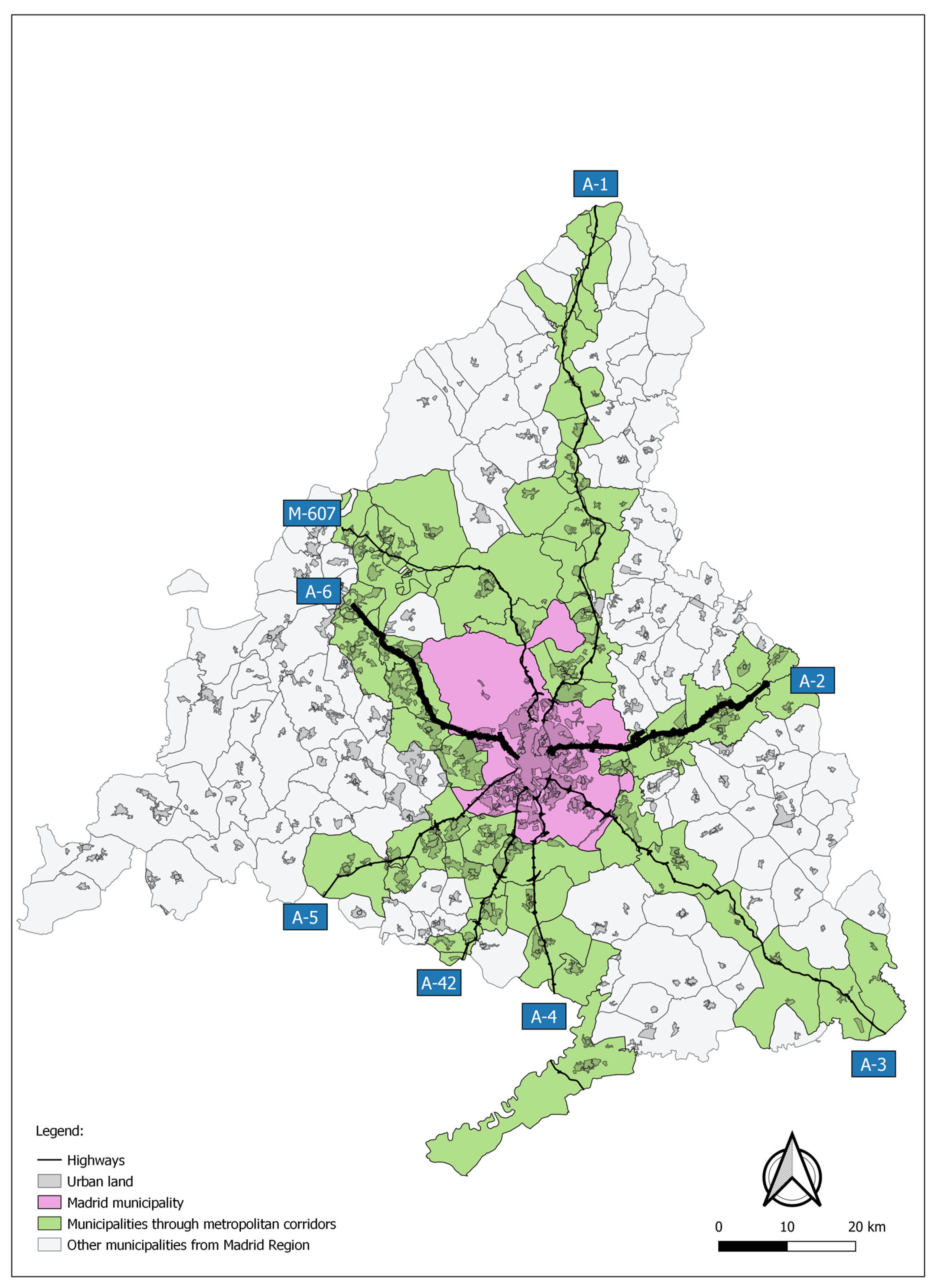
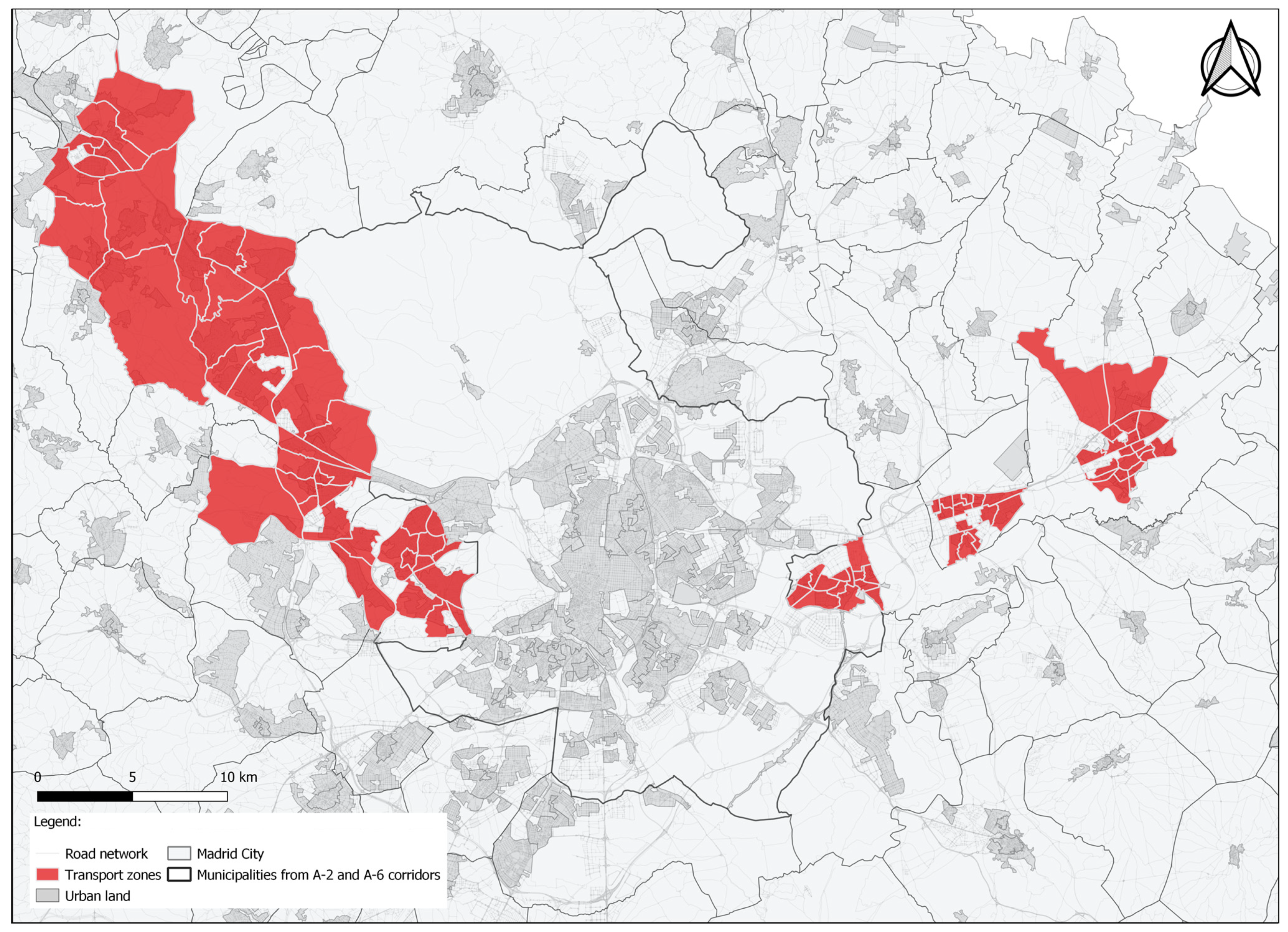
2.1. Case Study: Two Metropolitan Corridors in Madrid

The Madrid Region has a population of 6.5 million inhabitants, distributed in 179 municipalities. The main municipality and core city of the region is Madrid, a central area where 3.2 million people live. The territorial distribution is associated with its major road infrastructures: eight radial motorways connected by three circular rings (Figure 1). These main road infrastructures act as different transport corridors that are the backbone of land use and mobility in all of the region [42].

Table 1. Broad characteristics of the eight transport corridors in Madrid Region (rounded values).

Corridor	Population * (1000 Inhabitants)	Average Gross Income * (1000 € per Inhabitant Per Year)	Daily Traffic * (1000 Cars Per Day)
A-1	250	50	90
A-2 *	600	30	135
A-3	200	30	85
A-4	550	25	125
A-42	750	25	110
A-5	750	30	90
A-6 *	550	55	140
M-607	300	45	80

Data source: INE (2022). * Selected corridors for the study.

shows the broad characteristics of the corridors. The population in the Madrid Region is especially concentrated in the South (i.e., A-42 and A-5). Southern corridors are generally characterized by residential land use and lower household incomes. Northern corridors A-1 and A-6 are important tertiary axes, although A-6 also concentrates a great amount of the population. In the eastern A-2 corridor, we can find important population cores as well as industrial areas. The decision made by the consortium of U-MOVE was to select the A-2 and A-6 corridors as case studies for the project. A variety of reasons support this decision. Firstly, these corridors carry the heaviest traffic flows, being also comparable in population. Secondly, both corridors are different in terms of land use—as mentioned above—and income levels: the A-6 corridor presents the highest average income while income levels in the A-2 corridor correspond to the middle–low class segments. Thirdly, both corridors have good connections with the Madrid City Center, through commuter trains, intercity buses, and metro or light rail. Finally, a comparative analysis between both corridors may be of interest from a strategic point of view. Due to the fact that a Bus–HOV lane was implemented in the A-6 by 2004, and partly because of the success of this initiative, another Bus–HOV lane is planned for the A-2 corridor in the near future.

2.2. Indicators to Characterize Urban Mobility in the Case Study

In this research, indicators are used to explore those urban characteristics determining daily mobility. The explanatory variables to be considered are extracted from a literature review of previous studies with similar objectives (Section 2.2.1). The selection and calculation of indicators to measure these variables are performed according to available information and data sets in the case study (Section 2.2.2).

2.2.1. Literature Review: Concepts and Variables Surrounding Urban Mobility

The term urban mobility is here understood as the total sum of individual trips [43]. Therefore, urban mobility does not only depend on transport systems, but also on the socioeconomic characteristics of individuals, the built environment, and its spatial distribution [9,44,45]. The studies summarized below deepen these relationships. The different variables considered in each study are summarized in

Table 2. Concepts determining urban mobility and related variables (from literature reviewed).

Determinants of Urban Mobility			References (Literature Review)
	Key Concepts	Variables	(a)	(b)	(c)	(d)	(e)	(f)	(g)	(h)	(i)	(j)	(k)	(l)
Socioeconomic and personal characteristics	Demographic distribution	-Children -Elders -Working-age people -Gender				X	X	X			X	X	X
	Socio-economic features	-Household income -Household size -Educational level		X	X		X	X		X	X
Land-use attributes and urban form	Density and diversity	-Inhabitants per hectare -Land use -Activities (e.g., schools, health centers, shops)	X	X	X	X	X		X				X	X
	Accessibility	-Existence of railway station -PT services -Configuration of streets (e.g., no. of intersections)	X	X		X		X		X		X	X	X
	Geographical situation	-Distance to the city center	X								X	X	X
	Urban size and form	-Population in the municipality -Shape index	X			X	X		X	X		X
Urban transport patterns	Car availability and modal choices	-Modal share (car/PT/bike/walking) -Car availability	X		X	X	X	X		X	X	X	X
	Trip characteristics	-Travel distance -Time and timetables -Trip purposes			X	X	X	X		X	X	X	X

, and are the basis for the indicator’s selection:

• (a) Handy [28] carries out a review of different approaches trying to understand the relation between urban form and travel behavior. She remarks on the importance of providing alternatives to using a car through urban design, especially in new developments. Walking is promoted if residential areas are provided with facilities such as shops, schools, or health centers. Public transport may be an option if there is a competitive offer of services. In this regard, it is especially relevant to consider the connections by train;
• (b) Kockelman [29] also focuses on the influence of variables related to urban form on residential mobility. She analyzes the case of the San Francisco Bay Area, finding that a balanced land use mix and accessibility levels could be more relevant than other variables usually used to predict travel behavior. Nevertheless, demographic and socioeconomic variables should never be neglected;
• (c) Giuliano and Narayan [30] explore the relationship between land-use characteristics and individual mobility. They make a comparison between the US and Great Britain using travel diary data. According to this research, differences in daily trips and miles traveled are mainly explained by household income and urban density;
• (d) Zang [31] uses data from a travel survey in Boston to analyze how spatial accessibility may explain non-work travel choices. Apart from accessibility, many other explanatory variables are included in this research (see Table 2). Special importance is attached to household characteristics such as size, composition, and proximity to facilities such as schools or leisure areas;
• (e) Giuliano and Dargay [32] extend the study carried out in [c]. Results show that apart from income and density, other variables related to demography, population size, or car ownership and costs are also explanatory factors for urban mobility;
• (f) The analysis presented by Limtanakool et al. [33] shows how socioeconomic factors, land use characteristics, and travel time affect mode choice. The authors employ data from the 1998 Netherlands National Travel Survey in the analysis, and also emphasize the importance of trip purposes when choosing the transport mode;
• (g) Kang et al. [34] investigate how mobility patterns are affected by compactness and urban size. This research is quite different from previous ones. On the one hand, the authors only consider two variables, carrying out a very thorough analysis of both. On the other hand, mobility phone data instead of household survey data are used to characterize travel patterns. The study includes eight cities in Northeast China;
• (h) Klinger and Lanzendorf [35] apply regression models to analyze the determinants of modal choices in the context of three German cities. They focus on the variables related to urban form, socioeconomics, and transport infrastructure and offer. Data are extracted from a survey specifically conducted for the research;
• (i) Bel and Rosell [36] use a household travel survey to analyze the factors influencing the greenhouse gas emissions of individuals on their daily trips. The variables analyzed are mainly related to personal characteristics (e.g., occupation, age, gender, educational level, or income). The case study is the metropolitan area of Barcelona, and the mapped results show the importance of the geographical situation in relation to the city center;
• (j) Marcinczak and Bartosiewicz [37] determine the relations between commuting patterns and urban form in Poland. This study focuses on the effect of spatial structure on daily trips made for work. Conclusions are critical with the trends towards suburbanization, but the analysis only considers jobs’ locations;
• (k) Reul et al. [38] quantify the effects of potential influencing factors on urban transportation in the future through an innovative approach. The results are based on an activity-based transport demand model, developed for a synthetic city. The authors analyze different scenarios to investigate urban transportation against the backdrop of mode availability, urban structure, or an aging population;
• (l) Cerin et al. [39] focus on a cross-cutting topic, which is becoming increasingly significant: synergies between transport and health. They analyze how local urban design features may encourage walking. To that end, data from specific surveys carried out in 14 cities around the world are combined with objective measures of the built environment. The results, presented at the neighborhood level, show that the main factors predicting walking share are: the density, the number of intersections and the public transport connectivity.

These 10 studies reviewed constitute an appropriate framework to conceptualize and define the main variables surrounding urban mobility (Table 2). Most of them gather data from mobility surveys to analyze transport patterns as dependent variables of other variables, as is the case for this research. However, there are clear differences in at least three aspects—the variables, the contexts, and the type of trips analyzed:

• Concerning the variables, some of them are more focused on urban form or land use attributes (e.g., (a) [28], (g) [34], and (l) [39]). Others are more focused on socioeconomic and personal characteristics (e.g., (i) [36]). Additionally, there are more broad studies trying to include a range of socioeconomic and land use variables (e.g., (d) [31] and (e) [32]).
• As for the formal contexts, there is a wide variation. There are approaches that analyze only one city or metropolitan area (e.g., (b) [29], (d) [31], and (i) [36]), while others include in their analysis various cities or adopt a national or even international approach (e.g., (c) [30], (e) [32], (f) [33], (h) [35], and (j) [37]). In reference to the case studies, the most innovative approach is based on the analysis of a synthetic city through an activity-based transport model (k) [38].
• Finally, although most studies consider all types of daily trips, we also find investigations only addressing commuting trips (e.g., (j) [37]) or non-work travel (e.g., (d) [31]).

As regards to the first aspect, the variables, this research intends to adopt a more comprehensive approach than previous studies. Thanks to the extensive literature review, all key concepts and associated variables that could explain urban mobility are considered, unless there are data restrictions. In respect of the second aspect, the context of analysis, the study presented here analyses the transport zones in two metropolitan corridors of the Madrid Region. This perspective is particularly novel. Despite the relevance of suburban trips—commonly characterized by car dependence—research specifically addressing suburban mobility and its determinants is scarce [15,16,17,25]. Finally, we address all types of trips and purposes on an aggregated basis. In the Madrid Region, 57% of trips respond to occupational mobility and 43% to non-occupational mobility [46]. Therefore, any partial analysis only considering either commuting trips or non-work travel would be leaving aside an important part of everyday mobility.

2.2.2. Data Availability and Indicators

This research aims to understand the main factors shaping urban mobility. Because mobility is the result of individual trips, from now on we will consider the variables related to transport patterns as dependent variables (e.g., modal share indicators). Through different methodologies, we explore the interactions between transport variables and other independent variables listed above (Table 2) related to socioeconomic characteristics or urban configuration. Therefore, data collection depends on the configuration and zonification of transport indicators. In this regard, the most valuable data source to gather data concerning residential transport behavior are Household Mobility Surveys (HMS) [47]. In the Madrid Region, an HMS was carried out in 2018 [47], which has been the main data source for this study. The sample of this survey, based on personal interviews, consists of 85,064 people, distributed into 1259 transport zones [46]. These transport zones were delimited to try to obtain uniform areas in terms of socioeconomic and urban characteristics, and are the basis for the collection and aggregation of all the indicators. Figure 2 shows the transport zones affected by the two metropolitan corridors analyzed in this research (n = 91), which divide the municipalities into smaller areas.

The data sources where the information about the variables in Table 2 may be available are described below (named by capital letters in alphabetical order A–K). These data sets determine the selection of indicators and related variables:

• (A) Household Mobility Survey (HMS) for the Madrid Region [48]. This is the most important source of information that has served to structure and organize by zones all the data gathered. It provides transport variables such as modal share;
• (B) Open Data from Madrid Transport Authority [49]. This database contains information regarding Public Transport (PT) offer and infrastructure. The data are provided in Geographical Information Systems format. The information is provided for each PT stop and line; therefore, the data must be aggregated to obtain the indicators per transport zone;
• (C) Geographic Information from the Spanish Ministry of Transport and Urban Agenda [50]. The information available here is very wide and diverse and covers the national territory. Of special interest in this case is the information on soil classification, urbanized surface, and population. Data are presented as homogeneous areas considering their land use characteristics. Therefore, some transformations—generally aggregations—are needed to obtain the indicators for different territorial divisions;
• (D) Territorial Information System from the Statistic Institute in Madrid Region [51]. It includes cartography and a street map with detailed information for each street. This data source is very useful to calculate distances, or to obtain information on activities and the supply of services existing in different zones of the Region. However, it is necessary to simplify the figures to calculate the indicators per transport zone. For example, the number of activities is provided per street and must be aggregated. While the estimation of distances to the city center is based on the centroids of the zones;
• (E) Spanish Statistical Institute [52]. Statistics on population, demography, and socioeconomic characteristics of residents per zone can be found in this data source. Some figures in this source are obtained at the municipal level, and therefore certain disaggregation is needed to obtain the indicators.

Table 3. Indicators and databases.

Variables from Literature Review	Selected * and Calculated Indicators Per Transport Zone (Units)	Reference Year and Comments	Databases (X) Data Available (✓) Data Used
			[A]	[B]	[C]	[D]	[E]
-Children -Elders -Working-age people -Gender	-Population under 14 (%) -Population over 65 (%) -Working age population (%) -Women (%)	Year 2018. Data on [E] are more complete and solid as it comes from electoral roll and not from a statistical sample	X				✓
-Household income -Household size -Educational level	-Net household income (€/year)	Year 2018	X				✓
-Inhabitants per hectare -Land use -Activities (e.g., schools, health centers, shops)	-Urban density (Inhabitants/ha)	Year 2021. This indicator requires information on soil classification (urban areas), available in [C], and population, available in [E]. Information on these sources is provided up to date (reference year 2021)			✓		✓
	-Aggregated activities (No./ha)	Year 2021. Information on aggregated activities (i.e., schools, health centers, and commerce) is available in [D] and provided up to date (reference year 2021)				✓
-Existence of railway station -PT services	-Population near a train station <800 m (%) -PT stops (No./ha)	Year 2021. Data for public transport offer are available in [B] and values of population and buffers are provided by [C]		✓		✓
-Distance to the city center	-Distance to the city center (km)	Year 2021. Average distances to the city center are calculated through [D]				✓
-Population in the municipality -Shape index	-	Since transport zones are smaller than municipalities (Figure 2), these indicators are not appropriate to the context			X		X
- Modal share (Car/PT/ Bike/Walking) -Car availability	-Car share (%) -PT share (%) -Walking share (%) -Car availability (no. vehicles per Inhabitant)	Year 2018	✓
-Travel distance -Time and timetables -Trip purposes	-Average travel distance (km)	Year 2018. Information on time and timetables or trip purposes is also available in [A], but data are provided in categorical formats, not easily transformed into numerical variables (therefore discarded)	✓

* Selection criteria: available information, transparent indicators which are easy to understand. Variables easily presented into numeric formats.

shows the indicators finally calculated in this research and specifies the databases used for collecting the necessary information. The indicators have been calculated by compiling the available data per transport zone. The selection and calculation of indicators follow the conceptual framework and taxonomy extracted from the literature review (Table 2). Additionally, the indicators finally used meet the requirements specified by [53], being transparent and easy to understand and measure. This criterion means that indicators such as household size are discarded in favor of others such as income, which is easier to understand and measure. Finally, as the methodologies in this research include correlational and cluster analyses, indicators should be easily transformed into numerical variables.

2.3. Correlation Analysis for Explaining Urban Mobility

One of the objectives of this research is to examine how different urban variables shape urban transport patterns. Two types of correlation tests are employed for this: the Pearson correlation coefficient and Spearman rho. Indicators related to the modal share and car availability are considered dependent variables, which could be explained through variables related to demography, socioeconomic features, density and diversity, PT accessibility, and geographical access (Table 2, 2nd column).

The Pearson correlation analysis is applied by Haghshenas and Vaciri [54] and later by Alonso et al. [4] for similar purposes. Both studies analyze various cities from an aggregated perspective and correlate the variables of city size, density, and GDP with private and PT modal share (samples: n = 100 and n = 23 cities respectively). The research presented in this paper is much more detailed and disaggregated. Indicators are analyzed per transport zone and not per city (sample: n = 91 transport zones), and the range of concepts considered is broader and carefully selected thanks to the literature review carried out (Section 2.2.2). However, for the analysis to be valid, at least one of the variables must be normally distributed [55,56]. A very widespread method to check if variables are normally distributed is the Kolmogorov–Smirnov and Shapiro–Wilk tests. If the test is not significant (Sig. > 0.05 for 95% confidence level), it means that the distribution of the sample is probably normal [56].

Table 4. Normality test results (of indicators proposed in Table 2).

	Kolmogorov–Smirnov			Shapiro–Wilk
	Statistic	df	Sig. (>0.05)	Statistic	df	Sig. (>0.05)
Car share (%)	0.120	91	0.002	0.954	91	0.003
PT share (%) *	0.084	91	0.122	0.980	91	0.183
Walking share (%)	0.108	91	0.010	0.950	91	0.002
Car Availability (no. vehicles per inhabitant) *	0.065	91	0.200	0.987	91	0.533
Average travel distance (km)	0.269	91	0.000	0.426	91	0.000

(*) Normal distribution.

shows the results of this test for the transport variables (dependent variables).

From Table 4 we can observe that only PT share and car availability indicators are normally distributed. Therefore, correlations of these three variables with others are analyzed through the Pearson coefficient (1):

$$\mathrm{Pearson}\mathrm{Correlation}\mathrm{Coefficient}=\frac{\sum \left(x_i-\overline{x}\right)\left(y_i-\overline{y}\right)}{\sqrt{{\left(x_i-x\right)}^2{\left(y_i-y\right)}^2}}$$

(1)

• x_i = values of the x-variable in a sample.
• $\overline{x}$ = mean of the values of the x-variable.
• y_i = values of the y-variable in a sample.
• $\overline{y}$ = mean of the values of the y-variable.

The value of the Pearson correlation coefficient falls in the interval −1 and 1. Being closer to −1 represents a strong negative correlation and being closer to 1 represents a strong positive correlation [57]. Coefficient values of ±0.1 are generally considered to represent a small effect, ±0.3 a medium effect, and ±0.5 a strong effect [56].

The three non-normal dependent variables (i.e., car share, walking share, and average travel distance) are analyzed through Spearman rho. This Spearman correlation coefficient is a non-parametric statistic and so can be used when the data have violated parametric assumptions (e.g., for non-normally distributed data) [58]. It works by first ranking the data and then applying the Pearson equation, and therefore interpretations are similar for both coefficients regarding their values, ranges, and signs. The significance analysis depends on the sample size; the smaller the sample, the higher the Pearson or Spearman coefficients will have to be to prove the correlation between variables. According to agreed formulations linking significance and sample size in the Pearson and Spearman methods, a sample of 28 is enough to detect strong correlations, and samples bigger than 84 are needed to confirm small effects between variables [59]. In this case, the sample (n = 91) is large enough to capture all strong and medium effects and even some small effects.

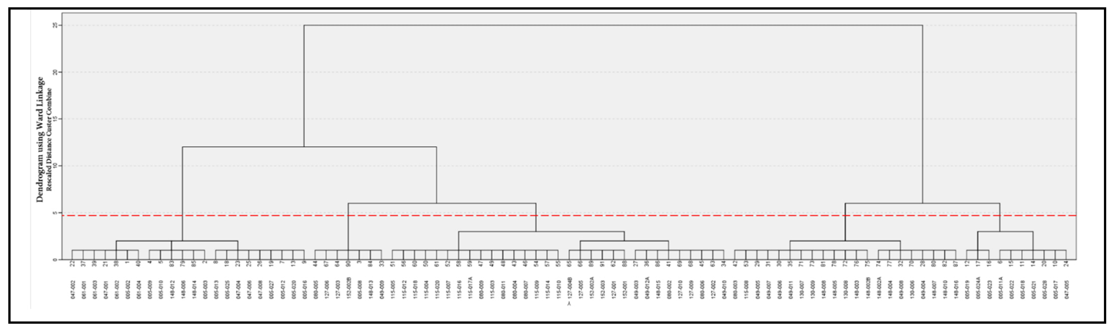
2.4. Cluster Analysis to Classify Transport Zones According to Mobility Patterns

The study of the A-2 and A-6 metropolitan corridors through indicators compiled by transport zone implies considering data from 91 zones. This gives a picture not easily interpretable. The picture could be simplified if the information was analyzed on an aggregated basis (e.g., by corridor or for the two corridors), but then many specificities would be lost. Urban and suburban zones in the metropolitan regions may be totally different from one another, even if they are geographically close [36]. As an intermediate solution to simplify this outlook, the 91 zones are classified into homogeneous groups according to their socioeconomic and urban form characteristics. This allows the analysis of the transport patterns characteristic of each type of zone without losing important specificities, but at the same time makes the presentation and interpretation of data easier.

The method used for the classification is the cluster analysis, which aims to reduce the dimensionality of a data set by exploiting the similarities and dissimilarities between the cases (the transport zones) [4]. The approach is hierarchical if the classification has an increasing number of nested classes, and non-hierarchical if the number of clusters is previously decided [60].

The first and most important step of the cluster analysis is the selection of appropriate variables considering the objective of the classification [61]. Hair et al. [62] set out two main recommendations to select the variables. Firstly, variables should relate specifically to the objectives of the cluster analysis. In this case, the objective is to create a taxonomy able to provide a clear image of the types of zones existing in the metropolitan corridors, in terms of geographical location and urban and social conditions. Therefore, indicators related to all these key concepts (defined in Table 2) should be included in the classification. Secondly, it is not appropriate to include too many variables. Instead, it is better to include one variable for each concept and ensure that they are relevant to the main objective. In response to the primary objective of this research, the taxonomy should also explain the different mobility patterns existing in the different types of zones. For these reasons, just one indicator per key concept is selected. Where there is more than one indicator available per key concept, their impact on transport patterns is considered (i.e., higher impacts are preferred, according to the correlation coefficients). This criterion also avoids substantial multicollinearity among selected indicators as classification variables. The existence of multicollinearity does not invalidate the statistical results of the cluster analysis, but it is not desirable as it may indicate that some concepts are being double-counted.

The procedure followed for the cluster analysis in this research is the one proposed by Alonso et al. [4], composed of several stages and supported by a strong theoretical basis [61,62]. The objectives of both studies are similar: classifying cities to analyze the sustainability of their transport systems in Alonso et al. [4], and classifying transport zones to understand the factors shaping mobility patterns in this case. The sample in this research is larger (n = 91 transport zones) compared to the sample of 23 cities analyzed in the reference study. This difference may be positive to obtain significant groups and results [62]. The stages of the procedure are summarized below:

• Normalize selected indicators using Z-scores formulation;
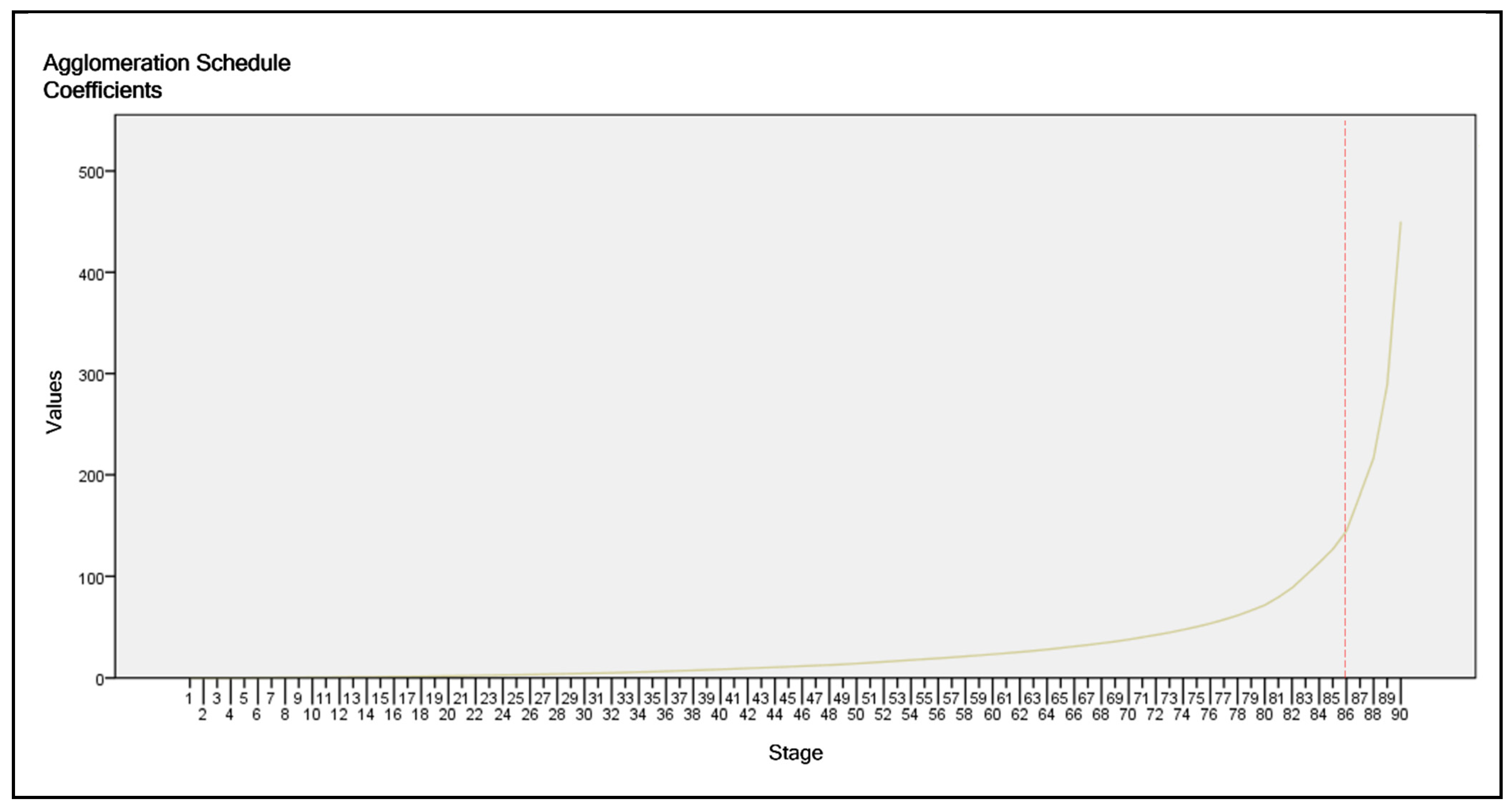
• Set the appropriate number of clusters through a hierarchical method: the Ward method with squared Euclidean distance measurement. The number of clusters is set according to the agglomeration schedule and the dendrogram;
• Use the non-hierarchical method k-means to test the stability of the resulting clusters. The number of clusters is defined in stage 2 and the iterations are started from centroids obtained with the Ward method;
• Test the validity of the obtained solution. On the one hand, by comparing the solutions obtained by the two cluster methods used; on the other hand, through the ANOVA analysis, which shows if the classification variables selected contribute to the cluster classification.

3. Results

In this section, the results of the correlation and cluster analyses of the zones are presented. The use of the Household Mobility Survey [48] as the main database involves certain limitations. Some zones are excluded from the analysis because the sample of surveys carried out in the zone is not enough to consider the information representative. This is the case of 44 zones out of the 135 comprised in the A-2 and A-6 corridors. Therefore, analyses are performed for 91 transport zones. The zones excluded are mostly located in the A-2 corridor, corresponding to industrial areas where very few residents live. We may also find some areas excluded in the A-6 corridor, mainly characterized by tertiary activities. Therefore, it is assumed that the final sample is representative of the residential areas in both the A-2 and A-6 corridors.

3.1. Explanatory Variables for Urban Mobility Patterns

Results from the Pearson and Spearman tests are shown in

Table 5. Correlation coefficients between transport variables and explanatory variables.

		Transport Variables
		Normal Variables		Non-Normal Variables
Key Concepts	Explanatory Variables	PT Share	Car Availability	Car Share	Walking Share	Average Travel Distance
Demographic distribution	Population under 14 (%)	−0.080	0.378 **	0.659 **	−0.633 **	0.439 **
	Population over 65 (%)	0.166	−0.348 **	−0.553 **	0.484 **	−0.333 **
	Working age population (%)	−0.183	0.135	0.188	−0.126	0.130
	Women (%)	0.064	0.011	−0.059	0.029	0.105
Socio-economic features	Net household income (€/year)	0.354 **	0.523 **	0.705 **	−0.737 **	0.495 **
Density and diversity	Urban density (Inhabitants/ha)	−0.069	−0.613 **	−0.812 **	0.799 **	−0.582 **
	Aggregated activities (No./ha)	−0.059	−0.487 **	−0.735 **	0.702 **	−0.533 **
Accessibility	Population near a train station <800 m (%)	0.244 *	−0.078	−0.160	0.080	0.002
	PT stops (No./ha)	0.009	−0.517 **	−0.753 **	0.715 **	−0.506 **
Geographical situation	Distance to the city center (km)	−0.384 **	−0.296 **	−0.174	0.269 **	0.205
		(Pearson coefficient)		(Spearman rho)

** Correlation is significant at level 0.01 (2-tailed). * Correlation is significant at level 0.05 (2-tailed).

in the form of correlation coefficients. Significant coefficients imply causality between variables: at the 95% confidence level if marked with two asterisks (**), or 90% confidence level if marked with one asterisk (*). Furthermore, it is considered that absolute values higher than 0.5 indicate strong effects [56]. Therefore, we can infer the following relationships between transport variables and other explanatory variables:

• Regarding the demographic distribution, the existence of children and elders are both relevant variables shaping mobility in contrary directions. In those zones with a higher percentage of the population over 65, the transport patterns are more sustainable. The use and availability of cars are substantially lower, the walking share is higher, and the trips are shorter. The rate of children has a stronger and opposite effect, especially on the car share and walking share. Those zones with a higher percentage of the population under 14 are very car-dependent and are characterized by few walking trips. As for the working-age population or women rates, no significant relations can be demonstrated with transport variables, at least at the zone level.
• Concerning the socioeconomic concept, results attach great importance to income levels as explanatory variables. In this suburban context, wealthier families live in zones where the car share is particularly higher, while the walking share is particularly lower (absolute coefficient values > 0.7). These high-income zones are also characterized by car availability and long distances traveled. The positive correlation between income and the public transport share may be surprising. This is because the wealthiest zones are located not very far from the city center and have good quality radial connections by public transport (e.g., many zones in the A-6 corridor are connected with Madrid City by a Bus–HOV lane).
• Density and diversity play the most important role in shaping mobility. The number of inhabitants per urban surface is the variable with the biggest influence on transport variables. Correlation coefficients demonstrate that in low-density settlements, the motorization rate and especially the use of cars is higher. By contrast, people living in more compact urban areas make shorter trips and walk more. As for diversity, those areas with a broader offer of activities and services show more sustainable travel patterns: less dependence on cars, more trips on foot, and shorter distances. The public transport share is the only transport variable that is not well explained by any of these density or diversity-related variables.
• Regarding the accessibility to public transport, those urban areas close to a train station (800 m buffer) present higher PT use. However, the effect is moderate. As for the number of PT stops, it has a very high effect on car share but the effect on PT use is not significant. In this metropolitan context, the public transport share is found to be an indicator with little variation (ranging from 10 to 20%) compared to the car (from 30 to 70%) or walking shares (from 20 to 60%). This makes it difficult to find strong correlations with the rest of the variables.
• Finally, the distance to the city—the center of the Madrid Municipality—is a very interesting explanatory factor. It is the variable with the highest impact on the public transport share, even if the effect is not very strong (Pearson coefficient < 0.5). As would be expected, people living closer to the city center make more trips by public transport. However, living far from the city center does not necessarily imply having less sustainable transport patterns. In fact, distant zones present higher walking shares and lower motorization rates. Precisely due to the distance, many of these zones work as isolated areas, being self-sufficient for many functions.

3.2. Transport Zones Classification

According to the criteria established in Section 2.3, the variables selected for the classification (one per key concept, prioritizing those with the highest impact on mobility patterns) were population under 14, net household income, urban density, no. PT stops, and distance to the city center. Then, following the steps also described in the methodological section, five clusters were identified as the optimal solution (See Appendix A). The five clusters are described in

Table 6. Average profile of transport zones in each cluster (See Figure A1).

Indicators	Cluster 1 (n = 10)	Cluster 2 (n = 24)	Cluster 3 (n = 21)	Cluster 4 (n = 9)	Cluster 5 (n = 27)
	Self-Sufficient Dense Zones, with Aging Population and Far from City Center	Middle-Class Dense Zones in the East, Closer to City Center	Middle-Class Zones with Low Density and Far from City Center	Upper-Class Families with Children and Very Car-Dependent	Wealthiest Zones with Very Low Density and Few Local Activities
Population under 14 (%)	12	13	16	24	16
Population over 65 (%)	22	19	14	8	17
Working age population (%)	65	68	70	67	67
Women (%)	52	51	51	51	52
Net household income (€/year)	32,081	37,265	41,964	60,054	77,664
Urban density (Inhab./ha)	268	175	55	39	34
Aggregated activities (no./ha)	13.8	11.4	6.2	4.3	3.4
Population near a train station <800 m (%)	39.1	21.7	17.6	27.8	15.4
PT stops (no./ha)	75	39	18	12	16
Distance to the city center (km)	30.1	16.4	30.4	19.9	14.7
Car share (%)	28	37	51	67	62
PT share (%)	14	14	13	12	18
Walking share (%)	57	48	35	20	18
Car availability (no. vehicles per inhabitant)	0.54	0.64	0.68	0.74	0.73
Average travel distance (km)	7	4	6	11	6

, and graphically represented in Figure 3:

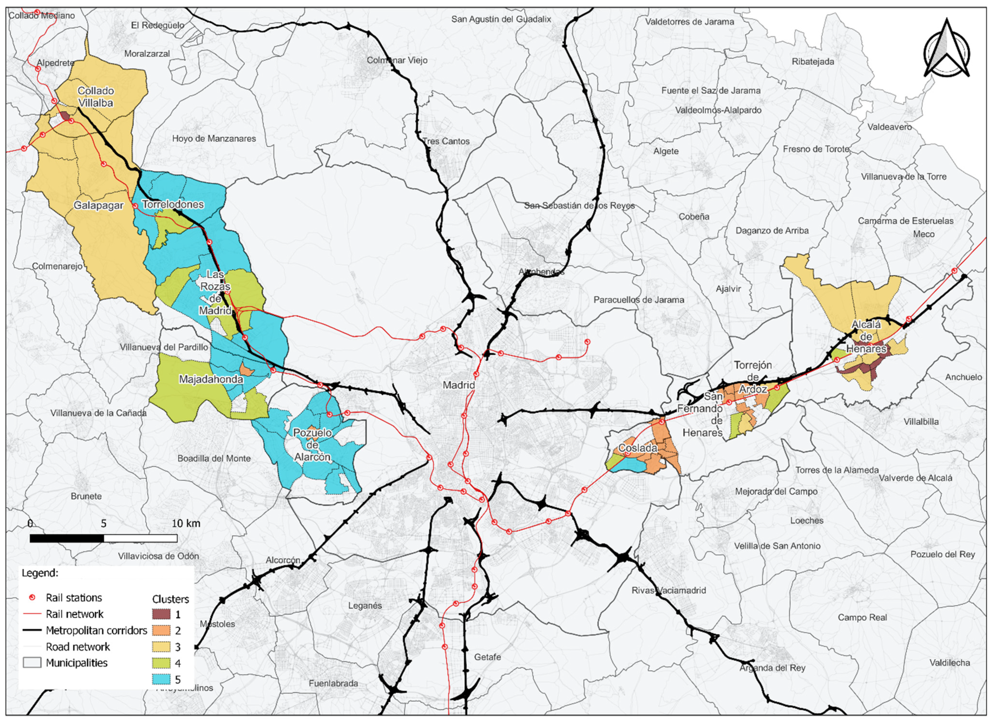
• Cluster 1: Self-sufficient dense zones, with an aging population and far from the city center. This cluster is composed of the zones with the highest urban density (268 Inhab./ha). Most of them are historical centers, with few children (12% on average) and many elders (22%). These zones are functional urban centers far away from Madrid city (30 km) and well provided for by services and activities, which are viable thanks to the urban density. They present the highest walking shares (57% of the trips on foot) and the lowest use of cars.
• Cluster 2: Middle-class dense zones in the East, closer to the city center. These zones are also very dense and well provided for. They are in the A-2 corridor, relatively close to the Madrid city center (16 km on average). The income is higher than zones in Cluster 1 but low compared to other zones in this sample, especially those located in the A-6 corridor. Nearly half of the trips are made on foot. Due to their high walking shares and their proximity to Madrid, people living in those zones make the shortest trips in this sample (4 km).
• Cluster 3: Middle-class zones with low density and far from the city center. The zones in this cluster are very far from Madrid city (30 km). Despite the distance, they do not work as self-sufficient centers due to their lack of activities and services and their lower density compared to equally distant zones in Cluster 1 (55 Inhab./ha). More than half of their trips are made by car.
• Cluster 4: Zones with upper-class families with children that are very car-dependent. Zones characterized by a young population, showing the highest percentage of children (24%). Families living in these areas are wealthy and very car-dependent (0.74 cars per inhabitant and 67% of trips by car). Few activities are offered in these areas and residents have the longest trips (11 km on average).
• Cluster 5: Wealthiest zones with very low density and few local activities. This cluster is composed of the most dispersed zones (34 Inhab./ha). Households with the highest incomes live in these zones (77,664 € per year), which are located mainly in the A-6 corridor. Most trips are made by car (67%), and very few on foot. As for public transport use, it is high compared to the rest of the clusters (18% of the trips). This is probably due to the proximity to Madrid city and the relatively good connections by PT with the city center.

4. Discussion

One of the main objectives of this research is to determine the key concepts and variables explaining mobility patterns in suburban areas. As in other studies, a statistical correlational analysis is carried out to describe these interactions. The main findings of this analysis are described in the following paragraphs and compared with results from previous research.

Regarding demography, two variables have strong and opposite effects on car share and walking share: the rates of the population under 14 and over 65. Zones with higher percentages of children are more car-dependent, while walking trips are more recurrent in zones with many people aged over 65. These results are foreseeable and consistent with previous research (e.g., [32,36]). However, the approach here is clearer and more detailed and the results are more categorical (higher correlations are found). Giuliano and Dargay [32] just consider the percentage of elders while Bel and Rosell [36] consider the average age of the population. As for the variable gender, in contrast to other studies [36], it does not explain differences in transport patterns between different zones. This is due to the approach of the study. At the individual level, differences in mobility patterns between men and women have long been demonstrated [63]. However, if indicators are examined at the transport zone level, the percentage of each sex is close to 50%, with small variations towards a majority of women due to their higher average life expectancy. These little variations make it impossible to establish causal relations with any transport variable. A more detailed study, with different data segmentations, would be needed to explore gender differences in transport patterns.

Income levels are positively correlated with the use of cars and negatively correlated with active modes. This causality is also found in previous studies [35,36]. However, these results would probably be very different if the context of analysis was the municipality of Madrid and not its metropolitan surrounding area. As Carpio-Pinedo et al. [64] demonstrated, in the Madrid city center higher incomes are usually located in areas well provided for by services, commerce, and activities.

The study reveals that variables related to density and diversity are the most powerful to infer car dependence and active mobility. In this regard, denser areas with mixed land use present more sustainable transport patterns. This statement is commonly agreed to in the literature, and the results just ratify the findings of previous studies (e.g., [28,30,31,34]). However, neither the density nor the mix of activities predict public transport patronage. This is a surprising outcome that contradicts conclusions obtained in other studies (e.g., [4,30,32]), and it is probably due to the context of this research. Previous studies analyze information on an aggregated basis, mixing data from zones in the city center with data from suburban zones. Results in these simplifications are statistically very influenced by the performance of central areas, with high density and high public transport patronage. While in the metropolitan context, this interdependence is not so clear.

Nevertheless, it is noted that public transport share is not very well explained by the variables included in this study. It seems that areas with a higher income, closer to the city center, and connected by railway tend to use more public transport. However, according to the correlation coefficients obtained, these effects are not very strong. A deeper analysis would be needed to explain public transport use. On the one hand, more complex accessibility measures based on the quality of services (i.e., including quantity and frequency of services and not only the number of stops) would probably be better predictors [65,66]. On the other hand, analysis considering travel purposes and timetables could help to understand the reasons behind public transport modal choice [31,37]).

The effects of geographical distance to the city center over certain transport variables might be, a priori, surprising. It seems that people living further from the Madrid city center tend to walk more. This refutes findings from other studies (e.g., [36]). It is because there are some zones in the outer periphery working as self-sufficient urban centers. These zones are also characterized by higher densities, a broad offer of services and activities, and lower motorization rates (e.g., zones in Cluster 1).

In addition to the correlational tests, an exploratory analysis is carried out: the cluster analysis. None of the studies reviewed applied exploratory statistics or cluster analysis for a similar approach, and in this case, the results are clarifying. Specifically, it shows significant differences between the five types of zones (clusters) identified. These differences should be carefully considered, because they may lead to misinterpretations when processing aggregated data, as is the case of most studies on this topic (e.g., [4,30,33,34,35,37]).

5. Conclusions

Initiatives addressing daily mobility pay little attention to the suburbs, at both policy and scientific levels. However, the population is precisely growing in the peripheries of core cities, where transport patterns are generally less sustainable. This study aims to understand the factors determining mobility patterns in the context of two metropolitan corridors in the Madrid Region. Its originality is firstly based on the specificity of the context, the suburban areas; secondly, on its broad approach. Thanks to the exhaustive literature review, all the key concepts and related variables surrounding mobility are considered, except for some data limitations. Finally, the twofold methodology is novel and useful to describe the complex interrelations between urban characteristics and mobility patterns and the taxonomy of zones existing in peripheries.

Regarding the conceptual outcomes of the research, the first one is a list of key concepts and related characteristics (variables) that, according to the literature, may shape daily mobility (Table 2). This can be a useful input for future research. We find that the most recurrent concepts in previous studies are socioeconomic features, density and diversity, accessibility, and urban size and form.

Secondly, the interrelations between certain variables and transport patterns are examined. The main characteristics leading towards higher car use are, by order of importance, low urban density, few local activities, a high percentage of children, and a low percentage of seniors. Apart from these commonly agreed findings, certain results obtained in the correlation analysis are less foreseeable. On the one hand, the distance to the Madrid city center does not explain car use. Moreover, distant zones present more walking trips. This is well understood in the cluster analysis: there are zones far away from the city center but dense and well provided for, that work by themselves as urban centers. On the other hand, public transport use is an indicator with little variation between zones (12–18%) and is difficult to explain through other variables. It seems that wealthier zones closer to the city center tend to use more public transport (due to their privileged connections). However, apart from this, neither density nor accessibility indicators have an effect on public transport use. This is a surprising result, partly due to the suburban context. However, more precise accessibility measures and the consideration of other variables such as travel purposes would be needed to deepen the study into the reasons behind PT use in the peripheries of cities.

Finally, a taxonomy of the types of zones we may find in the suburbs is presented. The 91 transport zones analyzed in the two metropolitan corridors are classified into five clusters, very different from each other. For example, the car share varies from 28% on average in Cluster 1 to 67% in Cluster 4. These differences are explained by their characteristics: Cluster 1 is composed of self-sufficient compact areas with an aging population, while zones in Cluster 4 are typically inhabited by wealthy families with children living in low-density neighborhoods. The differences in the two corridors—the eastern A-2 corridor characterized by a more industrial character and the northeastern A-6 corridor with many tertiary activities and high-income residents—translate into greater concentrations of certain types of zones. For example, zones in Cluster 4 are typically found in the A-6 corridor, although we may also find some examples of these wealthy zones in the A-2 corridor.

Results demonstrate that mobility in the periphery is not necessarily unsustainable if these areas are compact and self-sufficient. This reinforces the theories underlying polycentrism as a solution to the urban sprawl challenge (e.g., [37]).

This research work comes with two main limitations. On the one hand, the statistical methodologies applied require numerical indicators, and therefore some important categorical variables such as travel purposes or timetables are not considered in the analysis. On the other hand, the accessibility measures adopted do not consider the frequency and quality of services and are not able to explain public transport use. These gaps could be addressed in future research. In addition, it would be interesting to replicate the methodology in central areas of the city to compare the results.

References

- Bettencourt, L.M.A.; Lobo, J.; Helbing, D.; Kühnert, C.; West, G.B. Growth, innovation, scaling, and the pace of life in cities. Proc. Natl. Acad. Sci. USA 2007, 104, 7301–7306. [Google Scholar] [CrossRef] [PubMed] [Green Version]
- Nieuwenhuijsen, M.J. Urban and transport planning, environmental exposures and health-new concepts, methods and tools to improve health in cities. Environ. Health 2016, 15, 161–171. [Google Scholar] [CrossRef] [PubMed] [Green Version]
- Newman, P.; Kenworthy, J. Sustainability and Cities: Overcoming Automobile Dependence; Island Press: Washington, DC, USA, 1999. [Google Scholar]
- Alonso, A.; Monzón, A.; Cascajo, R. Comparative analysis of passenger transport sustainability in European cities. Ecol. Indic. 2015, 48, 578–592. [Google Scholar] [CrossRef] [Green Version]
- Nieuwenhuijsen, M.J. Urban and transport planning pathways to carbon neutral, liveable and healthy cities; A review of the current evidence. Environ. Int. 2020, 140, 105661. [Google Scholar] [CrossRef]
- Goldman, T.; Gorham, R. Sustainable urban transport: Four innovative directions. Technol. Soc. 2006, 28, 261–273. [Google Scholar] [CrossRef]
- Attard, M.; Shiftan, Y. Sustainable Urban Transport, 1st ed.; Emerald Group Publishing Limited: Bingley, UK, 2015. [Google Scholar]
- Gallo, M.; Marinelli, M. Sustainable mobility: A review of possible actions and policies. Sustainability 2020, 12, 7499. [Google Scholar] [CrossRef]
- Banister, D. The sustainable mobility paradigm. Transp. Policy 2008, 15, 73–80. [Google Scholar] [CrossRef]
- European Commission. Green Paper—Towards a New Culture for Urban Mobility; COM (2007) 0551 Final; European Commission: Brussels, Belgium, 2007. [Google Scholar]
- European Commission. Action Plan on Urban Mobility; COM (2009) 490 Final; European Commission: Brussels, Belgium, 2009. [Google Scholar]
- European Commission. Together towards Competitive and Resource-Efficient Urban Mobility; COM (2013) 0913 Final; European Commission: Brussels, Belgium, 2013. [Google Scholar]
- Mozos-Blanco, M.Á.; Pozo-Menéndez, E.; Arce-Ruiz, R.; Baucells-Aletà, N. The way to sustainable mobility. A comparative analysis of sustainable mobility plans in Spain. Transp. Policy 2018, 72, 45–54. [Google Scholar] [CrossRef]
- Kiba-Janiak, M.; Witkowski, J. Sustainable Urban Mobility Plans: How Do They Work? Sustainability 2019, 11, 4605. [Google Scholar] [CrossRef] [Green Version]
- De Falco, S.; Angelidou, M.; Addie, J.P.D. From the “smart city” to the “smart metropolis”? Building resilience in the urban periphery. Eur. Urban Reg. Stud. 2018, 26, 205–223. [Google Scholar] [CrossRef]
- Camagni, R.; Gibelli, M.C.; Rigamonti, P. Urban mobility and urban form: The social and environmental costs of different patterns of urban expansion. Ecol. Econ. 2002, 40, 199–216. [Google Scholar] [CrossRef]
- Bassolas, A.; Barbosa-Filho, H.; Dickinson, B.; Dotiwalla, X.; Eastham, P.; Gallotti, R.; Ghoshal, G.; Gipson, B.; Hazarie, S.A.; Kautz, H.; et al. Hierarchical organization of urban mobility and its connection with city livability. Nat. Commun. 2019, 10, 4817. [Google Scholar] [CrossRef] [Green Version]
- McKenzie, G. Urban mobility in the sharing economy: A spatiotemporal comparison of shared mobility services. Comput. Environ. Urban Syst. 2020, 79, 101418. [Google Scholar] [CrossRef]
- Alonso, A.; Monzón, A.; Cascajo, R. Measuring Negative Synergies of Urban Sprawl and Economic Crisis over Public Transport Efficiency. Int. Reg. Sci. Rev. 2017, 41, 540–576. [Google Scholar] [CrossRef] [Green Version]
- Oskarbski, J.; Birr, K.; Zarski, K.; Coelho, M.; Fernandes, P.; Zbieta Macioszek, E. Bicycle Traffic Model for Sustainable Urban Mobility Planning. Energies 2021, 14, 5970. [Google Scholar] [CrossRef]
- Bratzel, S. Conditions of success in sustainable urban transport policyPolicy change in “relatively successful” European cities. Transp. Rev. 2010, 19, 177–190. [Google Scholar] [CrossRef]
- Puhe, M.; Schippl, J. User Perceptions and Attitudes on Sustainable Urban Transport among Young Adults: Findings from Copenhagen, Budapest and Karlsruhe. J. Environ. Policy Plan. 2014, 16, 337–357. [Google Scholar] [CrossRef]
- Magdolen, M.; von Behren, S.; Burger, L.; Chlond, B. Mobility Styles and Car Ownership—Potentials for a Sustainable Urban Transport. Sustainability 2021, 13, 2968. [Google Scholar] [CrossRef]
- Acheampong, R.A.; Cugurullo, F.; Gueriau, M.; Dusparic, I. Can autonomous vehicles enable sustainable mobility in future cities? Insights and policy challenges from user preferences over different urban transport options. Cities 2021, 112, 103134. [Google Scholar] [CrossRef]
- Geneletti, D.; La Rosa, D.; Spyra, M.; Cortinovis, C. A review of approaches and challenges for sustainable planning in urban peripheries. Landsc. Urban Plan. 2017, 165, 231–243. [Google Scholar] [CrossRef]
- Harig, O.; Burghardt, D.; Hecht, R. A Supervised Approach to Delineate Built-Up Areas for Monitoring and Analysis of Settlements. Int. J. Geo-Inf. 2016, 5, 137. [Google Scholar] [CrossRef] [Green Version]
- Litýnski, P. The Intensity of Urban Sprawl in Poland. Int. J. Geo-Inf. 2021, 10, 95. [Google Scholar] [CrossRef]
- Handy, S. Methodologies for exploring the link between urban form and travel behavior. Transp. Res. Part D Transp. Environ. 1996, 1, 151–165. [Google Scholar] [CrossRef]
- Kockelman, K.M. Travel Behavior as Function of Accessibility, Land Use Mixing, and Land Use Balance: Evidence from San Francisco Bay Area. Transp. Res. Rec. J. Transp. Res. Board 1997, 1607, 116–125. [Google Scholar] [CrossRef]
- Giuliano, G.; Narayan, D. Another Look at Travel Patterns and Urban Form: The US and Great Britain. Urban Stud. 2003, 40, 2295–2312. [Google Scholar] [CrossRef] [Green Version]
- Zhang, M. Exploring the relationship between urban form and nonwork travel through time use analysis. Landsc. Urban Plan. 2005, 73, 244–261. [Google Scholar] [CrossRef]
- Giuliano, G.; Dargay, J. Car ownership, travel and land use: A comparison of the US and Great Britain. Transp. Res. Part A Policy Pract. 2006, 40, 106–124. [Google Scholar] [CrossRef]
- Limtanakool, N.; Dijst, M.; Schwanen, T. The influence of socioeconomic characteristics, land use and travel time considerations on mode choice for medium- and longer-distance trips. J. Transp. Geogr. 2006, 14, 327–341. [Google Scholar] [CrossRef]
- Kang, C.; Ma, X.; Tong, D.; Liu, Y. Intra-urban human mobility patterns: An urban morphology perspective. Phys. A Stat. Mech. Its Appl. 2012, 391, 1702–1717. [Google Scholar] [CrossRef]
- Klinger, T.; Lanzendorf, M. Moving between mobility cultures: What affects the travel behavior of new residents? Transportation 2016, 43, 243–271. [Google Scholar] [CrossRef]
- Bel, G.; Rosell, J. The impact of socioeconomic characteristics on CO2 emissions associated with urban mobility: Inequality across individuals. Energy Econ. 2017, 64, 251–261. [Google Scholar] [CrossRef]
- Marcińczak, S.; Bartosiewicz, B. Commuting patterns and urban form: Evidence from Poland. J. Transp. Geogr. 2018, 70, 31–39. [Google Scholar] [CrossRef]
- Reul, J.; Grube, T.; Stolten, D. Urban transportation at an inflection point: An analysis of potential influencing factors. Transp. Res. Part D Transp. Environ. 2021, 92, 102733. [Google Scholar] [CrossRef]
- Cerin, E.; Sallis, J.F.; Salvo, D.; Hinckson, E.; Conway, T.L.; Owen, N.; van Dyck, D.; Lowe, M.; Higgs, C.; Moudon, A.V.; et al. Determining thresholds for spatial urban design and transport features that support walking to create healthy and sustainable cities: Findings from the IPEN Adult study. Lancet Glob. Health 2022, 10, e895–e906. [Google Scholar] [CrossRef]
- Jiménez-Espada, M.; Naranjo, J.M.V.; García, F.M.M. Identification of Mobility Patterns in Rural Areas of Low Demographic Density through Stated Preference Surveys. Appl. Sci. 2022, 12, 10034. [Google Scholar] [CrossRef]
- U-MOVE. Smart Strategies for Urban Sustainable Mobility. Available online: http://umove.transyt-projects.es/ (accessed on 18 October 2022).
- Romero, C.; Monzón, A.; Alonso, A.; Julio, R. Potential demand for bus commuting trips in metropolitan corridors through the use of real-time information tools. Int. J. Sustain. Transp. 2021, 16, 314–325. [Google Scholar] [CrossRef]
- Schafer, A.; Victor, D.G. The future mobility of the world population. Transp. Res. Part A Policy Pract. 2000, 34, 171–205. [Google Scholar] [CrossRef]
- Tyrinopoulos, Y.; Antoniou, C. Factors affecting modal choice in urban mobility. Eur. Transp. Res. Rev. 2013, 5, 27–39. [Google Scholar] [CrossRef] [Green Version]
- Cavoli, C. Accelerating sustainable mobility and land-use transitions in rapidly growing cities: Identifying common patterns and enabling factors. J. Transp. Geogr. 2021, 94, 103093. [Google Scholar] [CrossRef]
- Deloitte; IPD. Encuesta de Movilidad de la Comunidad de Madrid 2018; Consorcio Regional de Transportes de Madrid: Madrid, Spain, 2018. [Google Scholar]
- Nicolas, J.P.; Pochet, P.; Poimboeuf, H. Towards sustainable mobility indicators: Application to the Lyons conurbation. Transp. Policy 2003, 10, 197–208. [Google Scholar] [CrossRef]
- Consorcio de Transportes de Madrid. Available online: https://www.crtm.es/conocenos/planificacion-estudios-y-proyectos/encuesta-domiciliaria/edm2018.aspx (accessed on 18 October 2022).
- Consorcio de Transportes de Madrid. Datos Abiertos. Available online: https://data-crtm.opendata.arcgis.com/ (accessed on 18 October 2022).
- Ministerio de Transportes, Movilidad y Agenda Urbana. Centro de Descargas. Organismo Autónomo Centro Nacional de Información Geográfica. Available online: https://centrodedescargas.cnig.es/CentroDescargas/ (accessed on 18 October 2022).
- Nomecalles. Instituto de Estadística de la Comunidad de Madrid. Available online: https://www.madrid.org/nomecalles/DescargaBDTCorte.icm (accessed on 18 October 2022).
- INE. Instituto de Estadística Nacional. Available online: https://www.ine.es/ (accessed on 18 October 2022).
- May, A.D.; Page, M.; Hull, A. Developing a set of decision-support tools for sustainable urban transport in the UK. Transp. Policy 2008, 15, 328–340. [Google Scholar] [CrossRef]
- Haghshenas, H.; Vaziri, M. Urban sustainable transportation indicators for global comparison. Ecol. Indic. 2012, 15, 115–121. [Google Scholar] [CrossRef]
- Huck, S. Reading Statistics and Research; Pearson: Boston, MA, USA, 2000. [Google Scholar]
- Field, A. Discovering Statistics Using IBM SPSS Statistics, 3rd ed.; SAGE: Thousand Oaks, CA, USA, 2013. [Google Scholar]
- Rousseau, R.; Egghe, L.; Guns, R. Becoming Metric-Wise: A Bibliometric Guide for Researchers; Chandos Publishing: Cambridge, UK, 2018. [Google Scholar]
- Boslaugh, S. Statistics in a Nutshell, 2nd ed.; O’RELLY: Sebastopol, CA, USA, 2013. [Google Scholar]
- Bonett, D.G.; Wright, T.A. Sample size requirements for estimating Pearson, Kendall and Spearman correlations. Psychometrika 2000, 65, 23–28. [Google Scholar] [CrossRef]
- Nardo, M.; Saisana, M.; Saltelli, A.; Tarantola, S.; Hoffman, H.; Giovannini, E. Handbook on Constructing Composite Indicators: Methodology and User Guide; OECD: Paris, France, 2005. [Google Scholar]
- Milligan, G.W.; Cooper, M.C. An examination of procedures for determining the number of clusters in a data set. Psychometrika 1985, 50, 159–179. [Google Scholar] [CrossRef]
- Hair, J.F.; Black, W.C.; Babin, B.J.; Anderson, R.E. Multivariate Data Analysis, 7th ed.; Pearson: Boston, MA, USA, 2009. [Google Scholar]
- Miralles-Guasch, C.; Melo, M.M.; Marquet, O. A gender analysis of everyday mobility in urban and rural territories: From challenges to sustainability. Gend. Place Cult. 2015, 23, 398–417. [Google Scholar] [CrossRef]
- Carpio-Pinedo, J.; Benito-Moreno, M.; Lamíquiz-Daudén, P.J. Beyond land use mix, walkable trips. An approach based on parcel-level land use data and network analysis. J. Maps 2021, 17, 23–30. [Google Scholar] [CrossRef]
- Mavoa, S.; Witten, K.; McCreanor, T.; O’Sullivan, D. GIS based destination accessibility via public transit and walking in Auckland, New Zealand. J. Transp. Geogr. 2012, 20, 15–22. [Google Scholar] [CrossRef]
- Ford, A.C.; Barr, S.L.; Dawson, R.J.; James, P. Transport Accessibility Analysis Using GIS: Assessing Sustainable Transport in London. Int. J. Geo-Inf. 2015, 4, 124–149. [Google Scholar] [CrossRef]