Article

Object-Based Automatic Mapping of Winter Wheat Based on Temporal Phenology Patterns Derived from Multitemporal Sentinel-1 and Sentinel-2 Imagery

Institute of Geospatial Information, Information Engineering University, Zhengzhou 450001, China
*
Author to whom correspondence should be addressed.
ISPRS Int. J. Geo-Inf. 2022, 11(8), 424; https://doi.org/10.3390/ijgi11080424
Submission received: 16 June 2022 / Revised: 15 July 2022 / Accepted: 20 July 2022 / Published: 26 July 2022
(This article belongs to the Special Issue Geomatics in Forestry and Agriculture: New Advances and Perspectives)

Abstract

:
Although winter wheat has been mapped by remote sensing in several studies, such mapping efforts did not sufficiently utilize contextual information to reduce the noise and still depended heavily on optical imagery and exhausting classification approaches. Furthermore, the influence of similarity measures on winter wheat identification remains unclear. To overcome these limitations, this study developed an object-based automatic approach to map winter wheat using multitemporal Sentinel-1 (S1) and Sentinel-2 (S2) imagery. First, after S1 and S2 images were preprocessed, the Simple Non-Iterative Clustering (SNIC) algorithm was used to conduct image segmentation to obtain homogeneous spatial objects with a fusion of S1 and S2 bands. Second, the temporal phenology patterns (TPP) of winter wheat and other typical land covers were derived from object-level S1 and S2 imagery based on the collected ground truth samples, and two improved distance measures (i.e., a composite of Euclidean distance and Spectral Angle Distance, (ESD) and the difference–similarity factor distance (DSF)) were built to evaluate the similarity between two TPPs. Third, winter wheat objects were automatically identified from the segmented spatial objects by the maximum between-class variance method (OTSU) with distance measures based on the unique TPP of winter wheat. According to ground truth data, the DSF measure was superior to other distance measures in winter wheat mapping, since it achieved the best overall accuracy (OA), best kappa coefficient (Kappa) and more spatial details for each feasible band (i.e., NDVI, VV, and VH/VV), or it obtained results comparable to those for the best one (e.g., NDVI + VV). The resultant winter wheat maps derived from the NDVI band with the DSF measure achieved the best accuracy and more details, and had an average OA and Kappa of 92% and 84%, respectively. The VV polarization with the DSF measure produced the second best winter wheat maps with an average OA and Kappa of 91% and 80%, respectively. The results indicate the great potential of the proposed object-based approach for automatic winter wheat mapping for both optical and Synthetic Aperture Radar (SAR) imagery.

1. Introduction

Wheat is one of the most important and widely distributed crops in the world, with the highest yield and sown area. About one-third of the world’s population feeds on it [1]. It is mainly sown in the temperate zone of the northern hemisphere, which accounts for more than 90% of global wheat production [2]. China, Russia, and the United States are the major wheat producers, accounting for about fifty percent of the global output [3]. Under the pressures of climate change, urban expansion, and geopolitical conflicts, the sown area of winter wheat is changing at different spatial and temporal scales [4,5,6]. The resulting food supply crisis and the sharp rise in international wheat prices pose a massive threat to the regional and global economy and food security. Aside from its socioeconomic function, as one of the largest agricultural ecosystems in the world, wheat plays an essential role in the water cycle, carbon budget, and soil biochemistry [7,8,9]. The timely and accurate monitoring of wheat sowing information is important to global food security, the social economy, and the environment.
Remote sensing-based crop mapping has been studied for several decades over the world. These studies use various remote sensing images and classification approaches based on crop-specific signatures to map crops. Some studies directly use the spectral bands, vegetation index (VI) values, or a combination thereof during the crop phenological period as the primary inputs for rule-based classification such as decision trees [10,11,12]. Shape features (e.g., curve slope, the second derivative, curve amplitude) and phenological metrics (e.g., start of the season, end of the season, season length, fastest growth, peak growth, fastest drying) extracted from the VI temporal patterns by Fourier transforms, curve-fitting functions, Whitkett filters, logistic/sigmoid functions, or a combination thereof are widely used for supervised and unsupervised classification methods [13,14,15]. Texture is a kind of context information often used in crop classification. Commonly used algorithms for texture feature extraction include the gray level concurrence matrix (GLCM), Markov, the Kalman filter, the Gabor filter, wavelet transform, etc. These methods can be used to process optical and synthetic aperture radar (SAR) imagery either directly or through improvements [16]. A common way to classify crops is by fusing the texture features of an SAR image with the spectral VI features of an optical image [17]. Although the efficiency of texture features for different remote sensing data and different application scenarios is still quite uncertain, many studies have indicated that the addition of texture information indeed improves the classification accuracy to a certain extent [18]. Image segmentation is another way to utilize context information and reduce the noise in crop classification. Some studies use object-based classification methods to extract a crop’s sown area based on segmented objects [19]. Although the object-based approach can reduce the salt-and-pepper noise in the classification maps [20], the classification accuracy is greatly affected by the segmentation accuracy. The segmentation error may lead to totally wrong classification results. To avoid this problem, some studies use superpixel segmentation to generate over-segmented objects, which can suppress noise and improve classification accuracy [21].
Classification is the most applied method for crop mapping. The decision tree classifier relies on a lot of manual interpretation and analyses of the VI, spectral bands, or other temporal patterns of different land cover types, from which the detailed rules for the extraction of target crops are established [22]. This process is often inseparable from professional knowledge and experience and requires a lot of human labor. When this set of rules is applied to the cross-time and cross-space tasks, the original rules may be invalid because of the skewing of feature curves resulting from the environmental changes such as precipitation, drought, farmland management, cloud-related noises, etc. Therefore, new rules must be established repeatedly. Random forests (RF), support vector machines (SVM), spectral angle mapping (SAM), and the maximum likelihood classifier (MLC) are the most commonly used supervised classifiers [23,24,25]. Supervised classification often requires many training samples to train the classifier. The training samples are generally obtained by fieldwork and visual interpretation, bringing a big workload and limiting the spatio-temporal transferability of the supervised methods. At the same time, the collected samples in a given year cannot be used for another year’s classification. This is mainly due to changes in the planting structure and the surface landscape across years, so the training samples must be collected repeatedly, resulting in low cross-year repeatability and the high cost of human labor. K-means, the iterative self-organizing data analysis techniques algorithm (ISODATA), fuzzy C-means (FCM), and change vector analysis (CVA) are unsupervised classification methods that are commonly used [26,27,28]. Although it is not necessary to train the classifier using many training samples for unsupervised methods, much post-classification work is unavoidable in order to obtain qualified results.
In both supervised and unsupervised classifications, the classification accuracy is greatly affected by the similarity measures. The similarity between two samples is often estimated by the distance measures and similarity measures [29,30]. The algorithm used to calculate the distance and similarity even determines whether the classification is correct or not. Euclidean distance (ED) is a commonly used definition that refers to the actual distance between two points in n-dimensional space or the natural length of a vector. It is widely used to measure the distance between two vectors to represent their similarity [31]. ED is easily affected by the vector dimension and the correlation of characteristic parameters. Spectral angle cosine distance (SAD) [32] evaluates the similarity of two vectors by calculating the cosine of their included angle, representing the relative difference in direction. SAD would consider the samples (1,10,100) and (10,100,1000) to be pretty similar, but obviously, the two samples are pretty different. Different measures have their own characteristics and advantages, and understanding these measures can help us deal with or optimize the problems encountered in these fields. The current crop classification research mainly focuses on feature engineering and classification algorithm, but there are few investigations and analyses on distance and similarity measures.
Over the past ten years, remote sensing images of various spectral, spatial, and temporal resolutions have been used to identify specific crops using the spectral bands, time-series VI values, phenological metrics, or a combination of several features. Optical satellite images are primarily used [33,34,35], including the medium-resolution imagery (e.g., Terra MODIS, Aqua MODIS, NOAA/AVHRR, SPOT-VEGETATION), high-resolution images such as Landsat, ASTER NDVI, Sentinel-2 (S2), SPOT, and very high-resolution images (e.g., Gaofen-1 WFV, IKONOS, Worldview III). SAR imagery such as Sentinel-1 (S1), Radarsat-2, TerraSAR-X, and Gaofen-3 have also been used in crop classification and mapping studies [36,37], but far from the level that optical images have been used. Previous studies [38,39,40,41,42] show that the supervised classifiers and rule-based decision trees at the pixel-level are the primarily used methods for mapping winter wheat mainly based on optical remote sensing images and training samples by fieldwork and visual interpretation.
In this study, two study sites were selected in Nanyang city in Henan Province because Henan Province is China’s largest wheat producer, accounting for about a quarter of the country’s wheat production. Automatic winter wheat mapping using satellite remote sensing data remains a challenge in Henan due to the heterogeneous and fragmentary agricultural landscape, a high probability of cloudy weather over a year, and the similar phenology patterns of winter wheat to those of other vegetation classes and other crops. In response to these problems, we developed an automatic object-based approach to map winter wheat in the study areas.

2. Study Areas and Ground Truth Data

2.1. Study Areas

Nanyang city ( 110 5 8 113 4 9 E, 32 1 7 33 4 8 N) is located in the southwest of Henan Province in the central part of China, and is the most significant agricultural city in Henan with the largest land area and population. Nanyang has the most wheat-sown area in Henan, and the total wheat output accounts for 10 percent of China’s total output. In most areas of Nanyang, the wheat–corn rotation is the dominant farming system throughout the year. Winter wheat is planted in October and harvested in May–June of the following calendar year. After the winter wheat harvest, corn will be sown in early June and harvested in late September in the same calendar year. Because the corn has a short growing cycle and is intolerant to cold, the overwintering field crops are almost all wheat, with only a tiny proportion of crops such as winter rapeseed. In this work, two study areas are used to illustrate the effectiveness of the proposed method.
The first study site (Site 1) is in the Wancheng district (Figure 1). The primary land covers include the built-up land, cultivated land, the woodland, water bodies, and others (Table 1). The woodland area is small and mainly includes four types: evergreen woodland, deciduous woodland, orchard, and flowers. Water-related features are mostly small in size and easily form mixed ground objects with surrounding vegetation, and mainly show the characteristics of mixed pixels in remote sensing images. Cultivated land covers more than 90% of the area, and winter wheat is the primary field crop. There is also a large amount of unsown farmland, which is set aside for planting peanuts in late April. In addition, a small amount of farmland is planted with woodland and flowers. In this site, various types of woodland and water-related objects that are small in area are the main factors decreasing the accuracy of winter wheat identification.
The second study site (Site 2) is in Fangcheng county (Figure 1). In this study site, winter wheat and winter rapeseed are the dominant crops in overwintering. Aside from the rapeseed and built-up area, there is also a large amount of unsown farmland, which is set aside for planting peanuts in late April. Given that the phenological periods of winter wheat and winter rapeseed overlapped to a certain extent and their temporal phenology patterns (TPP) are pretty similar, rapeseed is a crucial factor for decreasing the accuracy of winter wheat identification in this area. Therefore, the main purpose of selecting this study site is to examine the effectiveness of the proposed method in distinguishing winter wheat from winter rapeseed.

2.2. Ground Truth Data

A field survey and the interpretation of human–computer interactions are adopted to obtain ground truth data. Firstly, a field survey was carried out in the spring of 2020 (March to May) in the study areas. Orvey map software was used to record the field locations of sampling points and take photos (Table 1), and the representative samples of various land covers were obtained (Figure 1). Then, the ground truth parcel maps (Figure 1) of various land covers in both study sites were drawn using QGIS software. Based on field sampling points, Google Earth imagery, Sentinel-2 color-composite images in March 2020, and NDVI time series maps, a Semi-Automatic Classification Plugin (SCP) of QGIS was used [21] to obtain the parcels of various land covers in the study areas in 2020 using the semi-supervised classification algorithm. For classifying the mixed pixels, the ‘minimum distance’ classification algorithm in SCP was first used to obtain the initial parcel boundaries, and then the boundaries were manually adjusted by referring to high-resolution images from Google Earth and Sentinel-2 color-composite images to classify the mixed pixels into the most likely category. The resultant parcel maps produced by the QGIS were taken as the ground truth maps to evaluate the accuracy of the resultant winter wheat maps in the study areas.

3. Methodology

We developed an automatic object-based approach to map winter wheat in the study areas (Figure 2). First, image segmentation was conducted based on the fusion of optical and SAR imagery to obtain the homogeneous spatial objects. Then, an automatic classification approach was introduced into winter wheat mapping. The proposed similarity measures were evaluated by comparing them with the commonly used measures. Finally, the effectiveness of optical images, SAR images, as well as SAR–optical image fusion in winter wheat classification was systematically studied and analyzed.

3.1. Remote Sensing Images and Preprocessing

The COPERNICUS/S2_SR collection available on Google Earth Engine (GEE) is used in this study. Each scene contains 12 spectral bands representing surface reflectance (SR) scaled by 10,000 with a spatial resolution of 10 m, 20 m or 60 m. In addition, three QA bands are present, with one (QA60) being a bitmask band with cloud mask information. The S2 images needed for this study were preprocessed using the following steps (Figure 3): (1) Image selection. The COPERNICUS/S2_SR collection was screened by setting the study time interval (i.e., 1 October 2019 to 1 July 2020) and the study areas, and ten spectral bands were selected for use (Table 2); (2) Pansharpening. The bands with spatial resolutions of 20 m and 60 m were processed by pansharpening to obtain a consistent spatial resolution of 10 m (Figure 4); (3) Cloud removal. The COPERNICUS/S2_CLOUD_PROBABILITY data collection was used to remove clouds from each scene. We found that it is not consistently efficient to use the QA60 band to remove clouds, similar to how most studies were carried out. The use of COPERNICUS/S2_CLOUD_PROBABILITY data allowed us to obtain images with a much better quality; (4) Temporal linear interpolation. This was performed by using two adjacent image values before and after the data holes. Through interpolation, data holes at specific phenological dates caused by cloud removal were filled to obtain continuous image profiles; (5) VI calculation. Five spectral vegetation indexes (i.e., NDVI, mNDWI, LSWI, EVI, and BSI) were calculated and added to the S2 spectral bands. The calculation formulas of VIs from S2 imagery are shown in Table 3; (6) Temporal medium value filter. A 15-day equal-interval image dataset (namely, S2_15DAY) of ten spectral bands and five VIs was obtained by medium value filtering in the time dimension, which was ready to be used (Table 2).
The Sentinel-1 mission provides data from a dual-polarization C-band SAR instrument at 5.405GHz. The COPERNICUS/S1_GRD collection available on GEE was used in this study. Each scene contains two polarization bands, VV+VH (VV: single co-polarization, vertical transmit/vertical receive; VH: dual-band cross-polarization, vertical transmit/horizontal receive), and also includes an additional angle band that contains the approximate incidence angle from ellipsoid in degrees at every point. Each scene was preprocessed with the Sentinel-1 toolbox using the following steps to derive the backscatter coefficient in each pixel: orbit file application, border noise removal, thermal noise removal, radiometric calibration, and terrain correction using SRTM 30 DEM and ASTER DEM. The final terrain-corrected values are resampled to a resolution of 10 m and converted to decibels via log scaling (10*log10(x)). The COPERNICUS/S1_GRD collection was selected according to the time range (1 October 2019 to 1 July 2020) and the study areas, and VV, VH, and VH/VV polarization bands were chosen to be used. A multitemporal GAMMA filtering with a kernel of 5 × 5 was applied to remove speckle noise for each scene [43]. A 15-day equal-interval dataset of three polarization bands was obtained by the mean value filter in the time dimension. The VH/VV band was derived by the ratio of VH and VV polarization bands. Then, the GLCM algorithm was applied to the dataset and derived seven texture parameters for each image pixel. As a result, a 15-day dataset (namely, S1_15DAY) consisting of three polarization bands (i.e., VV, VH, VH/VV) and seven texture bands (Table 2) was ready to be used.

3.2. SNIC Segmentation with a Fusion of S1 and S2 Imagery

The purpose of superpixel segmentation was to obtain spatial objects with high homogeneity that remain stable throughout the whole phenological period of winter wheat. The derived spatial objects were used for generating the object-level TPP for each land cover and for the object-based winter wheat classification. We used a fusion of optical and SAR imagery for SNIC segmentation. Two median composite images (i.e., S2_202003, S1_202003) respectively derived from all S2 images and S1 images sensed in March 2020 were fused (i.e., S1S2_202003) to implement the segmentation for several reasons: (1) The magnitude of winter wheat temporal pattern in March is significantly higher than that of any other land covers. During this period, wheat is most distinguishable from other land cover types; (2) The greenness of other vegetation types in March is lower than in April, so the vegetation disturbance to winter wheat extraction is minor. At the same time, the vegetation signals of the vegetation-related mixed pixels in remote sensing images are weak, so they have less interference in land cover classification; (3) The medium value filter can significantly reduce image noise to improve the accuracy of the segmentation results especially for SAR images. The example images of the S1 sensor in both sites are displayed in Figure 5 to demonstrate the effects of the temporal median filtering for reducing the speckle noise in SAR imagery.
For the purpose of segmentation, ten spectral and polarization bands of the fused image S1S2_202003 were used for segmentation, including B2, B3, B4, B5, B8, B11, B12, VV, VH, and VH/VV (Table 4). Band names of the S2 imagery bands used in image segmentation are reported in Table 2. The segmentation with several other inputs was taken into consideration for the purpose of comparison. Furthermore, to evaluate the effect of texture information on SAR image segmentation, we extracted seven texture parameters with the GLCM algorithm and obtained the image S1_202003_GLCM, and compared its segmentation result with that of other inputs.
GEE provides three segmentation algorithms, namely G-means, K-means, and SNIC. SNIC is a kind of superpixel clustering algorithm that outputs a band of cluster IDs and the per-cluster averages for each of the input bands [44], which is represented by “ee.Algorithms.Image.Segmentation.SNIC (image, size, compactness, connectivity, neighborhoodSize, seeds)” on GEE. SNIC has been proven effective and efficient in several studies [45]. We applied the SNIC algorithm using the configuration as ee.Algorithms.Image.Segmentation.SNIC (S1S2_202003, 20, 2, 8, 256, seedGrid (20, ‘hex’)). The information on the inputs for the SNIC algorithm is listed in Table 4. Finally, a raster image was exported, representing the mean values of each input band for each spatial object.
The boundary vector of the spatial objects will be used to process S1_15DAY and S2_15DAY datasets to obtain object-level datasets (namely S1_15DAY_object and S2_15DAY_object). The resulting datasets (i.e., S1_15DAY_object and S2_15DAY_object) represent the mean values of each object for each temporal image, which will be used for the following object-based analysis.

3.3. Generation of Object-Based Temporal Phenology Patterns

The TPP of each land cover type at a 15-day interval during the winter wheat phenology period (1 October 2019 to 1 July 2020) was established based on the ground samples, and the S1_15DAY_object and S2_15DAY_object images were established by the temporal median filtering (Figure 6). The S1_15DAY_object and S2_15DAY_object are object-level images generated by the SNIC segmentation. The neighborhood information introduced by the segmented objects reduces the influence of noise on pixels and improves the representativity of TPP for each land cover type. The two winter wheat curves (i.e., WW1 and WW2) in Figure 6 are respectively derived from the two study sites in this study. Two curves of winter wheat have similar overall trends but some small differences. These differences are likely caused by the combined effects of the geographical location, agricultural management, and remote sensing imaging mechanism. The differences in TPPs between winter wheat and other land cover types provide the fundamental basis for winter wheat extraction and mapping.
Figure 6 shows that the NDVI temporal pattern of wheat is significantly different from that of other land cover types at each phenological stage. During the sowing period (October to November), the NDVI value of wheat is the lowest and lower than that of most other land types (NDVI< 0.25); then, it increases rapidly (December–January) and enters a fast-growing period (February–April). The NDVI value is significantly higher than all other land types in the fast-growing period. In early May, wheat begins maturing, and the NDVI value decreases rapidly (May-June) to the minimum value after harvesting, lower than all other land types. During the whole growth period, the NDVI temporal pattern of winter wheat has a significant difference in both shape and magnitude from other land cover types, which indicates that the NDVI trajectory could be practical for distinguishing winter wheat from other land cover types.
Unsown farmland is the second primary agricultural land use type besides wheat and is set aside for sowing peanuts. Since the sowing time of peanuts is in late April, unsown peanut land shows the characteristics of bare land for most of the time during the phenological period of winter wheat and it shows the features of peanut crops only after the wheat harvest. Therefore, in the whole wheat phenology period, the NDVI patterns of unsown peanut land and built-up land are pretty similar, and they are both significantly different from the wheat’s NDVI pattern. Vegetation types during the phenological period of wheat include evergreen woodland, deciduous woodland, orchard, and flowers. In the whole wheat phenological period, NDVI patterns of various vegetation types are pretty similar in shape and remain relatively stable. However, the NDVI values are much lower than that of winter wheat during February–April, and remain at a high value after wheat harvesting, which makes them significantly different from winter wheat. Water-related land cover types in farming areas are very complex. In addition to the general waterbodies, there are also paddy fields, fishponds, and lotus ponds. They are generally small in area and can easily form mixed pixels in the remote sensing image with surrounding objects. Additionally, vegetation growth and eutrophication cause the variation of waters NDVI pattern during the wheat phenological period. However, in general, water-related land cover types mainly display water characteristics, and the NDVI value is much lower than crops, which can be easily distinguished from the wheat.
In general, VH, VV, and VH/VV bands display different temporal patterns (Figure 6). The reason for this lies in the complex imaging mechanism of SAR sensors, as well as the complex scattering mechanism of various land features that changes with time. The VV temporal phenology pattern of winter wheat has significant differences to all the other land cover types in in terms of curve shape over the whole period and curve magnitude at several phenological stages (i.e., March–May), and these differences could be very helpful for distinguishing winter wheat from all the other land covers. In contrast, although the VH pattern of winter wheat is distinguishable from various vegetation types (e.g., evergreen and deciduous woodland) over the whole period, it is very similar to water-related objects and unsown peanut farming lands, which will probably lead to the failure to distinguish winter wheat from these two kinds of land cover types. The VH/VV temporal phenology pattern of winter wheat displays significant overall differences from most of the other land covers but displays quite a similar curve shape with that of the winter rapeseed, indicating its’ disadvantage for distinguishing winter wheat from winter rapeseed.

3.4. Improved Similarity Measures

The TPPs of various land cover types tell us that different land features often have a similar shape or magnitude of TPP, which change with the bands and features. Similarly, due to the difference in climate, farming styles, weather conditions, and feature selection, the same land cover often has a different shape or magnitude of TPP, which probably leads to the errors in classification results. According to the analysis in Section 3.3, we believe that the accuracy of winter wheat extraction can be improved by using a combination of the shape similarity and the distance difference between TPPs over the phenological period. ED and SAD are two commonly used measures to evaluate the similarity of two feature vectors in the classification. Given two spectral feature vectors X = ( X 1 , X 2 , ... X N ) and Y = ( Y 1 , Y 2 , ... Y N ) , the ED is calculated by:
ED ( X , Y ) = i = 1 n ( X i Y i ) 2
The cosine similarity cos ( θ ) between the two vectors can be calculated by:
cos ( θ ) = i = 1 n ( X i × Y i ) i = 1 n X i 2 × i = 1 n Y i 2
where θ is the angle between two feature vectors. Then, SAD can be calculated by:
SAD = 1 cos ( θ )
The size of ED is affected by the vector dimension, the range is not fixed, and the meaning is vague. ED reflects the absolute difference in distance between two vectors but ignores their shape similarity. In contrast, cos ( θ ) always remains ‘1’ when two vectors are in the same direction, ‘0’ when they are orthogonal, and ‘−1’ when they are opposite, regardless of the dimension and magnitude of the vectors. That is, SAD reflects the relative difference in vector directions, which focuses on the shape similarity but ignores their difference in absolute distance.
To avoid the disadvantages of a single measure, we built a composite distance measure ESD by fusing ED and SAD using the formula:
ESD ( X , Y ) = ED 2 + SAD 2 = i = 1 n ( X i Y i ) 2 + ( 1 cos ( θ ) ) 2
where ED represents the Euclidean distance of two temporal patterns, and SAD reflects the shape difference between two temporal patterns.
Moreover, we introduce a new similarity measure DSF by fusing a difference factor ( f 1 ) and a similarity factor ( f 2 ),
DSF = f 1 2 + ( 100 f 2 ) 2
f 1 = ( i = 1 n | X i Y i | ) / ( i = 1 n X i ) × 100
f 2 = 50 × log { [ 1 + ( 1 / n ) i = 1 n ( X i Y i ) 2 ] 0.5 × 100 }
where f 1 represents the relative deviation of two vectors to evaluate the distance difference and f 2 is a factor used to assess the shape similarity of two vectors [46]. The DSF measure considers both the shape and distance metrics of vectors and is expected to improve the classification accuracy.

3.5. Object-Based Winter Wheat Mapping

The purpose of this step is to automatically identify winter wheat objects from the segmented spatial objects using the OTSU algorithm based on TPPs derived from S2_15DAY_object and S1_15DAY_object images. In the OTSU algorithm, the DSF was taken as the similarity measure between TPPs, and the distance measure ED, the shape measure SAD as well as the composite measure ESD were taken into the comparison. The OTSU algorithm was used to find the optimal decision-making threshold automatically. Specifically, first, the TPP of winter wheat obtained in Section 3.3 was used as the reference pattern. Then, the DSF measure between the reference pattern and the TPP of each segmentation object was calculated. Finally, the OTSU algorithm was applied to automatically find an optimal threshold to distinguish winter wheat objects from the others.

4. Results

4.1. SNIC Segmentation Results

The SNIC segmentation results with different inputs were mapped in Figure 7. The results showed that the segmentation result by S1 imagery alone was nowhere near that of S2 imagery, and it was not significantly improved by adding texture features derived by GLCM. In S1 segmentation maps, there are a lot of mixed spatial objects along the boundaries, which may be caused by the lower spatial and spectral resolutions and the speckle noise of SAR images. The segmentation result by S2 imagery alone was much better than that of S1, since it benefited from the higher spatial and spectral resolutions and high signal-to-noise ratio of optical multispectral images. Specifically, the fusion of S1 and S2 imagery achieved the best segmentation result with more details. The segmentation lines corresponded well to the boundaries of the ground features, and the segmented objects had high interior homogeneity, proving the effectiveness of optical and SAR data fusion in image segmentation.

4.2. Classification Results Based on NDVI Temporal Patterns

The object-level classification maps of the two study sites are displayed in Figure 8, Figure 9 and Figure 10. Figure 11 gives the classification accuracy of each combination of similarity measures and bands. The performance was evaluated by overall accuracy (OA) and the kappa coefficient (Kappa) based on the ground truth parcels in each study site. The comparison and importance of various combinations were made in Figure 12.
As reflected in Figure 11, the proposed DSF measure obtained the best OAs and Kappas at both study sites. The location attribute and category attribute of the derived land cover types by DSF measure have the highest consistency to the actual surface features. With the DSF measure, NDVI achieved the best classification results and more spatial details for Site 1 and Site 2. The NDVI + VV achieved similar results to NDVI so that this band could be taken as an alternate strategy in both sites. As can be seen from the details of the classification map, the proposed DSF measure significantly enhanced the separability of winter wheat from any other land cover type with NDVI and NDVI + VV, producing very impressive classification results for both sites (Figure 10).
The ED and ESD achieved similar classification results for NDVI and NDVI + VV at both study sites (Figure 11 and Figure 12). Both ED and ESD measures can distinguish winter wheat from vegetation and other land cover types well, but they cannot accurately differentiate winter wheat from winter rapeseed. Much rapeseed is misclassified as winter wheat, resulting in the derived area being much larger than the actual sown area. The SAD measure obtained the lowest OA and Kappa because it muddled up winter wheat with many parcels of winter rapeseed, unsown peanut, and vegetation types, resulting in unacceptable classification results.

4.3. Classification Results Based on VV, VH and VH/VV Temporal Patterns

The accuracy assessment showed that the classification accuracy with each similarity measure varies with the bands. The proposed DSF similarity measure achieved superior classification results than all the other measures in VV and VH/VV polarization bands at both study sites. The location consistency (Kappa) and category consistency (OA) of the classification maps produced by the DSF measure are higher than those of each other similarity measure (Figure 11). Moreover, the DSF measure provided the most details in classification results. Additionally, the VV polarization achieved very close classification results to VH/VV in both sites.
Although the VV polarization could achieve the similar OA and Kappa with those of NDVI using the DSF measure, it did not provide details that were as good as those of NDVI, especially for Site 1 (Figure 10). Many narrow strip plots of unsown peanuts were wrongly classified as winter wheat, resulting in an overestimate of the winter wheat area. Compared to the performance for Site 1, VV provided more details for Site 2 with the DSF measure. Both ED and ESD obtained similar classification results to DSF for Site 2, and their classification results are very close. The confusing land cover types, such as winter rapeseed and vegetations, were all well-distinguished by either of the three measures (Figure 9). In contrast, the classification results of the SAD measure with VV polarization were much poorer, and a large number of parcels of all other land cover types were misclassified into winter wheat, resulting in a big overestimation of winter wheat’s sown area (Figure 8 and Figure 9).
The VH polarization achieved the worst classification results in both study sites. The ED and ESD measures totally failed at wheat classification in both study sites because they only distinguished residential land, but they could not distinguish water bodies, unsown peanut, woodlands, and winter rapeseed from winter wheat, resulting in unacceptable results (Figure 8 and Figure 9). Although the SAD measure achieved better classification results for both sites resulting from its better performance in distinguishing winter wheat from the vegetation and rapeseed, the results of SAD were still not acceptable because most built-up areas were misclassified as winter wheat, resulting in a big overestimation of the winter wheat area in both sites. In summary, the classifications of the VH polarization for both study sites were failed.
The VH/VV band could distinguish winter wheat from most land cover types well (e.g., vegetation, built-up area, and unsown peanut), but it could not distinguish winter wheat from winter rapeseed as well as the VV polarization, resulting in a big overestimation of winter wheat. The performance of various similarity measures in the VH/VV is similar to that of the VV polarization (Figure 11).

5. Discussion

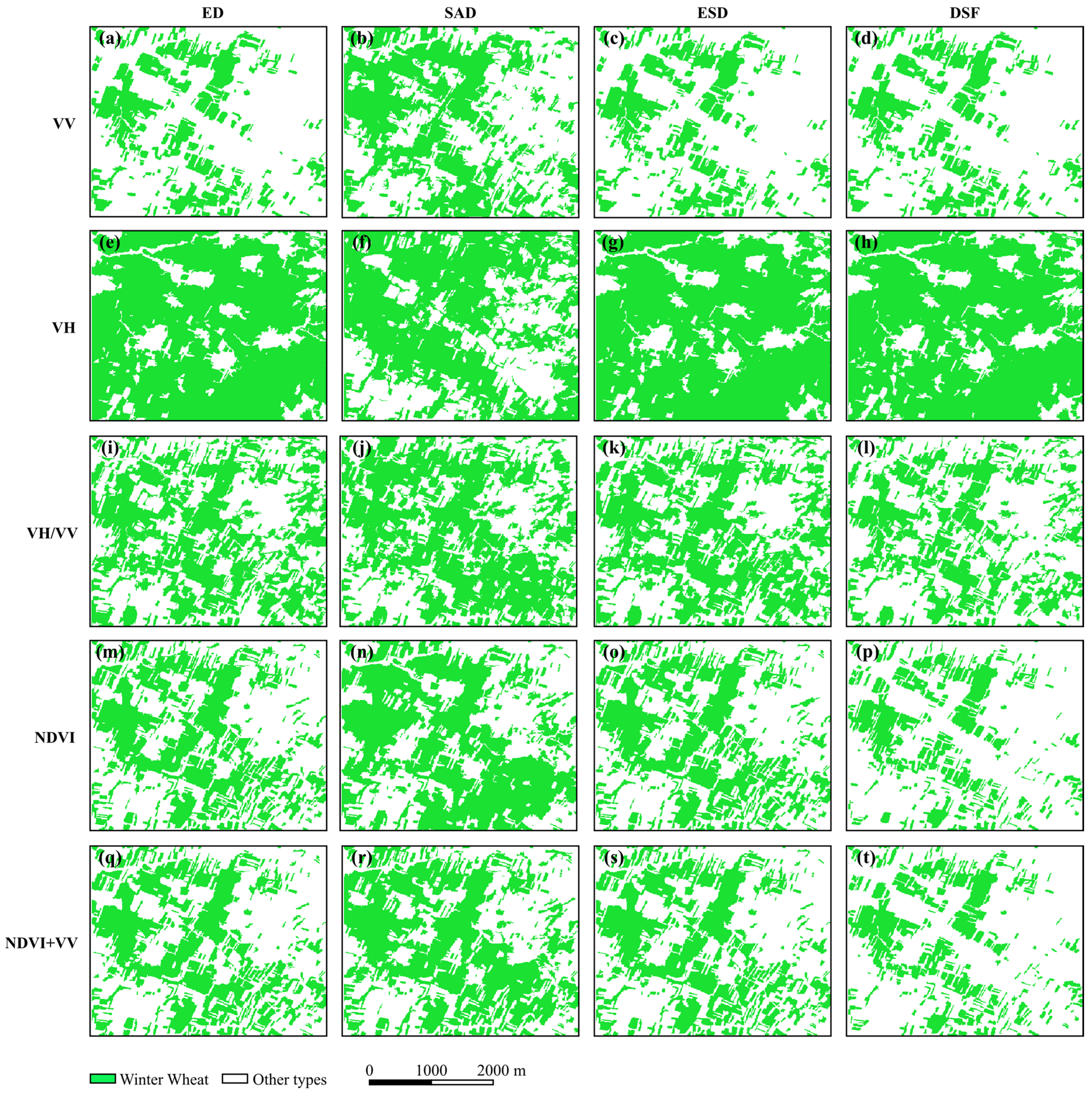
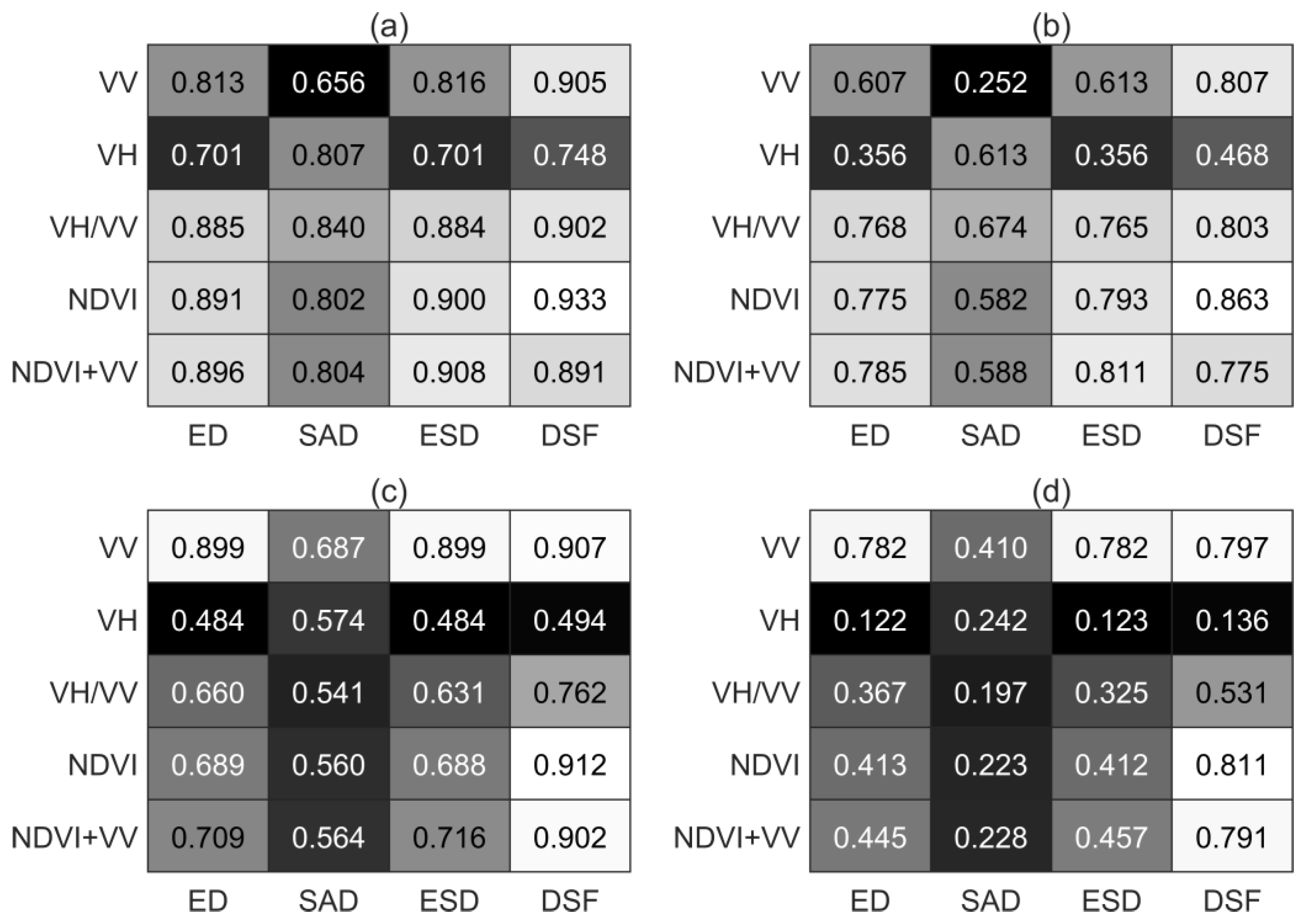
A new similarity measure (DSF) is introduced and achieves the best classification accuracy in all feature bands (e.g., NDVI, VV, VH/VV, NDVI + VV) and in both study sites. The new measure considers both distance difference and shape similarity, which can better describe the detailed differences between TPPs of land covers, thus obtaining better classification results. Generally speaking, different land covers often have different TPPs while the same land covers have the same TPPs. However, due to complicated biological and abiotic factors, the TPPs of specific ground objects often have unpredictable nonlinear distortion, resulting in the phenomena characterized by the ‘same object with a different spectrum’ and a ‘different object with the same spectrum’, which makes feature extraction and image interpretation difficult. Broad metrics may lead to a false alarm of target objects and thus result in overestimates, while strict metrics may lead to omissions of target objects, thus resulting in underestimates. Existing similarity measures have their advantages, and some focus on the distance difference while some focus on the shape similarity. Using a single measure to evaluate the correlation of two TPPs often results in great uncertainty in classification results. In particular, in large-scale areas, the differences in climate, soil, and topography lead to great variability in the TPPs of surface objects. Using a single distance or shape measure will inevitably lead to great deviation between the predicted results and the actual surface features.
Although some composite measures have been expected to solve the above problems, few of them are widely accepted and used. The reason for this is that these measures are only a simple addition or multiplication between existing single measures, lacking scientific explanation and sufficient practical proof. These measures may achieve good results in small specific test areas, but the generalization performance in time and space often cannot stand the test. In addition, the generalization ability of these similarity measures to different sensors, features, and bands is also a great challenge to their performance. Their performance varies with the input bands and features. When the TPPs of the same land cover type extracted from different sensors or different bands have considerable nonlinear variations, a qualified similarity measurement should be able to identify it and assign a consistent attribute label for it. If this is not practical, finding an optimal and robust similarity measure for each commonly used feature or band (e.g., NDVI, EVI, VV, VH) may be a good alternative. This issue will be further studied in our future work.
The SNIC segmentation adopted in this study is a kind of superpixel clustering segmentation algorithm, which has a simple principle and high time efficiency. The algorithm generally divides a large surface feature into several spatial objects with high homogeneity. It avoids including different surrounding parts across the boundary to ensure the consistent category attribute for each object and significantly reduces the segmentation error. In this study, the SNIC segmentation with the fusion of the S2 optical image and the S1 SAR image achieves satisfactory segmentation results, which provided highly homogenous spatial objects and perfect details. Most of the adjacent crops of different species in small areas or thin strip plots are well separated, indicating that the combined use of optical and SAR imagery has improved the separability of land covers. Although the SNIC algorithm does not need to input the optimal segmentation scale, it needs to determine the density of seed points, that is, the sampling interval of seed points. In this study, we use three sampling intervals (i.e., 10, 20, and 30 pixels) to generate seed points and implement the experiments under the three conditions. Finally, we find that the optimal sampling interval of seed points is 20 pixels. In this case, the segmentation algorithm not only derives the spatial objects with high homogeneity and consistent boundaries with actual ground features but also provides fine ground details. The object-based approach may not show significant advantages over pixel-level classification in small study areas, but it can provide an excellent solution to the problems caused by highly heterogeneous surfaces, mixed pixels, and image noise to significantly improve the accuracy and consistency of large scale classification.
This study found that different spectral or VI bands displayed different performances for land cover classification. These findings demonstrate that the ability of remote sensing to distinguish land cover types varies with bands. NDVI has more potent universality and shows excellent capability for distinguishing various land cover types. The NDVI band achieves the best overall classification accuracy, although it is very close to that of the NDVI + VV band. Surprisingly, the VV polarization of SAR imagery has produced impressive results over various land cover types that are very close to those of the NDVI band. The better performance of VV polarization in comparison with VH is because wheat plants have dominant vertical structure so that the VV-polarized backscattered energy is stronger than that from the VH-polarized signals [47]. As the growing season continues, the vertical structure of wheat plants changes greatly, and wheat shows a unique temporal phenology curve that is different from other land covers, which is beneficial to winter wheat identification [48]. In addition, VV polarization achieves such good winter wheat maps partly because of the speckle noise reduction by image segmentation. Based on segmented spatial objects, VV polarization displays outstanding capability in distinguishing winter wheat from other easily confused crops. This is very important for crop mapping with multitemporal remote sensing. Because of the cloudy weather, optical imagery may be unavailable during the crop growth period, which harms the temporal-phenology-based classification. In this case, SAR imagery is expected to provide trusted alternatives. Due to the complexity of the land surface composition and the mechanism for remote sensing imaging, a single band or feature is prone to failure when trying to solve all problems in most cases. Although the commonly used bands or features can be used as alternatives, they can only possibly produce the second-best classification results. Exploring the dominant bands or features for specific land cover types and using them for image interpretation would potentially improve the land cover and land use classifications in nature.

6. Conclusions

This study developed an automatic object-based approach for winter wheat mapping based on multitemporal optical and SAR imagery. The new DSF and ESD measures in winter wheat mapping were evaluated with ground truth data and compared with the commonly used ED and SAD measures. Additionally, the performance of optical and SAR imagery with various combinations of bands and measures was also evaluated. The results demonstrated that the DSF measure achieved the best classification results in all feasible bands, with higher precision and more details than other similarity measures. The classification results of ED in most bands were significantly better than those of SAD, indicating that the absolute distance difference was more important than shape similarity in assessing sample similarity. The ESD measurement achieved similar classification results to ED, and the classification accuracy was not significantly improved. In terms of band performance, the NDVI band showed a balanced performance in all land cover types and distinguished them very well. The overall accuracy of NDVI was better than the three polarization bands of the SAR image, while the VV polarization also displayed great potential for mapping winter wheat with the assistance of image segmentation. The fusion of optical and SAR imagery achieved better results in image segmentation and achieved evenly matched accuracy in winter wheat mapping compared to the best single data, indicating that the fusion of remote sensing data had great potential in image segmentation and classification. Overall, the developed approach worked well for winter wheat mapping and provided beneficial inspiration and new ideas for crop classification using multitemporal optical and SAR images.

Author Contributions

Conceptualization, Limei Wang and Guowang Jin; Methodology, Limei Wang; Software, Limei Wang; Validation, Limei Wang and Xin Xiong; Formal Analysis, Limei Wang; Investigation, Limei Wang and Hongmin Zhang; Resources, Guowang Jin and Hongmin Zhang; Data Curation, Limei Wang and Ke Wu; Writing-Original Draft Preparation, Limei Wang; Writing-Review & Editing, Limei Wang and Xin Xiong; Visualization, Limei Wang and Ke Wu; Supervision, Guowang Jin; Project Administration, Guowang Jin; Funding Acquisition, Guowang Jin. All authors have read and agreed to the published version of the manuscript.

Funding

This research was funded by the National Natural Science Foundation of China under Grants numbers 41474010 and 61401509.

Institutional Review Board Statement

Not applicable.

Informed Consent Statement

Not applicable.

Data Availability Statement

All data used in the research are openly available in the ESA archives (https://sentinel.esa.int/web/sentinel/home/, accessed on 21 July 2022) and within Google Earth Engine. The GEE codes developed in this research are available, upon any reasonable request, by emailing the authors.

Conflicts of Interest

The authors declare no conflict of interest.

References

  1. Chang, Y.F.; Wong, J.R. Regeneration of Plants from Protoplasts of Triticum aestivum L. (Wheat). In Plant Protoplasts and Genetic Engineering; Bajaj, Y.P.S., Ed.; Springer: Berlin/Heidelberg, Germany, 1994; Volume 29, pp. 161–171. [Google Scholar]
  2. Li, X.; Zheng, C.; Cao, C.; Dang, H.; Sun, J.; Li, K.; Ma, J. Analysis of Climatic Potential Productivity and Wheat Production in Different Producing Areas of the Northern Hemisphere. IOP Conf. Ser. Earth Environ. Sci. 2020, 427, 012010. [Google Scholar] [CrossRef]
  3. Hyles, J.; Bloomfield, M.T.; Hunt, J.R.; Trethowan, R.M.; Trevaskis, B. Phenology and Related Traits for Wheat Adaptation. Heredity 2020, 125, 417–430. [Google Scholar] [CrossRef] [PubMed]
  4. Urban, O.; Hlaváová, M.; Klem, K.; Novotná, K.; Rapantová, B.; Smutná, P.; Horáková, V.; Hlavinka, P.; Škarpa, P.; Trnka, M. Combined Effects of Drought and High Temperature on Photosynthetic Characteristics in Four Winter Wheat Genotypes. Field Crop. Res. 2018, 223, 137–149. [Google Scholar] [CrossRef]
  5. Tian, J.; Zhu, X.; Shen, Z.; Wu, J.; Wang, J. Investigating the Urban-Induced Microclimate Effects on Winter Wheat Spring Phenology Using Sentinel-2 Time Series. Agric. Forest Meteorol. 2020, 294, 108153. [Google Scholar] [CrossRef]
  6. G’Oes, C.; Bekkers, E. The Impact of Geopolitical Conflicts on Trade, Growth, and Innovation. arXiv 2022, arXiv:2203.121732. [Google Scholar]
  7. Gong, Y. A Soil Layered Water Budget Model for Winter Wheat and Summer Maize. Acta Agric. Univ. Pekin. 1995, 1, 61–67. [Google Scholar]
  8. Pique, G.; Wijmert, T.; Fieuzal, R.; Ceschia, E. Estimation of Crop Production and CO2 Fluxes Using Remote Sensing: Application to a Winter Wheat/Sunflower Rotation. Environ. Sci. Proc. 2021, 4, 15. [Google Scholar]
  9. Deb, S.; Bhadoria, P.; Mandal, B.; Rakshit, A.; Singh, H.B. Soil Organic Carbon: Towards Better Soil Health, Productivity and Climate Change Mitigation. Clim. Chang. Environ. Sustain. 2015, 3, 26–34. [Google Scholar] [CrossRef]
  10. Simonneaux, V.; Duchemin, B.; Helson, D.; Er-Raki, S.; Olioso, A.; Chehbouni, A.G. The Use of High-Resolution Image Time Series for Crop Classification and Evapotranspiration Estimate over an Irrigated Area in Central Morocco. Int. J. Remote Sens. 2008, 29, 95–116. [Google Scholar] [CrossRef] [Green Version]
  11. Walker, J.J.; de Beurs, K.M.; Henebry, G.M. Land Surface Phenology along Urban to Rural Gradients in the U.S. Great Plains. Remote Sens. Environ. 2015, 165, 42–52. [Google Scholar] [CrossRef]
  12. Zhang, G.; Xiao, X.; Dong, J.; Kou, W.; Jin, C.; Qin, Y.; Zhou, Y.; Wang, J.; Menargu, M.A.; Biradard, C. Mapping Paddy Rice Planting Areas Through Time Series Analysis of MODIS Land Surface Temperature and Vegetation Index Data. ISPRS J. Photogramm. Remote Sens. 2016, 106, 157–171. [Google Scholar] [CrossRef] [PubMed] [Green Version]
  13. Zhong, L.; Hu, L.; Yu, L.; Gong, P.; Biging, G.S. Automated Mapping of Soybean and Corn Using Phenology. ISPRS J. Photogramm. Remote Sens. 2016, 119, 151–164. [Google Scholar] [CrossRef] [Green Version]
  14. Zhang, M.; Zhou, Q.; Chen, Z.; Jia, L.; Zhou, Y.; Cai, C. Crop Discrimination in Northern China with Double Cropping Systems using Fourier Analysis of Time-Series MODIS Data. Int. J. Appl. Earth Observ. Geoinform. 2008, 10, 476–485. [Google Scholar]
  15. Kocian, A.; Carmassi, G.; Cela, F.; Incrocci, L.; Milazzo, P.; Chessa, S. Bayesian Sigmoid-type Time Series Forecasting with Missing Data for Greenhouse Crops. Sensors 2020, 20, 3246. [Google Scholar] [CrossRef] [PubMed]
  16. Caballero, G.R.; Platzeck, G.; Pezzola, A.; Casella, A.; Delegido, J. Assessment of Multi-Date Sentinel-1 Polarizations and GLCM Texture Features Capacity for Onion and Sunflower Classification in an Irrigated Valley: An Object Level Approach. Agronomy 2020, 10, 845. [Google Scholar] [CrossRef]
  17. Muthukumarasamy, I.; Shanmugam, R.S.; Usha, T. Incorporation of Textural Information with SAR and Optical Imagery for Improved Land Cover Mapping. Environ. Earth Sci. 2019, 78, 643. [Google Scholar] [CrossRef]
  18. Chureesampant, K.; Susaki, J. Multi-temporal SAR and Optical Data Fusion with Texture Measures for Landcover Classification Based on the Bayesian Theory. ISPRS. SC. Newlett. 2008, 5, 1183–1188. [Google Scholar]
  19. Luo, C.; Qi, B.; Liu, H.; Guo, D.; Shao, Y. Using Time Series Sentinel-1 Images for Object-Oriented Crop Classification in Google Earth Engine. Remote Sens. 2021, 13, 561. [Google Scholar] [CrossRef]
  20. Jiao, X.; Kovacs, J.M.; Shang, J.; Mcnairn, H.; Walters, D.; Ma, B.; Geng, X. Object-Oriented Crop Mapping and Monitoring using Multi-Temporal Polarimetric Radarsat-2 Data. ISPRS J. Photogramm. Remote Sens. 2014, 96, 38–46. [Google Scholar] [CrossRef]
  21. Tassi, A.; Gigante, D.; Modica, G.; Di Martino, L.; Vizzari, M. Pixel- vs. Object-Based Landsat 8 Data Classification in Google Earth Engine Using Random Forest: The Case Study of Maiella National Park. Remote Sens. 2021, 13, 2299. [Google Scholar] [CrossRef]
  22. Yang, G.; Yu, W.; Yao, X.; Zheng, H.; Cao, Q.; Zhu, Y.; Cao, W.; Cheng, T. AGTOC: A Novel Approach to Winter Wheat Mapping by Automatic Generation of Training Samples and One-Class Classification on Google Earth Engine. Int. J. Appl. Earth Observ. Geoinform. 2021, 102, 102446. [Google Scholar] [CrossRef]
  23. Sheykhmousa, M.; Mahdianpari, M. Support Vector Machine Versus Random Forest for Remote Sensing Image Classification: A Meta–Analysis And Systematic Review. IEEE J. Sel. Topics Appl. Earth Obs. Remote Sens. 2020, 13, 6308–6325. [Google Scholar] [CrossRef]
  24. Cho, M.A.; Debba, P.; Mathieu, R.; Naidoo, L.; Aardt, J.V.; Asner, G.P. Improving Discrimination of Savanna Tree Species Through a Multiple-Endmember Spectral Angle Mapper Approach: Canopy-Level Analysis. IEEE Trans. Geosci. Remote Sens. 2010, 48, 4133–4142. [Google Scholar] [CrossRef]
  25. Verrelst, J. Classification of Plant Ecological Units in Heterogeneous Semi-Steppe Rangelands: Performance Assessment of Four Classification Algorithms. Remote Sens. 2021, 13, 3433. [Google Scholar]
  26. Abbas, A.W.; Minallh, N.; Ahmad, N.; Abid, S.; Khan, M. K-Means and ISODATA Clustering Algorithms for Landcover Classification using Remote Sensing. Sindh Univ. Res. J. 2016, 48, 315–318. [Google Scholar]
  27. Zhang, L.; Weng, Q.; Shao, Z. An Evaluation of Monthly Impervious Surface Dynamics by Fusing Landsat and MODIS Time Series in the Pearl River Delta, China, from 2000 To 2015. Remote Sens. Environ. 2017, 201, 99–114. [Google Scholar] [CrossRef]
  28. Xu, Y.; Yu, L.; Zhao, F.; Cai, X.; Zhao, J.; Lu, H.; Gong, P. Tracking Annual Cropland Changes from 1984 to 2016 using Time-Series Landsat Images with a Change-Detection and Post-Classification Approach: Experiments from Three Sites in Africa. Remote Sens. Environ. 2018, 218, 13–31. [Google Scholar] [CrossRef]
  29. Xu, L.; Zhang, H.; Wang, C.; Zhang, B.; Liu, M. Crop Classification Based on Temporal Information using Sentinel-1 SAR Time-Series Data. Remote Sens. 2018, 11, 53. [Google Scholar] [CrossRef] [Green Version]
  30. Vizilter, Y.V.; Zheltov, S.Y. Similarity Measures and Comparison Metrics for Image Shapes. J. Comput. Syst. Sci. Int. 2014, 53, 542–555. [Google Scholar] [CrossRef]
  31. Mimmack, G.M.; Mason, S.J.; Galpin, J.S. Choice of Distance Matrices in Cluster Analysis: Defining Regions. J. Clim. 2010, 14, 2790–2797. [Google Scholar] [CrossRef]
  32. Modh, J.S.; Brijesh, S.; Satish, S.K. A New K-mean Color Image Segmentation with Cosine Distance for Satellite Images. IJEAT 2012, 1, 27–30. [Google Scholar]
  33. Hao, P.; Zhan, Y.; Wang, L.; Niu, Z.; Shakir, M. Feature Selection of Time Series MODIS Data for Early Crop Classification using Random Forest: A Case Study in Kansas, USA. Remote Sens. 2015, 7, 5347–5369. [Google Scholar] [CrossRef] [Green Version]
  34. Chakhar, A.; Ortega-Terol, D.; Hernández-López, D.; Ballesteros, R.; Moreno, M.A. Assessing the Accuracy of Multiple Classification Algorithms for Crop Classification using Landsat-8 and Sentinel-2 Data. Remote Sens. 2020, 12, 1735. [Google Scholar] [CrossRef]
  35. Ma, Z.; Liu, Z.; Zhao, Y.; Zhang, L.; Li, S. An Unsupervised Crop Classification Method Based on Principal Components Isometric Binning. ISPRS J. Photogramm. Remote Sens. 2020, 9, 648. [Google Scholar] [CrossRef]
  36. Zhao, N. Integration of Sentinel 1 and Sentinel 2 Satellite Images for Crop Mapping. Appl. Sci. 2021, 11, 10104. [Google Scholar]
  37. Mcnairn, H.; Shang, J.; Champagne, C.; Jiao, X. Terrasar-X and Radarsat-2 for Crop Classification and Acreage Estimation. IGARSS 2009, 2, 11150411. [Google Scholar]
  38. Zhang, X.; Liu, J.F.; Qin, Z.; Qin, F. Winter Wheat Identification by Integrating Spectral and Temporal Information Derived from Multi-Resolution Remote Sensing Data. J. Integr. Agr. 2019, 18, 2628–2643. [Google Scholar] [CrossRef]
  39. Zuo, X.; Han, L.; Ge, Q.; Zhang, Z.; Tian, J. Area Extraction and Interannual Variation Monitoring of Winter Wheat in Counties Based on GF-1 Satellite. J. Henan Univ. (Nat. Sci.) 2019, 49, 9. [Google Scholar]
  40. Li, C.; Chen, W.; Wang, Y.; Wang, Y.; Ma, C.; Li, Y.; Li, J.; Zhai, W. Mapping Winter Wheat with Optical and SAR Images Based on Google Earth Engine in Henan Province, China. Remote Sens. 2022, 14, 284. [Google Scholar] [CrossRef]
  41. Tao, J.B.; Wen-Bin, W.U.; Zhou, Y.; Wang, Y.; Jiang, Y. Mapping Winter Wheat Using Phenological Feature of Peak Before Winter on the North China Plain Based on Time-Series MODIS Data. J. Integr. Agr. 2017, 16, 348–359. [Google Scholar] [CrossRef] [Green Version]
  42. Zhou, T.; Pan, J.; Han, T.; Wei, S. Planting Area Extraction of Winter Wheat Based on Multi-Temporal SAR Data and Optical Imagery. Trans. CSAE 2017, 33, 7. [Google Scholar]
  43. Mullissa, A.; Vollrath, A.; OdongoBraun, C.; Slagter, B.; Balling, J.; Gou, Y.; Gorelick, N.; Reiche, J. Sentinel-1 SAR Backscatter Analysis Ready Data Preparation in Google Earth Engine. Remote Sens. 2021, 13, 1954. [Google Scholar] [CrossRef]
  44. Achanta, R.; Susstrunk, S. Superpixels and Polygons using Simple Non-Iterative Clustering. In Proceedings of the 2017 IEEE Conference on Computer Vision and Pattern Recognition (CVPR), Honolulu, HI, USA, 21–26 July 2017; pp. 4895–4904. [Google Scholar]
  45. Yang, L.; Wang, L.; Abubakar, G.A.; Huang, J. High-Resolution Rice Mapping Based on SNIC Segmentation and Multi-Source Remote Sensing Images. Remote Sens. 2021, 13, 1148. [Google Scholar] [CrossRef]
  46. Zxa, B.; Msb, C.; Msb, C.; Ga, D. Estimators and Confidence Intervals of f2 Using Bootstrap Methodology for the Comparison of Dissolution Profiles. Comput. Meth. Prog. Biomed. 2021, 212, 106449. [Google Scholar]
  47. Hajj, M.E.; Baghdadi, N.; Bazzi, H.; Zribi, M. Penetration Analysis of SAR Signals in the C And L Bands for Wheat, Maize, and Grasslands. Remote Sens. 2019, 11, 31. [Google Scholar] [CrossRef] [Green Version]
  48. Yan, W.; Zhang, Y.; Yang, T.; Liu, X. A Microwave Scattering Model for Simulating the C-Band SAR Backscatter of Wheat Canopy. Ame. J. Remote Sens. 2019, 7, 13–24. [Google Scholar] [CrossRef] [Green Version]
Figure 1. Location of the study sites and the ground truth: (a) Location of the two sites; (b,d) The ground truth samples overlayed on a false-color composite image (Red: NIR, Green: Red, Blue: Green), and (c,e) the ground truth parcels of main land cover types.
Ijgi 11 00424 g001
Figure 2. Flow chart of this study.
Ijgi 11 00424 g002
Figure 3. Flow chart of remote sensing image preprocessing.
Ijgi 11 00424 g003
Figure 4. The false-color composite S2 imagery: before (a) and after pansharpening (b) in Site 1; before (c) and after pansharpening (d) in Site 2. The false-color composite: R: B5-vegetation red edge1, G: B8A-NIR1, B: B12-SWIR2.
Ijgi 11 00424 g004
Figure 5. Monthly composite images of S1 imagery in March 2020: (a) VV polarization on 15 March in Site 1; (b) monthly composite VV polarization in Site 1; (c) VV polarization on March 18 in Site 2; (d) monthly composite VV polarization in Site 2.
Ijgi 11 00424 g005
Figure 6. Temporal phenology patterns of VV (a), VH (b), VH/VV (c) and NDVI (d) bands for winter wheat and typical land cover types derived from multitemporal S2 and S1 imagery over the winter wheat season of 2019–2020 (Note: WW1 and WW2: winter wheat, BU: built-up, EW: evergreen woodland, WB: water body, UP: unsown peanut, DW: deciduous woodland, OR: orchard, WR: winter rapeseed.).
Ijgi 11 00424 g006
Figure 7. Segmentation results with the SNIC algorithm superimposed over the monthly composite S2 subset imagery of March 2020 in false color in Site 1: (a) segmented by S2_202003 input bands; (b) segmented by the S2_15DAY NDVI time series; (c) segmented by S1_202003 input bands; (d) segmented by S1_202003_GLCM input bands; (e) segmented by S1S2_202003 input bands. The description of the input imagery and the corresponding input bands for the SNIC algorithm are shown in Table 4. The false-color composite of the images is shown in Figure 1.
Ijgi 11 00424 g007
Figure 8. Classification maps from each combination of similarity measures and bands in Site 1: (ad) VV_ED, VV_SAD, VV_ESD, VV_DSF; (eh) VH_ED, VH_SAD, VH_ESD, VH_DSF; (il) VH/VV_ED, VH/VV_SAD, VH/VV_ESD, VH/VV_DSF; (mp) NDVI_ED, NDVI_SAD, NDVI_ESD, NDVI_DSF; (qt) NDVI + VV_ED, NDVI + VV_SAD, NDVI + VV_ESD, NDVI + VV_DSF.
Ijgi 11 00424 g008
Figure 9. Classification maps from each combination of similarity measures and bands in Site 2: (ad) VV_ED, VV_SAD, VV_ESD, VV_DSF; (eh) VH_ED, VH_SAD, VH_ESD, VH_DSF; (il) VH/VV_ED, VH/VV_SAD, VH/VV_ESD, VH/VV_DSF; (mp) NDVI_ED, NDVI_SAD, NDVI_ESD, NDVI_DSF; (qt) NDVI + VV_ED, NDVI + VV_SAD, NDVI + VV_ESD, NDVI + VV_DSF.
Ijgi 11 00424 g009
Figure 10. The false-color composite of S2 subset images over typical orchard, lotus pond and built-up (a), evergreen woodland (e), and winter rapeseed sites (i,m); and the corresponding classification details of VV_DSF (b,f,j,n), NDVI_DSF (c,g,k,o) and NDVI + VV_DSF (d,h,l,p). The false-color composite of the images is shown in Figure 1.
Ijgi 11 00424 g010
Figure 11. Classification accuracy with each combination of bands and similarity measures in both study sites: (a) OA of Site 1; (b) Kappa of Site 1; (c) OA of Site 2; (d) Kappa of Site 2.
Ijgi 11 00424 g011
Figure 12. Rank of the classification accuracy with each combination of bands and similarity measures in both study sites: (a) OA of Site 1; (b) Kappa of Site 1; (c) OA of Site 2; (d) Kappa of Site 2.
Ijgi 11 00424 g012
Table 1. Photos of representative land cover types taken during the field survey.
DateWinter WheatWinter RapeseedUnsown PeanutOrchardWoodland
15 March Ijgi 11 00424 i001 Ijgi 11 00424 i002 Ijgi 11 00424 i003 Ijgi 11 00424 i004 Ijgi 11 00424 i005
5 April Ijgi 11 00424 i006 Ijgi 11 00424 i007 Ijgi 11 00424 i008 Ijgi 11 00424 i009 Ijgi 11 00424 i010
19 April Ijgi 11 00424 i011 Ijgi 11 00424 i012 Ijgi 11 00424 i013 Ijgi 11 00424 i014 Ijgi 11 00424 i015
Table 2. Description of preprocessed S1 and S2 imagery at pixel level.
DatasetsOriginal BandsDerived Bands
S1_15DAYVV, VHVH/VV, gray_asm, gray_contrast, gray_corr, gray_ent, gray_var, gray_idm, gray_savg
S2_15DAYB2, Blue; B3; Green; B4; Red; B5; Vegetation red edge 1; B6; Vegetation red edge 2; B7; Vegetation red edge 3; B8; Near Infrared1 (NIR1); B8A; Narrow near infrared (NIR2); B11; Short wave infrared 1 (SWIR1); B12; Short wave infrared 2 (SWIR2)NDVI; mNDWI; LSWI; EVI; BSI
Table 3. Vegetation indices calculated from Sentinel-2 imagery.
VIsDescriptionEquations
NDVINormalized difference vegetation index ( ρ B 8 ρ B 4 ) / ( ρ B 8 + ρ B 4 )
mNDWIModified normalized difference water index ( ρ B 3 ρ B 11 ) / ( ρ B 3 + ρ B 11 )
EVIEnhanced vegetation index 2.5 ( ρ B 8 ρ B 4 ) / ( 1 + ρ B 8 + 6 ρ B 4 7.5 ρ B 2 )
LSWILand surface water index ( ρ B 8 ρ B 11 ) / ( ρ B 8 + ρ B 11 )
BSIBare soil index ( ρ B 4 + ρ B 11 ) ( ρ B 8 + ρ B 2 ) ( ρ B 4 + ρ B 11 ) + ( ρ B 8 + ρ B 2 )
ρ is the surface reflectance of Sentinel-2 imagery, and the band names for Sentinel-2 imagery are reported in Table 2.
Table 4. Input imagery and the corresponding bands for SNIC segmentation.
Input ImageryInput Bands
S2_202003B2, B3, B4, B5, B8, B11, NDVI, LSWI, EVI, BSI
S2_15DAYNDVI
S1_202003VV, VH, VH/VV
S1_202003_GLCMVV, VH, VH/VV, gray_asm, gray_contrast, gray_corr, gray_ent, gray_var, gray_idm, gray_savg
S1S2_202003B2, B3, B4, B5, B8, B11, B12, VV, VH, VH/VV
Publisher’s Note: MDPI stays neutral with regard to jurisdictional claims in published maps and institutional affiliations.

