
Geocomputational Approach to Simulate and Understand the Spatial Dynamics of COVID-19 Spread in the City of Montreal, QC, Canada


Abstract
:1. Introduction
2. Materials and Methods
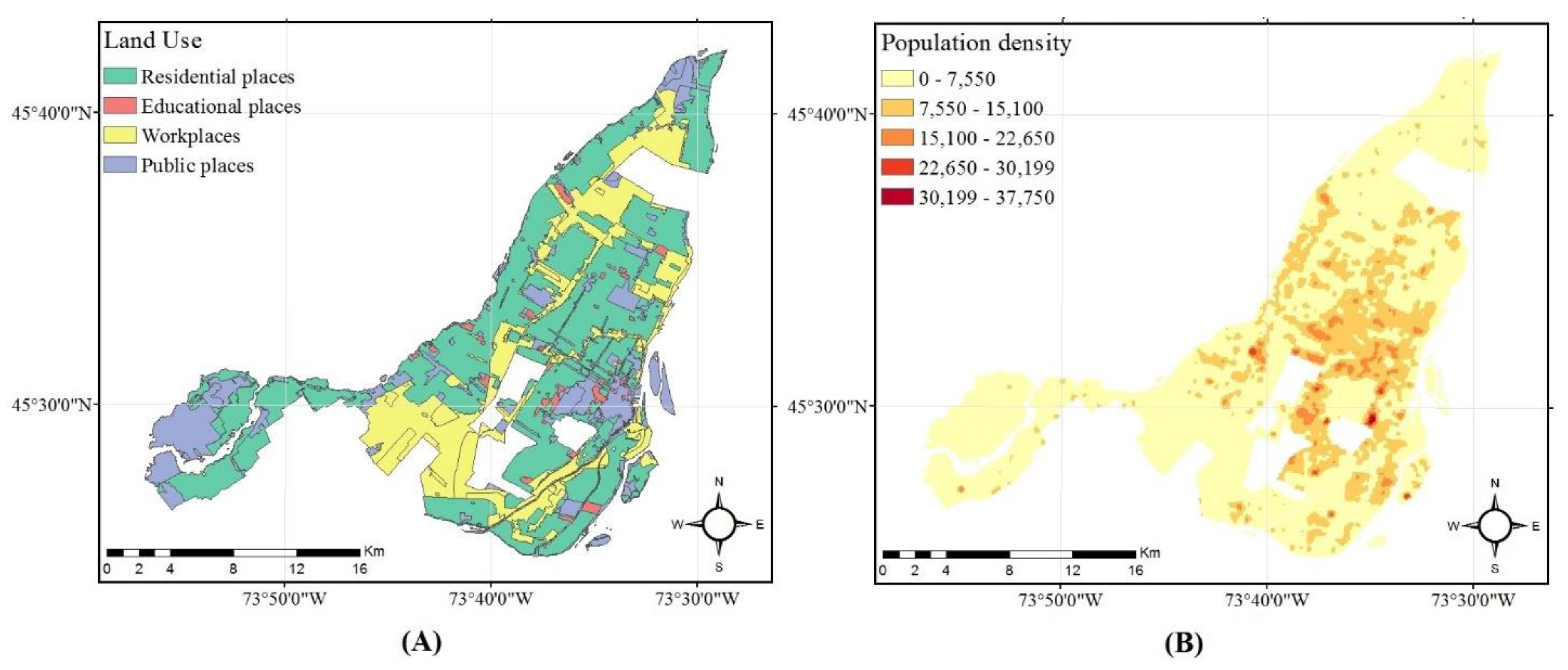
2.1. Overview of the Area under Study
2.2. Data and Preprocessing of the Input Data
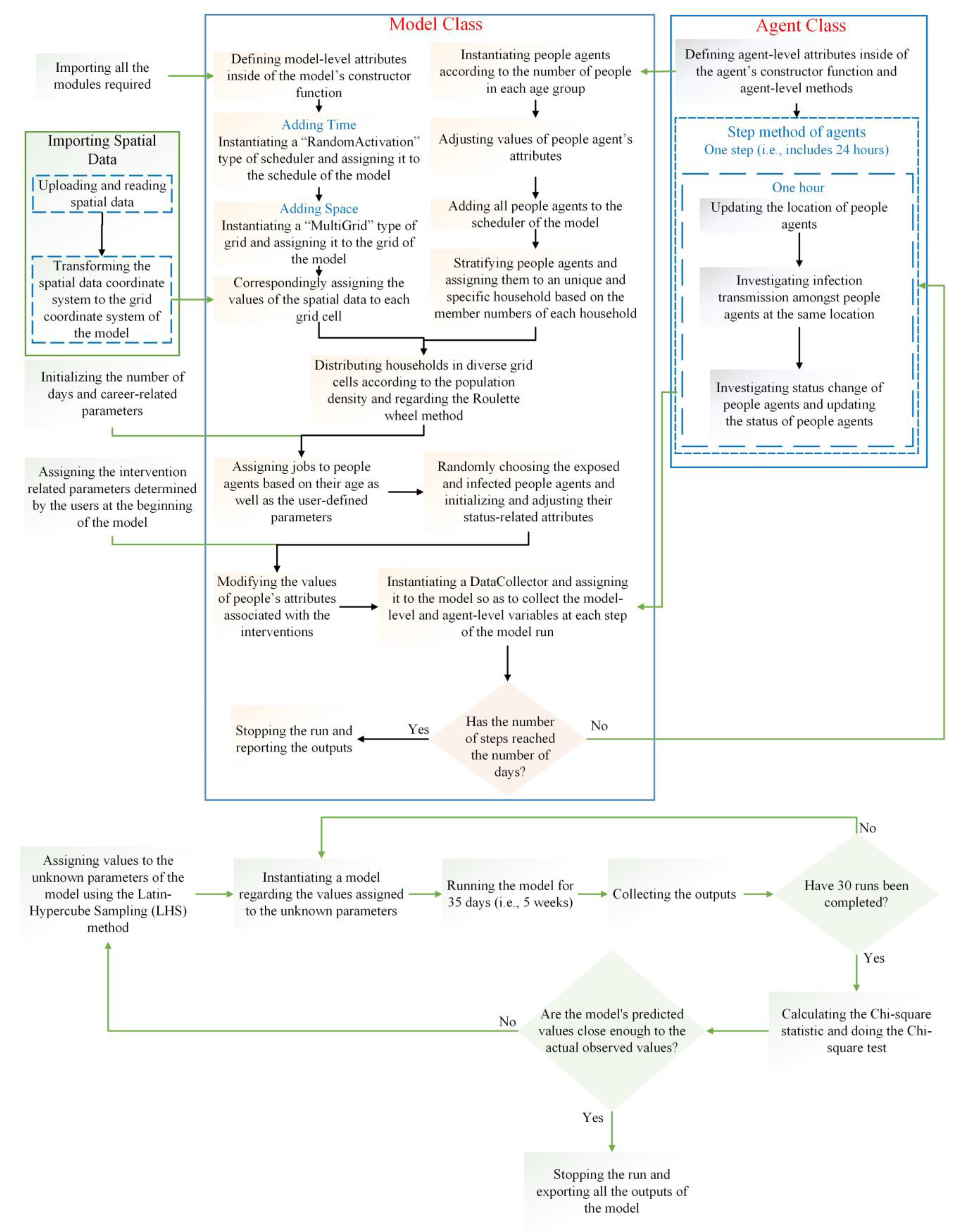
2.3. The Proposed Agent-Based Model
2.3.1. Model Overview
Purpose
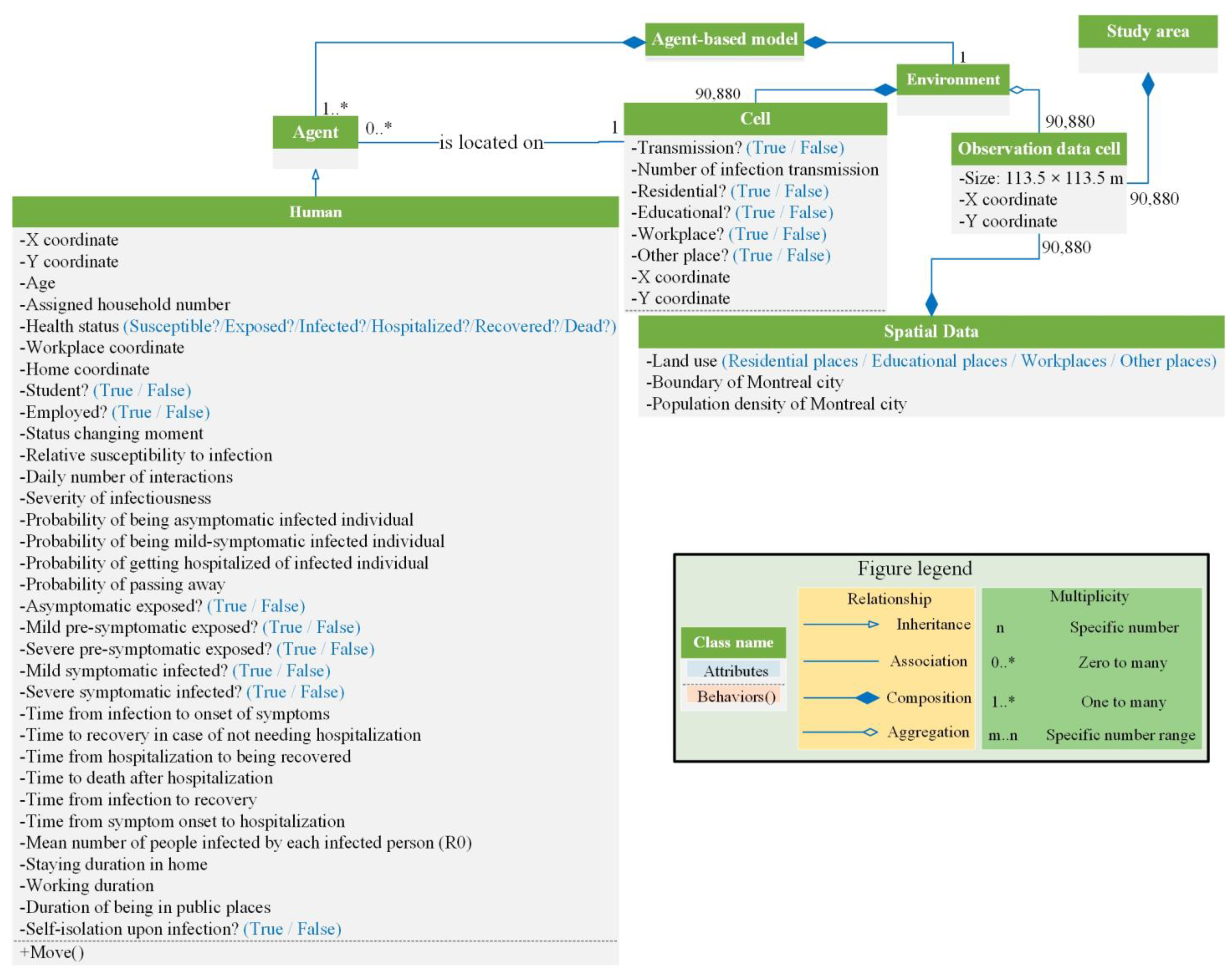
State Variables and Scales
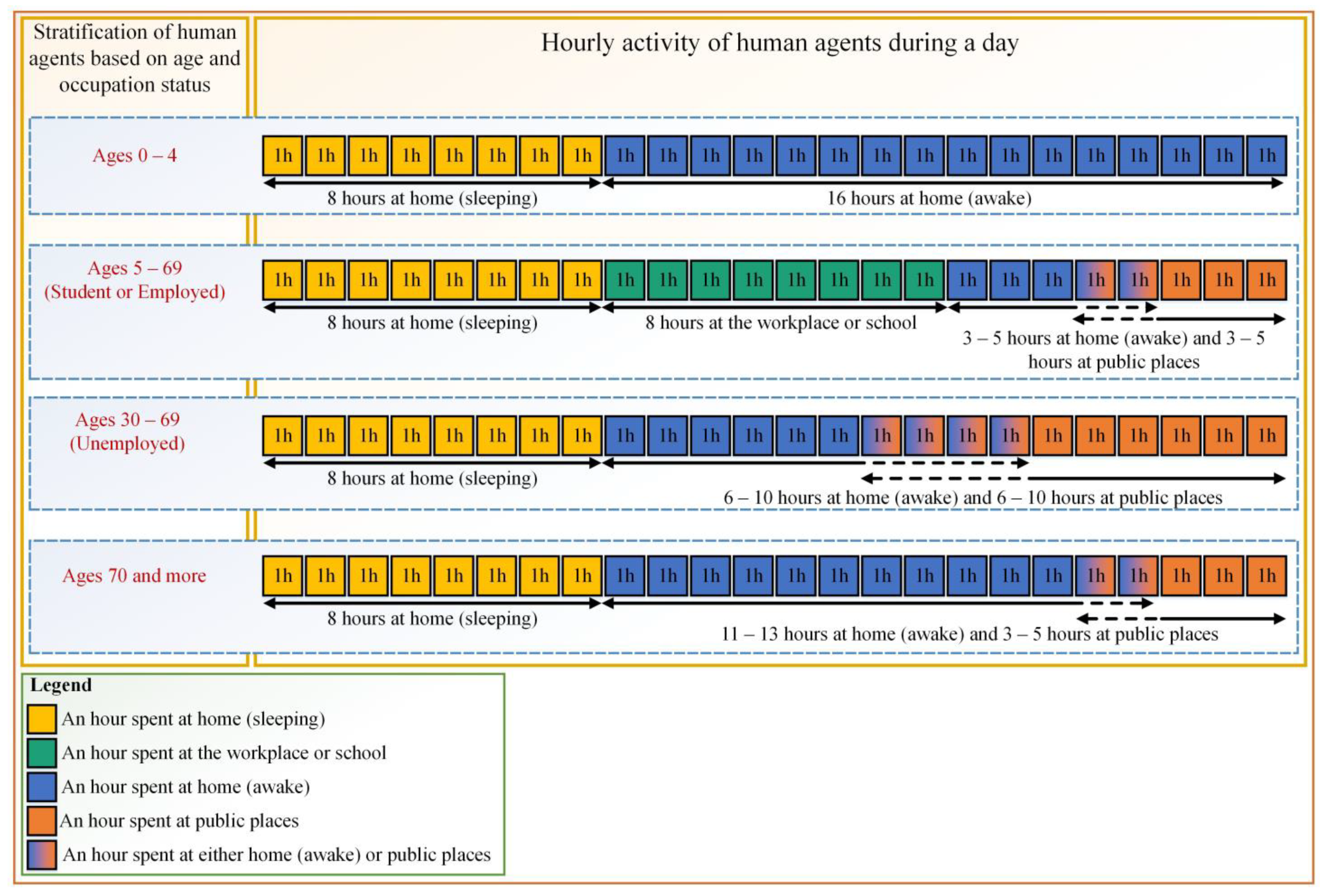
Process Overview and Scheduling
2.3.2. Design Concepts
Sensing
Interactions
Stochasticity
2.3.3. Details
Initialization
Input Data
Submodels
The Spatially Xplicit Environment
Agents
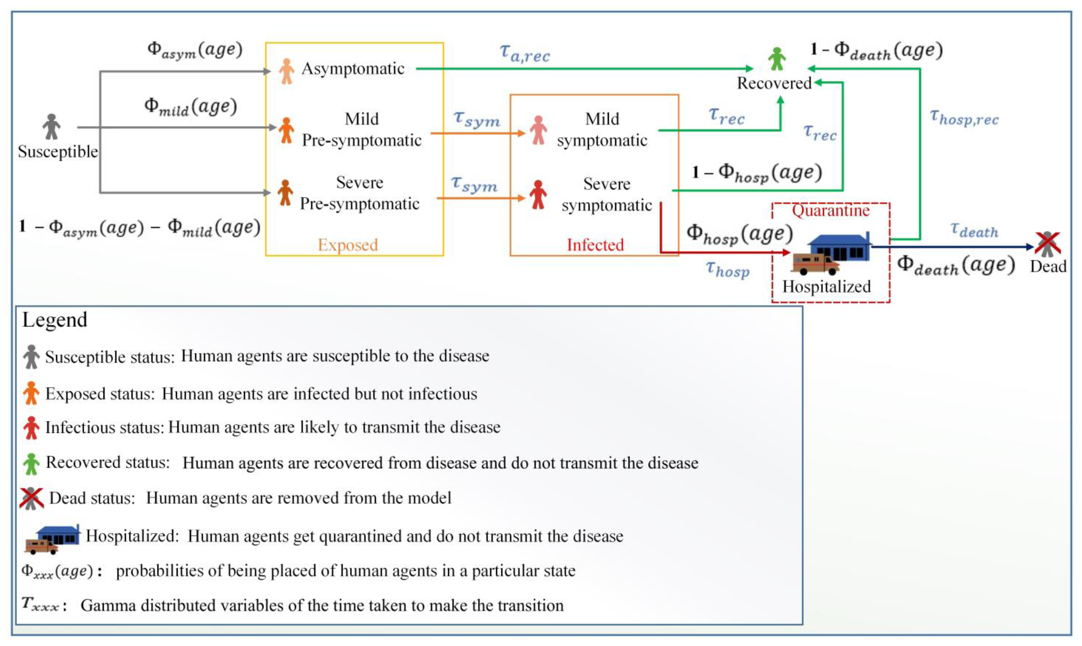
The Epidemiological Submodel
Control Interventions
2.3.4. Verification Process
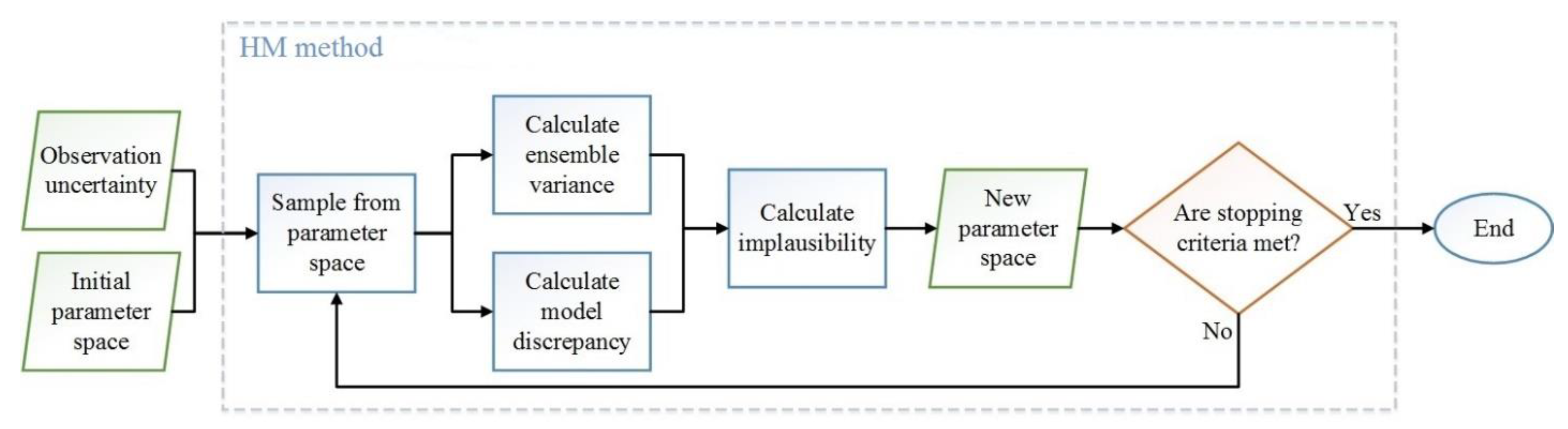
2.3.5. Calibration and Validation
3. Results
3.1. Model Verification
3.2. Model Calibration and Validation
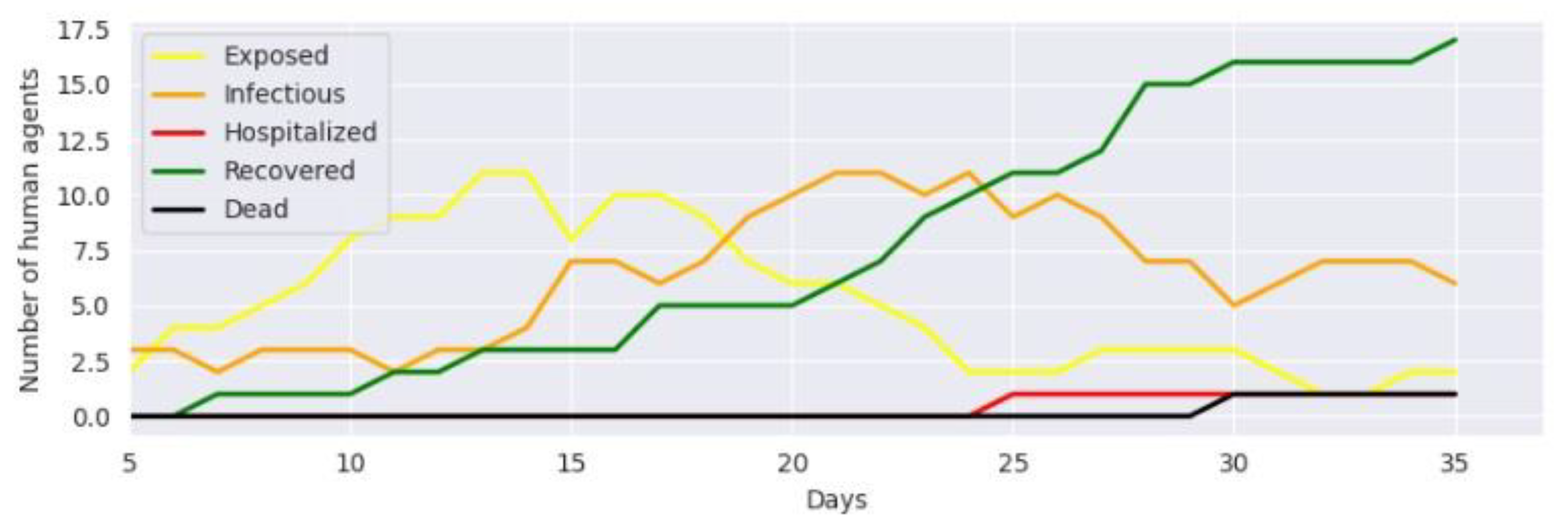
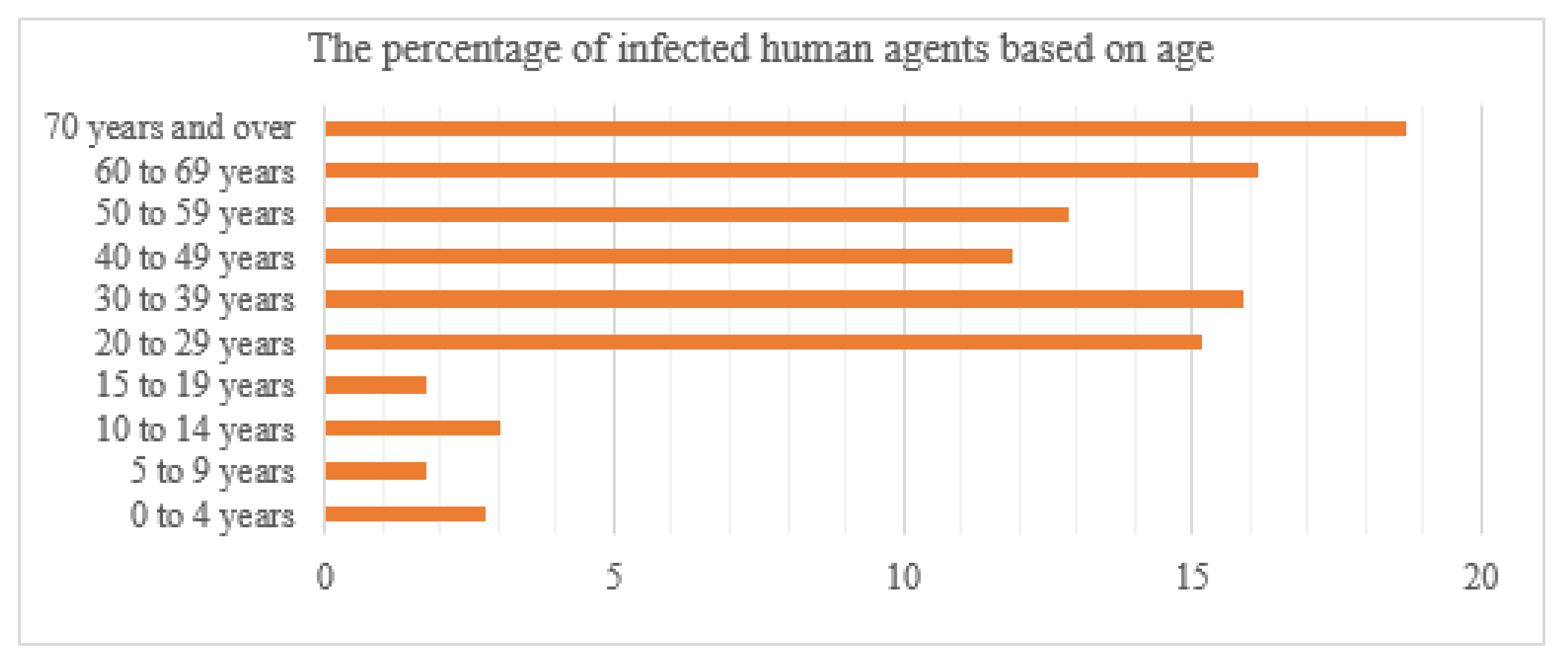
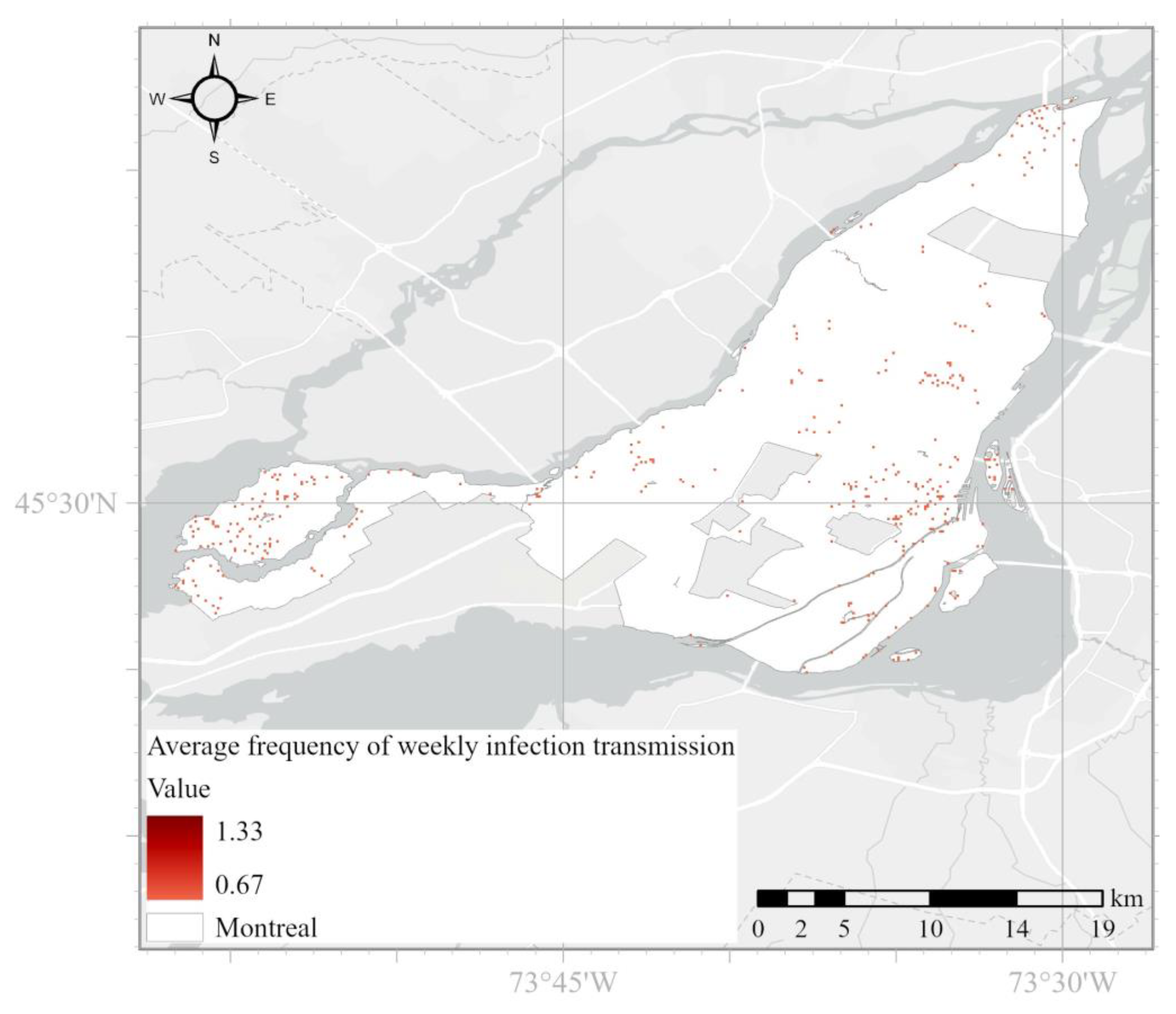
3.3. Model Outputs
3.4. Investigating the Number of Infected Human Agents in Case of Employing COVID-19 Control Interventions
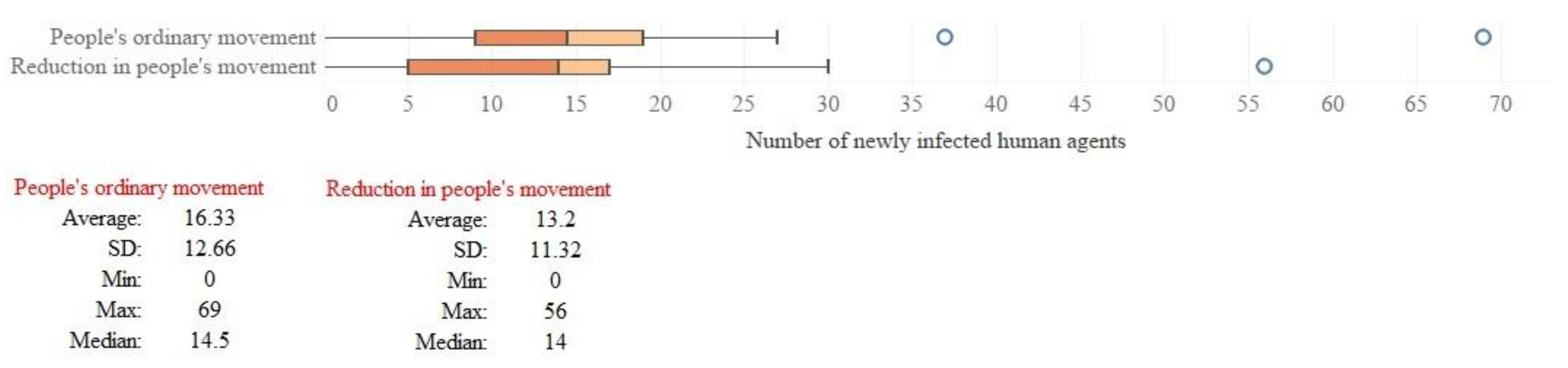
3.4.1. Reduction in Human-Mobility
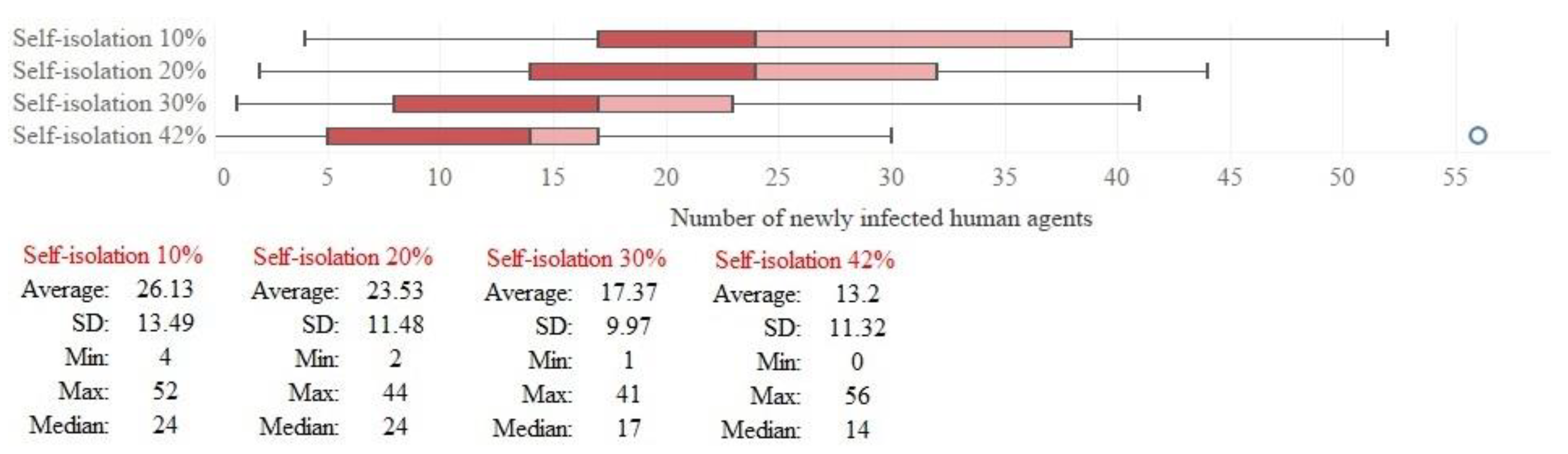
3.4.2. Self-Isolation Intervention
4. Discussion
5. Conclusions
Author Contributions
Funding
Data Availability Statement
Acknowledgments
Conflicts of Interest
Appendix A

| Age Range | Agent Number (Each Agent Represents 10 People in the Real World) | Population (in 2016) | Percentage (%) |
|---|---|---|---|
| 0 to 4 Years | 10,991 | 109,910 | 5.8% |
| 5 to 9 Years | 10,044 | 100,435 | 5.3% |
| 10 to 14 Years | 8528 | 85,275 | 4.5% |
| 15 to 19 Years | 9096 | 90,960 | 4.8% |
| 20 to 29 Years | 29,751 | 297,515 | 15.7% |
| 30 to 39 Years | 30,699 | 306,990 | 16.2% |
| 40 to 49 Years | 24,824 | 248,245 | 13.1% |
| 50 to 59 Years | 24,824 | 248,245 | 13.1% |
| 60 to 69 Years | 19,329 | 193,290 | 10.2% |
| 70 Years and over | 21,414 | 214,135 | 11.3% |
| Total | 189,500 | 1,895,000 | 100% |
| Household’s Size | Number of Households | Population | Population (Based on Agents) | Number of Households (Based on Agent) |
|---|---|---|---|---|
| 1 person | 342,510 (39.12%) | 342,510 | 34,251 | 34,251 |
| 2 persons | 259,295 (29.62%) | 518,590 | 51,860 | 25,930 |
| 3 persons | 118,645 (13.55%) | 355,935 | 35,592 | 11,864 |
| 4 persons | 97,490 (11.13%) | 389,960 | 38,996 | 9749 |
| 5 persons and more | 57,601(6.58%) | 288,005 | 28,800 | 5760 |
| Total | 875,541 | 1,895,000 | 189,499 | 87,554 |
| People | Number (Real World) | Agent Number | Percentage | |
|---|---|---|---|---|
| Employed | Employee | 810,955 | 81,096 | 50.71% |
| Self-employed | 231,580 | 23,158 | 14.48% | |
| Unemployed | 91,645 | 9164 | 5.73% | |
| Students (70% of people with 15–29 years of age) | 271,932 | 27,193 | 17% | |
| Not determined | 193,268 | 19,327 | 12.08% | |
| Total population of 15 years and over | 1,599,380 | 159,938 | 100% | |
Appendix B

Appendix C
| Parameters | Symbol | Value | Resources |
|---|---|---|---|
| Mean of the infectious period | 5.5 days | Ferretti et al., 2020 [67]; Hinch et al., 2021 [36] | |
| The standard deviation of the infectious period | 2.14 days | ||
| Mean number of people infected by each infected person | 4.5 | Ke et al., 2021 [38] | |
| Infectious rate of asymptomatic individuals relative to severely symptomatic individuals | 0.33 | Hinch et al., 2021 [36] | |
| Infectious rate of mildly symptomatic individuals relative to severely symptomatic individuals | 0.72 | Hinch et al., 2021 [36] | |
| Relative susceptibility of recipient to infection based on age | 0.35 | Zhang et al., 2020 [68] | |
| 0.69 | |||
| 1.03 | |||
| 1.03 | |||
| 1.03 | |||
| 1.03 | |||
| 1.27 | |||
| 1.52 |
Appendix D
| Age Range | Daily Number of Interactions, Normal Distribution with Mean (Standard Deviation) |
|---|---|
| 0–4 | 10.21 (7.65) |
| 5–9 | 14.81 (10.09) |
| 10–14 | 18.22 (12.27) |
| 15–19 | 17.58 (12.03) |
| 20–29 | 13.57 (10.6) |
| 30–39 | 14.14 (10.15) |
| 40–49 | 13.83 (10.86) |
| 50–59 | 12.30 (10.23) |
| 60–69 | 9.21 (7.96) |
| 70+ | 6.89 (5.83) |
References
- Ali, M.; Ahsan, G.U.; Khan, R.; Khan, H.R.; Hossain, A. Immediate impact of stay-at-home orders to control COVID-19 transmission on mental well-being in Bangladeshi adults: Patterns, Explanations, and future directions. BMC Res. Notes 2020, 13, 494. [Google Scholar] [CrossRef] [PubMed]
- Chakraborty, I.; Maity, P. COVID-19 outbreak: Migration, effects on society, global environment and prevention. Sci. Total Environ. 2020, 728, 138882. [Google Scholar] [CrossRef] [PubMed]
- Valjarević, A.; Milić, M.; Valjarević, D.; Stanojević-Ristić, Z.; Petrović, L.; Milanović, M.; Filipović, D.; Ristanović, B.; Basarin, B.; Lukić, T. Modelling and mapping of the COVID-19 trajectory and pandemic paths at global scale: A geographer’s perspective. Open Geosci. 2020, 12, 1603–1616. [Google Scholar] [CrossRef]
- Andersen, L.M.; Harden, S.R.; Sugg, M.M.; Runkle, J.D.; Lundquist, T.E. Analyzing the spatial determinants of local COVID-19 transmission in the United States. Sci. Total Environ. 2021, 754, 142396. [Google Scholar] [CrossRef] [PubMed]
- Zhou, C.; Su, F.; Pei, T.; Zhang, A.; Du, Y.; Luo, B.; Cao, Z.; Wang, J.; Yuan, W.; Zhu, Y. COVID-19: Challenges to GIS with big data. Geogr. Sustain. 2020, 1, 77–87. [Google Scholar] [CrossRef]
- Sun, F.; Matthews, S.A.; Yang, T.-C.; Hu, M.-H. A spatial analysis of the COVID-19 period prevalence in US counties through June 28, 2020: Where geography matters? Ann. Epidemiol. 2020, 52, 54–59.e1. [Google Scholar] [CrossRef]
- O'Sullivan, D.; Gahegan, M.; Exeter, D.; Adams, B. Spatially-explicit models for exploring COVID-19 lockdown strategies. Trans. GIS 2020, 24, 967–1000. [Google Scholar] [CrossRef]
- Gleeson, J.P.; Brendan Murphy, T.; O’Brien, J.D.; Friel, N.; Bargary, N.; O'Sullivan, D.J. Calibrating COVID-19 susceptible-exposed-infected-removed models with time-varying effective contact rates. Philos. Trans. R. Soc. 2022, 380, 20210120. [Google Scholar] [CrossRef]
- Chan, S. Complex adaptive systems. In ESD 83 Research Seminar in Engineering Systems; MIT: Cambridge, MA, USA, 2001; pp. 1–9. [Google Scholar]
- Batty, M.; Torrens, P.M. Modelling and prediction in a complex world. Futures 2005, 37, 745–766. [Google Scholar] [CrossRef]
- Oliveira, J.F.; Jorge, D.C.; Veiga, R.V.; Rodrigues, M.S.; Torquato, M.F.; da Silva, N.B.; Fiaccone, R.L.; Cardim, L.L.; Pereira, F.A.; de Castro, C.P. Mathematical modeling of COVID-19 in 14.8 million individuals in Bahia, Brazil. Nat. Commun. 2021, 12, 333. [Google Scholar] [CrossRef]
- Ullah, S.; Khan, M.A. Modeling the impact of non-pharmaceutical interventions on the dynamics of novel coronavirus with optimal control analysis with a case study. Chaos Solitons Fractals 2020, 139, 110075. [Google Scholar] [CrossRef]
- Gharakhanlou, N.M.; Hooshangi, N. Dynamic simulation of fire propagation in forests and rangelands using a GIS-based cellular automata model. Int. J. Wildland Fire 2021, 30, 652–663. [Google Scholar] [CrossRef]
- Gaudreau, J.; Perez, L.; Drapeau, P. BorealFireSim: A GIS-based cellular automata model of wildfires for the boreal forest of Quebec in a climate change paradigm. Ecol. Inform. 2016, 32, 12–27. [Google Scholar] [CrossRef]
- Pérez, L.; Dragićević, S.; White, R. Model testing and assessment: Perspectives from a swarm intelligence, agent-based model of forest insect infestations. Comput. Environ. Urban Syst. 2013, 39, 121–135. [Google Scholar] [CrossRef]
- Perez, L.; Dragicevic, S.; Gaudreau, J. A geospatial agent-based model of the spatial urban dynamics of immigrant population: A study of the island of Montreal, Canada. PLoS ONE 2019, 14, e0219188. [Google Scholar] [CrossRef]
- Munshi, J.; Roy, I.; Balasubramanian, G. Spatiotemporal dynamics in demography-sensitive disease transmission: COVID-19 spread in NY as a case study. arXiv 2020, arXiv:2005.01001. [Google Scholar]
- White, S.H.; Del Rey, A.M.; Sánchez, G.R. Modeling epidemics using cellular automata. Appl. Math. Comput. 2007, 186, 193–202. [Google Scholar] [CrossRef]
- Gharakhanlou, N.M.; Hooshangi, N.; Helbich, M. A Spatial Agent-Based Model to Assess the Spread of Malaria in Relation to Anti-Malaria Interventions in Southeast Iran. ISPRS Int. J. Geo-Inform. 2020, 9, 549. [Google Scholar] [CrossRef]
- Perez, L.; Dragicevic, S. An agent-based approach for modeling dynamics of contagious disease spread. Int. J. Health Geogr. 2009, 8, 50. [Google Scholar] [CrossRef] [Green Version]
- Gharakhanlou, N.M.; Mesgari, M.S.; Hooshangi, N. Developing an agent-based model for simulating the dynamic spread of Plasmodium vivax malaria: A case study of Sarbaz, Iran. Ecol. Inform. 2019, 54, 101006. [Google Scholar] [CrossRef]
- Gharakhanlou, N.M.; Hooshangi, N. Spatio-temporal simulation of the novel coronavirus (COVID-19) outbreak using the agent-based modeling approach (case study: Urmia, Iran). Inform. Med. Unlocked 2020, 20, 100403. [Google Scholar] [CrossRef] [PubMed]
- Makarov, V.L.; Bakhtizin, A.R.; Sushko, E.D.; Ageeva, A.F. COVID-19 Epidemic Modeling–Advantages of an Agent-Based Approach. Ekonom. Sotsialnye Peremeny 2020, 13, 58–73. [Google Scholar]
- Shamil, M.; Farheen, F.; Ibtehaz, N.; Khan, I.M.; Rahman, M.S. An agent-based modeling of COVID-19: Validation, analysis, and recommendations. Cogn. Comput. 2021, 1–12. [Google Scholar] [CrossRef] [PubMed]
- Kerr, C.C.; Stuart, R.M.; Mistry, D.; Abeysuriya, R.G.; Rosenfeld, K.; Hart, G.R.; Núñez, R.C.; Cohen, J.A.; Selvaraj, P.; Hagedorn, B. Covasim: An agent-based model of COVID-19 dynamics and interventions. PLoS Comput. Biol. 2021, 17, e1009149. [Google Scholar] [CrossRef]
- Cuevas, E. An agent-based model to evaluate the COVID-19 transmission risks in facilities. Comput. Biol. Med. 2020, 121, 103827. [Google Scholar] [CrossRef]
- Gaudou, B.; Huynh, N.Q.; Philippon, D.; Brugière, A.; Chapuis, K.; Taillandier, P.; Larmande, P.; Drogoul, A. Comokit: A modeling kit to understand, analyze, and compare the impacts of mitigation policies against the COVID-19 epidemic at the scale of a city. Front. Public Health 2020, 8, 563247. [Google Scholar] [CrossRef]
- Grignard, A.; Nguyen-Huu, T.; Taillandier, P.; Alonso, L.; Ayoub, N.; Elkatsha, M.; Palomo, G.; Gomez, M.; Siller, M.; Gamboa, M. Using agent-based modelling to understand advantageous behaviours against COVID-19 transmission in the built environment. In Proceedings of the International Workshop on Multi-Agent Systems and Agent-Based Simulation, Paris, France, 4–6 July 1998; pp. 86–98. [Google Scholar]
- Abrams, S.; Wambua, J.; Santermans, E.; Willem, L.; Kuylen, E.; Coletti, P.; Libin, P.; Faes, C.; Petrof, O.; Herzog, S.A.J.E. Modelling the early phase of the Belgian COVID-19 epidemic using a stochastic compartmental model and studying its implied future trajectories. Epidemics 2021, 35, 100449. [Google Scholar] [CrossRef]
- Manout, O.; Ciari, F. Assessing the role of daily activities and mobility in the spread of COVID-19 in Montreal with an agent-based approach. Front. Built Environ. 2021, 7, 654279. [Google Scholar] [CrossRef]
- Kazil, J.; Masad, D.; Crooks, A. Utilizing python for agent-based modeling: The mesa framework. In Proceedings of the International Conference on Social Computing, Behavioral-Cultural Modeling and Prediction and Behavior Representation in Modeling and Simulation, Pittsburgh, PA, USA, 20–22 September 2022; pp. 308–317. [Google Scholar]
- Masad, D.; Kazil, J. MESA: An agent-based modeling framework. In Proceedings of the 14th PYTHON in Science Conference, Austin, TX, USA, 11–17 July 2022; pp. 53–60. [Google Scholar]
- Grimm, V.; Berger, U.; Bastiansen, F.; Eliassen, S.; Ginot, V.; Giske, J.; Goss-Custard, J.; Grand, T.; Heinz, S.K.; Huse, G. A standard protocol for describing individual-based and agent-based models. Ecol. Model. 2006, 198, 115–126. [Google Scholar] [CrossRef]
- Grimm, V.; Berger, U.; DeAngelis, D.L.; Polhill, J.G.; Giske, J.; Railsback, S.F. The ODD protocol: A review and first update. Ecol. Model. 2010, 221, 2760–2768. [Google Scholar] [CrossRef] [Green Version]
- McAloon, C.; Collins, Á.; Hunt, K.; Barber, A.; Byrne, A.W.; Butler, F.; Casey, M.; Griffin, J.; Lane, E.; McEvoy, D. Incubation period of COVID-19: A rapid systematic review and meta-analysis of observational research. BMJ Open 2020, 10, e039652. [Google Scholar] [CrossRef]
- Hinch, R.; Probert, W.J.; Nurtay, A.; Kendall, M.; Wymant, C.; Hall, M.; Lythgoe, K.; Bulas Cruz, A.; Zhao, L.; Stewart, A.; et al. OpenABM-Covid19—An agent-based model for non-pharmaceutical interventions against COVID-19 including contact tracing. PLoS Comput. Biol. 2021, 17, e1009146. [Google Scholar] [CrossRef]
- Pellis, L.; Scarabel, F.; Stage, H.B.; Overton, C.E.; Chappell, L.H.; Lythgoe, K.A.; Fearon, E.; Bennett, E.; Curran-Sebastian, J.; Das, R. Challenges in control of COVID-19: Short doubling time and long delay to effect of interventions. arXiv 2020, arXiv:2004.00117. [Google Scholar] [CrossRef]
- Ke, R.; Romero-Severson, E.; Sanche, S.; Hengartner, N. Estimating the reproductive number R0 of SARS-CoV-2 in the United States and eight European countries and implications for vaccination. J. Theoret. Biol. 2021, 517, 110621. [Google Scholar] [CrossRef]
- Riccardo, F.; Ajelli, M.; Andrianou, X.; Bella, A.; Del Manso, M.; Fabiani, M. Epidemiological characteristics of COVID-19 cases in Italy and estimates of the reproductive numbers one month into the epidemic. medRxiv 2020, 10, 1560–7917. [Google Scholar]
- Yang, X.; Yu, Y.; Xu, J.; Shu, H.; Liu, H.; Wu, Y.; Zhang, L.; Yu, Z.; Fang, M.; Yu, T. Clinical course and outcomes of critically ill patients with SARS-CoV-2 pneumonia in Wuhan, China: A single-centered, retrospective, observational study. Lancet Respir. Med. 2020, 8, 475–481. [Google Scholar] [CrossRef] [Green Version]
- Kamel Boulos, M.N.; Geraghty, E.M. Geographical tracking and mapping of coronavirus disease COVID-19/severe acute respiratory syndrome coronavirus 2 (SARS-CoV-2) epidemic and associated events around the world: How 21st century GIS technologies are supporting the global fight against outbreaks and epidemics. Int. J. Health Geogr. 2020, 19, 12. [Google Scholar]
- Schmidt, F.; Dröge-Rothaar, A.; Rienow, A. Development of a Web GIS for small-scale detection and analysis of COVID-19 (SARS-CoV-2) cases based on volunteered geographic information for the city of Cologne, Germany, in July/August 2020. Int. J. Health Geogr. 2021, 20, 24. [Google Scholar]
- Shepherd, H.E.; Atherden, F.S.; Chan, H.M.T.; Loveridge, A.; Tatem, A.J. Domestic and international mobility trends in the United Kingdom during the COVID-19 pandemic: An analysis of facebook data. Int. J. Health Geogr. 2021, 20, 13. [Google Scholar] [CrossRef]
- Mossong, J.; Hens, N.; Jit, M.; Beutels, P.; Auranen, K.; Mikolajczyk, R.; Massari, M.; Salmaso, S.; Tomba, G.S.; Wallinga, J. Social contacts and mixing patterns relevant to the spread of infectious diseases. PLoS Med. 2008, 5, e74. [Google Scholar] [CrossRef]
- Macal, C.M.; North, M.J. Agent-based modeling and simulation. In Proceedings of the 2009 Winter Simulation Conference (WSC), Austin, TX, USA, 13–16 December 2009; pp. 86–98. [Google Scholar]
- Hassan, S.; Arroyo, J.; Galán Ordax, J.M.; Antunes, L.; Pavón Mestras, J. Asking the oracle: Introducing forecasting principles into agent-based modelling. J. Artif. Soc. Soc. Simul. 2013, 16, 3. [Google Scholar] [CrossRef] [Green Version]
- Purshouse, R.C.; Ally, A.K.; Brennan, A.; Moyo, D.; Norman, P. Evolutionary parameter estimation for a theory of planned behaviour microsimulation of alcohol consumption dynamics in an English birth cohort 2003 to 2010. In Proceedings of the 2014 Annual Conference on Genetic and Evolutionary Computation, Vancouver, BC, Canada, 12–16 July 2014; pp. 1159–1166. [Google Scholar]
- McCulloch, J.; Ge, J.; Ward, J.A.; Heppenstall, A.; Polhill, J.G.; Malleson, N. Calibrating Agent-Based Models Using Uncertainty Quantification Methods. J. Artif. Soc. Soc. Simul. 2022, 25, 100. [Google Scholar] [CrossRef]
- Pukelsheim, F. The three sigma rule. Am. Stat. 1994, 48, 88–91. [Google Scholar]
- Kirkwood, B.R.; Sterne, J.A. Essential Medical Statistics; John Wiley & Sons: Piscataeay, NJ, USA, 2010. [Google Scholar]
- Rifat, S.A.A.; Liu, W. Measuring community disaster resilience in the conterminous coastal United States. ISPRS Int. J Geo-Inform. 2020, 9, 469. [Google Scholar] [CrossRef]
- Bian, L. Spatial approaches to modeling dispersion of communicable diseases–a review. Trans. GIS 2013, 17, 17. [Google Scholar] [CrossRef]
- Gevertz, J.L.; Greene, J.M.; Sanchez-Tapia, C.H.; Sontag, E.D. A novel COVID-19 epidemiological model with explicit susceptible and asymptomatic isolation compartments reveals unexpected consequences of timing social distancing. J. Theoret. Biol. 2021, 510, 110539. [Google Scholar] [CrossRef]
- Ahn, I.; Heo, S.; Ji, S.; Kim, K.H.; Kim, T.; Lee, E.J.; Park, J.; Sung, K. Investigation of nonlinear epidemiological models for analyzing and controlling the MERS outbreak in Korea. J. Theoret. Biol. 2018, 437, 17–28. [Google Scholar] [CrossRef]
- Musa, S.S.; Qureshi, S.; Zhao, S.; Yusuf, A.; Mustapha, U.T.; He, D. Mathematical modeling of COVID-19 epidemic with effect of awareness programs. Infect. Dis. Model. 2021, 6, 448–460. [Google Scholar] [CrossRef]
- Sameni, R. Mathematical modeling of epidemic diseases; A case study of the COVID-19 coronavirus. arXiv 2020, arXiv:2003.11371. [Google Scholar]
- Senapati, A.; Rana, S.; Das, T.; Chattopadhyay, J. Impact of intervention on the spread of COVID-19 in India: A model based study. J. Theoret. Biol. 2021, 523, 110711. [Google Scholar] [CrossRef]
- Khan, M.H.R.; Hossain, A. Machine learning approaches reveal that the number of tests do not matter to the prediction of global confirmed COVID-19 cases. Front. Artif. Intell. 2020, 3, 90. [Google Scholar] [CrossRef]
- Kraemer, M.U.; Yang, C.-H.; Gutierrez, B.; Wu, C.-H.; Klein, B.; Pigott, D.M.; Group†, O.C.-D.W.; du Plessis, L.; Faria, N.R.; Li, R. The effect of human mobility and control measures on the COVID-19 epidemic in China. Science 2020, 368, 493–497. [Google Scholar] [CrossRef] [Green Version]
- Iacus, S.M.; Santamaria, C.; Sermi, F.; Spyratos, S.; Tarchi, D.; Vespe, M. Human mobility and COVID-19 initial dynamics. Nonlinear Dynam. 2020, 101, 1901–1919. [Google Scholar] [CrossRef]
- Lima, L.; Atman, A. Impact of mobility restriction in COVID-19 superspreading events using agent-based model. PLoS ONE 2021, 16, e0248708. [Google Scholar] [CrossRef]
- Cevik, M.; Baral, S.D.; Crozier, A.; Cassell, J.A. Support for self-isolation is critical in COVID-19 response. BMJ 2021, 372, 145. [Google Scholar] [CrossRef]
- Jiang, X.; Niu, Y.; Li, X.; Li, L.; Cai, W.; Chen, Y.; Liao, B.; Wang, E. Is a 14-day quarantine period optimal for effectively controlling coronavirus disease 2019 (COVID-19)? MedRxiv 2020. [CrossRef]
- Van Zandvoort, K.; Jarvis, C.I.; Pearson, C.A.; Davies, N.G.; Ratnayake, R.; Russell, T.W.; Kucharski, A.J.; Jit, M.; Flasche, S.; Eggo, R.M. Response strategies for COVID-19 epidemics in African settings: A mathematical modelling study. BMC Med. 2020, 18, 19. [Google Scholar] [CrossRef]
- Flaxman, S.; Mishra, S.; Gandy, A.; Unwin, H.J.T.; Mellan, T.A.; Coupland, H.; Whittaker, C.; Zhu, H.; Berah, T.; Eaton, J.W. Estimating the effects of non-pharmaceutical interventions on COVID-19 in Europe. Nature 2020, 584, 257–261. [Google Scholar] [CrossRef]
- Statistics Canada. Labour Force Status, Classification of Instructional Programs, Occupation, National Occupational Classification, Statistics Canada, 2016 Census of Population, Statistics Canada Catalogue No. 98-400-X2016259; Statistics Canada: Ottawa, ON, Canada, 2016. [Google Scholar]
- Ferretti, L.; Wymant, C.; Kendall, M.; Zhao, L.; Nurtay, A.; Abeler-Dörner, L.; Parker, M.; Bonsall, D.; Fraser, C. Quantifying SARS-CoV-2 transmission suggests epidemic control with digital contact tracing. Science 2020, 368, 199. [Google Scholar] [CrossRef] [Green Version]
- Zhang, J.; Litvinova, M.; Liang, Y.; Wang, Y.; Wang, W.; Zhao, S.; Wu, Q.; Merler, S.; Viboud, C.; Vespignani, A. Changes in contact patterns shape the dynamics of the COVID-19 outbreak in China. Science 2020, 368, 1481–1486. [Google Scholar] [CrossRef]


| Parameters | Symbol | Value/Range of Value | Mean (μ) | Standard Deviation (σ) | Resources | |
|---|---|---|---|---|---|---|
| Time from infection to onset of symptoms | Gamma (k, θ); k = μ 2/σ 2, θ = σ 2/μ | 5.42 days | 2.7 days | McAloon et al., 2020 [35] | ||
| Time to recover in case of not needing hospitalization | Gamma (k, θ); k = μ 2/σ 2, θ = σ 2/μ | 12 days | 5 days | Hinch et al., 2021 [36] | ||
| Time from hospitalization to being recovered | Gamma (k, θ); k = μ 2/σ 2, θ = σ 2/μ | 8.75 days | 8.75 days | |||
| Time to death after hospitalization | Gamma (k, θ); k = μ 2/σ 2, θ = σ 2/μ | 11.74 days | 8.79 days | |||
| Time from infection to recovery (for asymptomatic individuals) | Gamma (k, θ); k = μ 2/σ 2, θ = σ 2/μ | 15 days | 5 days | |||
| Time from symptom onset to hospitalization | Gamma (k, θ); k = μ 2/σ 2, θ = σ 2/μ | 5.14 days | 4.2 days | Pellis et al., 2020 [37] | ||
| Mean number of people infected by each infectious person | (3.66–5.58) | 4.5 people | (4.5/8) people | Ke et al., 2021 [38] | ||
| The fraction of asymptomatic infected individuals | Age | Value | - | - | Riccardo et al., 2020 [39] | |
| 0–9 | 0.456 | |||||
| 10–19 | 0.412 | |||||
| 20–29 | 0.370 | |||||
| 30–39 | 0.332 | |||||
| 40–49 | 0.296 | |||||
| 50–59 | 0.265 | |||||
| 60–69 | 0.238 | |||||
| 70+ | 0.214 | |||||
| The fraction of infected individuals with mild symptoms | 0–9 | 0.533 | - | - | ||
| 10–19 | 0.569 | |||||
| 20–29 | 0.597 | |||||
| 30–39 | 0.614 | |||||
| 40–49 | 0.616 | |||||
| 50–59 | 0.602 | |||||
| 60–69 | 0.571 | |||||
| 70+ | 0.523 | |||||
| The fraction of infected individuals with severe symptoms who are hospitalized | 0–9 | 0.001 | - | - | ||
| 10–19 | 0.006 | |||||
| 20–29 | 0.015 | |||||
| 30–39 | 0.069 | |||||
| 40–49 | 0.219 | |||||
| 50–59 | 0.279 | |||||
| 60–69 | 0.370 | |||||
| 70+ | 0.391 | |||||
| The fraction of fatalities amongst individuals with severe symptoms who are hospitalized | 0–9 | 0.33 | - | - | Hinch et al., 2021 [36]; Yang et al., 2020 [40] | |
| 10–19 | 0.25 | |||||
| 20–29 | 0.5 | |||||
| 30–39 | 0.5 | |||||
| 40–49 | 0.5 | |||||
| 50–59 | 0.69 | |||||
| 60–69 | 0.65 | |||||
| 70+ | 0.88 | |||||
| Data | Source | ||
|---|---|---|---|
| Spatial data (Vector) | Polygon | The boundary of Montreal city | These data were obtained from this web page: https://donnees.montreal.ca/ (accessed on 23 March 2022). |
| Land use | |||
| Montreal city-dwelling counts by dissemination area | Canadian Population & Dwelling Counts by Dissemination Area, 2016; the data were obtained from this web page: https://resources-covid19canada.hub.arcgis.com/datasets/esrica-tsg::canadian-population-dwelling-counts-by-dissemination-area-2016 (accessed on 23 March 2022). | ||
| Demographic information of Montreal city | Statistics Canada, Census of Population 2016; the data were obtained from this web page: https://www12.statcan.gc.ca/census-recensement/2016/dp-pd/index-fra.cfm (accessed on 23 March 2022). | ||
| Human mobility reduction due to the COVID-19 | The data were obtained from this web page: https://www.google.com/covid19/mobility/ (accessed on 24 April 2022). | ||
| Weekly confirmed cases of COVID-19 in Montreal | The data were obtained from this web page: https://santemontreal.qc.ca/en/public/coronavirus-covid-19/situation-of-the-coronavirus-covid-19-in-montreal/#c46934 (accessed on 24 April 2022). | ||
Publisher’s Note: MDPI stays neutral with regard to jurisdictional claims in published maps and institutional affiliations. |
© 2022 by the authors. Licensee MDPI, Basel, Switzerland. This article is an open access article distributed under the terms and conditions of the Creative Commons Attribution (CC BY) license (https://creativecommons.org/licenses/by/4.0/).
Share and Cite
Mahdizadeh Gharakhanlou, N.; Perez, L. Geocomputational Approach to Simulate and Understand the Spatial Dynamics of COVID-19 Spread in the City of Montreal, QC, Canada. ISPRS Int. J. Geo-Inf. 2022, 11, 596. https://doi.org/10.3390/ijgi11120596
Mahdizadeh Gharakhanlou N, Perez L. Geocomputational Approach to Simulate and Understand the Spatial Dynamics of COVID-19 Spread in the City of Montreal, QC, Canada. ISPRS International Journal of Geo-Information. 2022; 11(12):596. https://doi.org/10.3390/ijgi11120596
Chicago/Turabian StyleMahdizadeh Gharakhanlou, Navid, and Liliana Perez. 2022. "Geocomputational Approach to Simulate and Understand the Spatial Dynamics of COVID-19 Spread in the City of Montreal, QC, Canada" ISPRS International Journal of Geo-Information 11, no. 12: 596. https://doi.org/10.3390/ijgi11120596