Globally Optimal Inverse Kinematics Method for a Redundant Robot Manipulator with Linear and Nonlinear Constraints


Abstract
:1. Introduction
2. Problem Definition
3. Materials and Methods
3.1. Global Optimization Method
3.1.1. Multi-Start Algorithm
- Generate candidate solution i.
- Apply a local search method to improve i. Let x be the optimal solution obtained.
- If x is the best solution found so far, save it. Otherwise, discard it.
- Repeat steps 1–3 until a stop criterion is fulfilled.
3.1.2. Global Kinematic Planner
- 1.
- Manipulator geometrical and inertial parameters, simulation parameters (see Section 3.2), and desired end-effector trajectory are taken as input.
- 2.
- A set of joint configurations compliant with the desired end-effector initial position is taken as input.
- 3.
- A set of weight matrices is generated, each one symmetric with random eigenvalues comprised between 0 and 1. The number of weight matrices to be generated depends on the available computational power, but it must generally be high enough that a further increase does not improve the best candidate solution anymore (see later in this section for further explanation). A reasonable number is:where is the number of parameters of the problem taken into account, which corresponds to:where is the number of points that define the desired end-effector trajectory, and is the number of DOF of the manipulator.
- 4.
- A set of solutions is computed for each robot initial configuration defined at point 2, using the weight matrices generated at point 3 to weight the pseudoinverse. The joint velocity profiles of each solution are obtained through Equation (9). Each candidate solution is then obtained through numerical integration.
- 5.
- All candidate solutions generated during the population phase are ranked according to a criterion. In case of unconstrained optimization, the criterion is the value of the cost function, while, in case of constrained optimization, the criterion is the value of the cost function plus an extra term to penalize the violation of constraints on joint mechanical limits. This term has the same expression as that presented in [31] by Liegeois in a different context:The value is a weight to balance the extra term against the cost function, and the reminder of the expression is a quantity defined as the distance from the joint mechanical limits, computed for each time step and summed over the whole motion time. In Equation (14), () is the maximum (minimum) i-th joint limit, the mean value between the two, and n are the robot DOF. This term is included in the cost function to penalize candidate solutions that exceed joint limits by large amounts, as opposed to excluding all candidate solutions that violate the limits, and for this reason is set to 0.01. In this way, the solver is still able to consider candidate solutions that exceed the limits by a small amount on a limited number of path points. Other constraints are not considered for the ranking of solutions, since in all the simulations carried out joint limits appeared to be by far the most influential constraint for the ranking. The term in Equation (14) is not required to be explicitly part of the cost function used for the optimization (step 6 below), since all constraints, including trajectory tracking, are taken into account as part of the SQP algorithm.
- 6.
- The multi-start algorithm is launched with the best candidate solutions, while all the others are discarded. Joint limits and the other constraints are enforced through the fmincon function, which takes their expression/value as an input. The number depends on the computational power available and on the complexity of the problem. For the examples presented in this work (see Section 4), has been set to 24.
- 7.
- The optimal set of joint position vectors is picked from the results of the multi-start algorithm. This corresponds to the optimal solution.
3.1.3. Generation of Robot Initial Configurations
- 1.
- A set of joint velocity vectors { is randomly generated. In the examples provided in this paper, a normal distribution has been used, due to its effectiveness and the simplicity of implementation. Other methods are widely used for finding initial conditions for multi-start algorithms, such as Latin hypercube [32]. This was not necessary here, but it could lead to better results when the chosen is thought to be far from the optimal one.
- 2.
- An inverse kinematics problem is solved with end-effector velocity set to zero, robot initial configuration , and secondary task . This leads to a new initial configuration which does not affect the end-effector position:
3.1.4. Interpolation-Based Global Kinematic Planner
- 1.
- A subset of path points of the end-effector trajectory to track is selected. A sampling interval with integer and discrete time step of the complete problem is used. Sampling can be thicker in parts of the trajectory where the cost function to be minimized is expected to be higher.
- 2.
- The Global Kinematic Planner is used to provide a solution , as explained above.
- 3.
- A new is chosen, according to the formula , where m is an integer submultiple of .
- 4.
- A new set of path points is selected with as a time step.
- 5.
- Cubic splines are used to interpolate the values of on the path points not included in the previous subset , obtaining a complete vectors set on the new set of path points.
- 6.
- A further gradient-based optimization based on SQP is run with initial guess corresponding to the solution obtained at the previous step.
- 7.
- Steps 3–6 are repeated, decreasing until the desired step size is reached. Subject to available computational power, this can be as small as the one of the complete original problem.
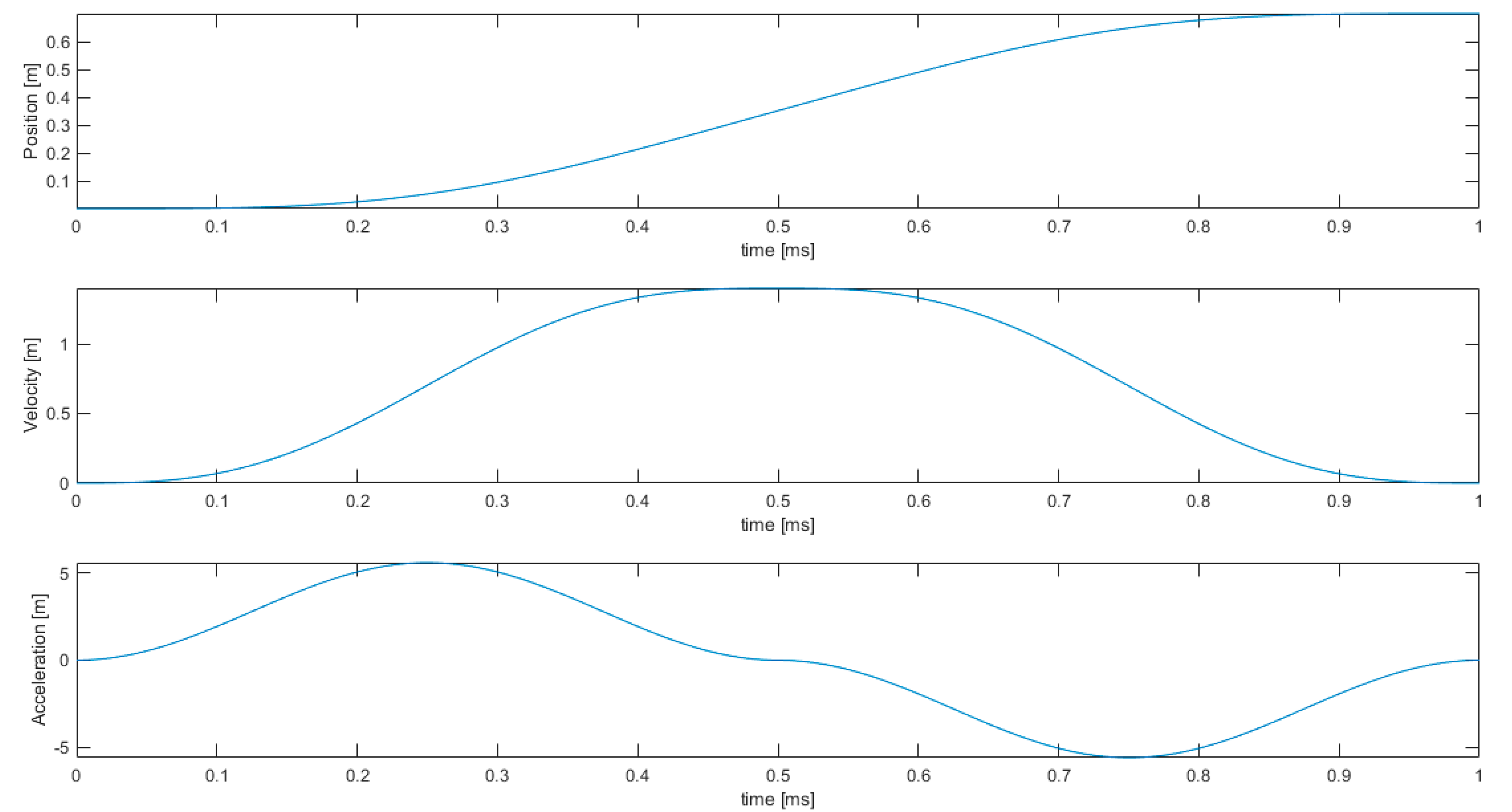
3.2. Simulation Setup
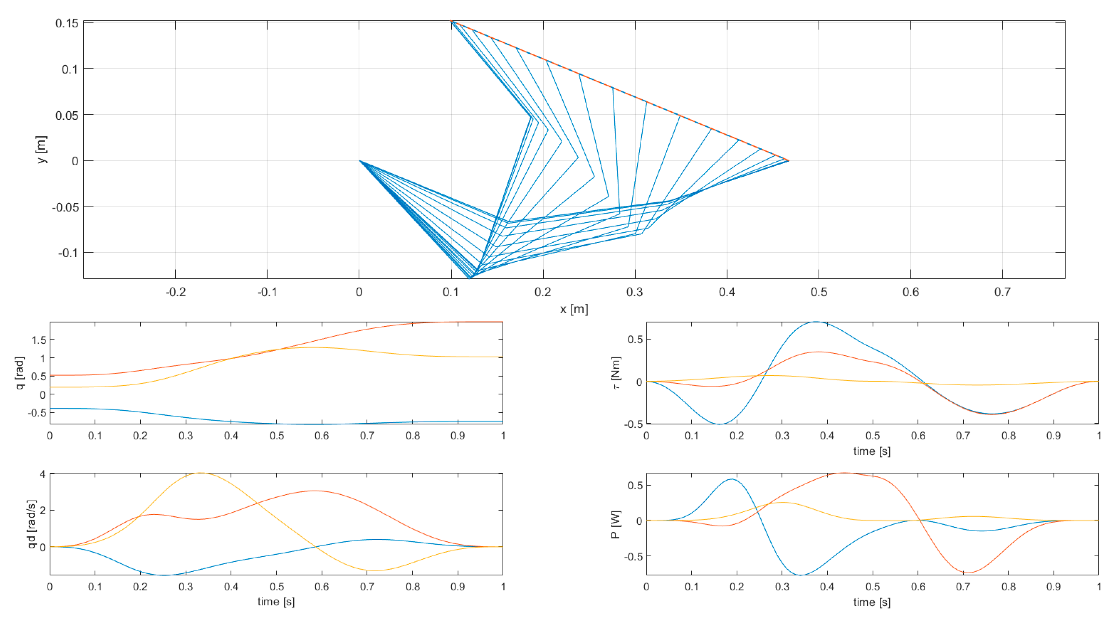
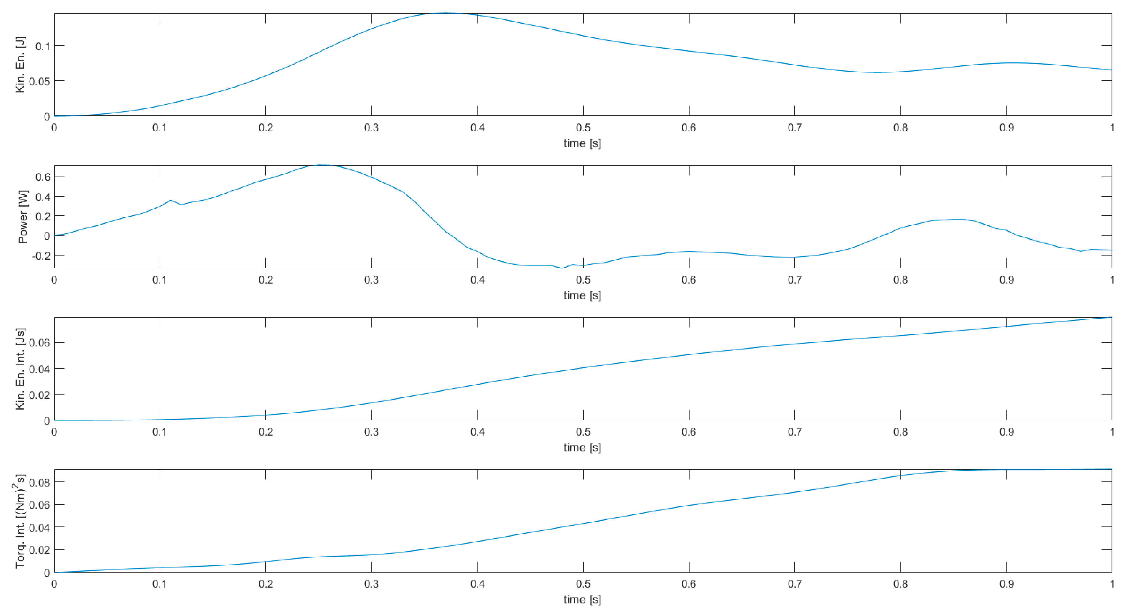
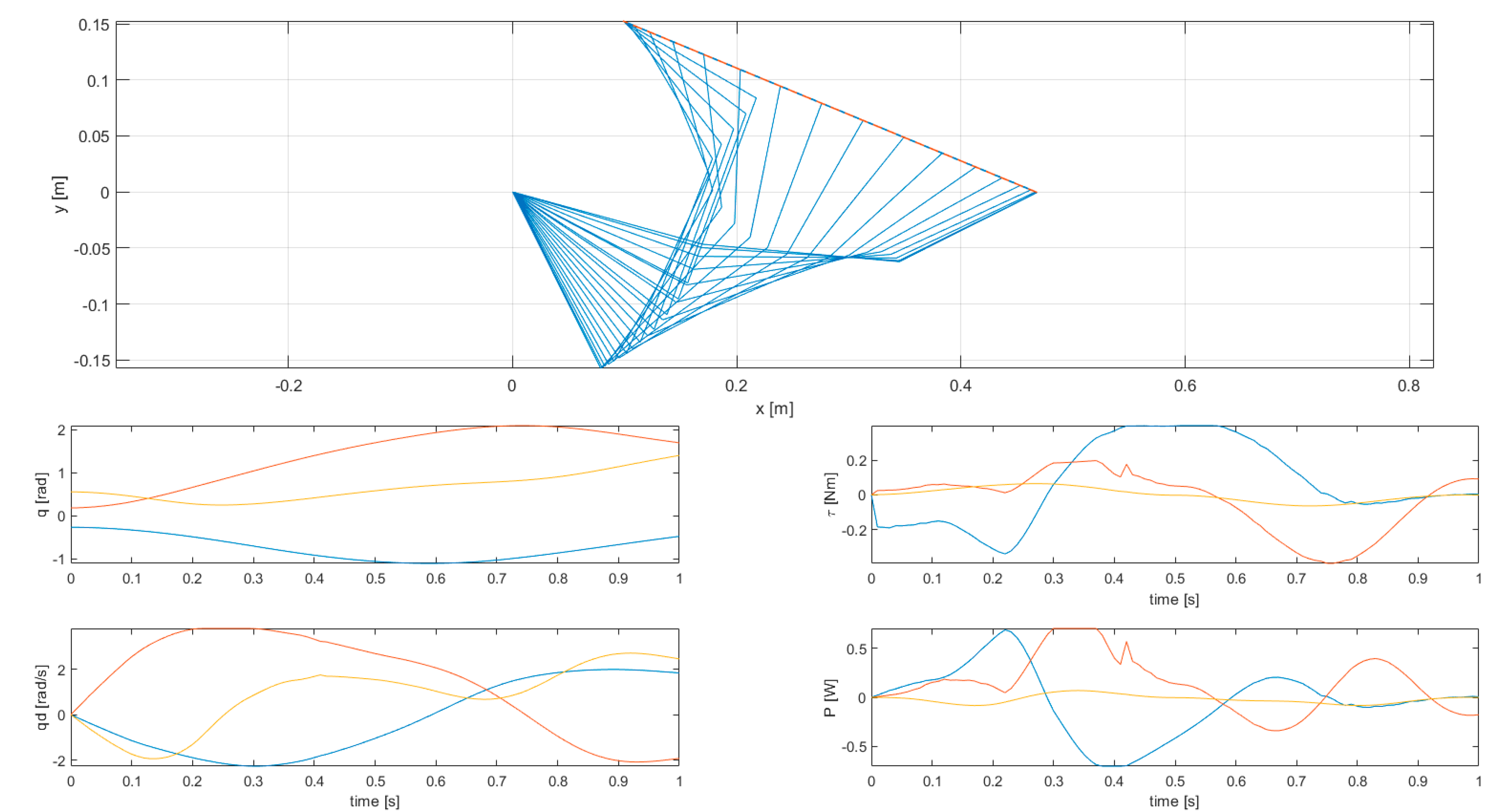
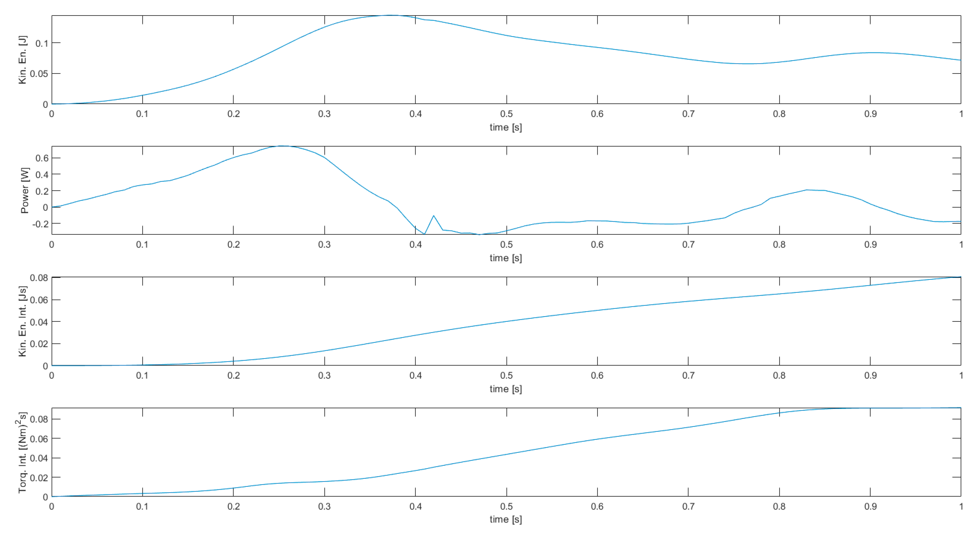
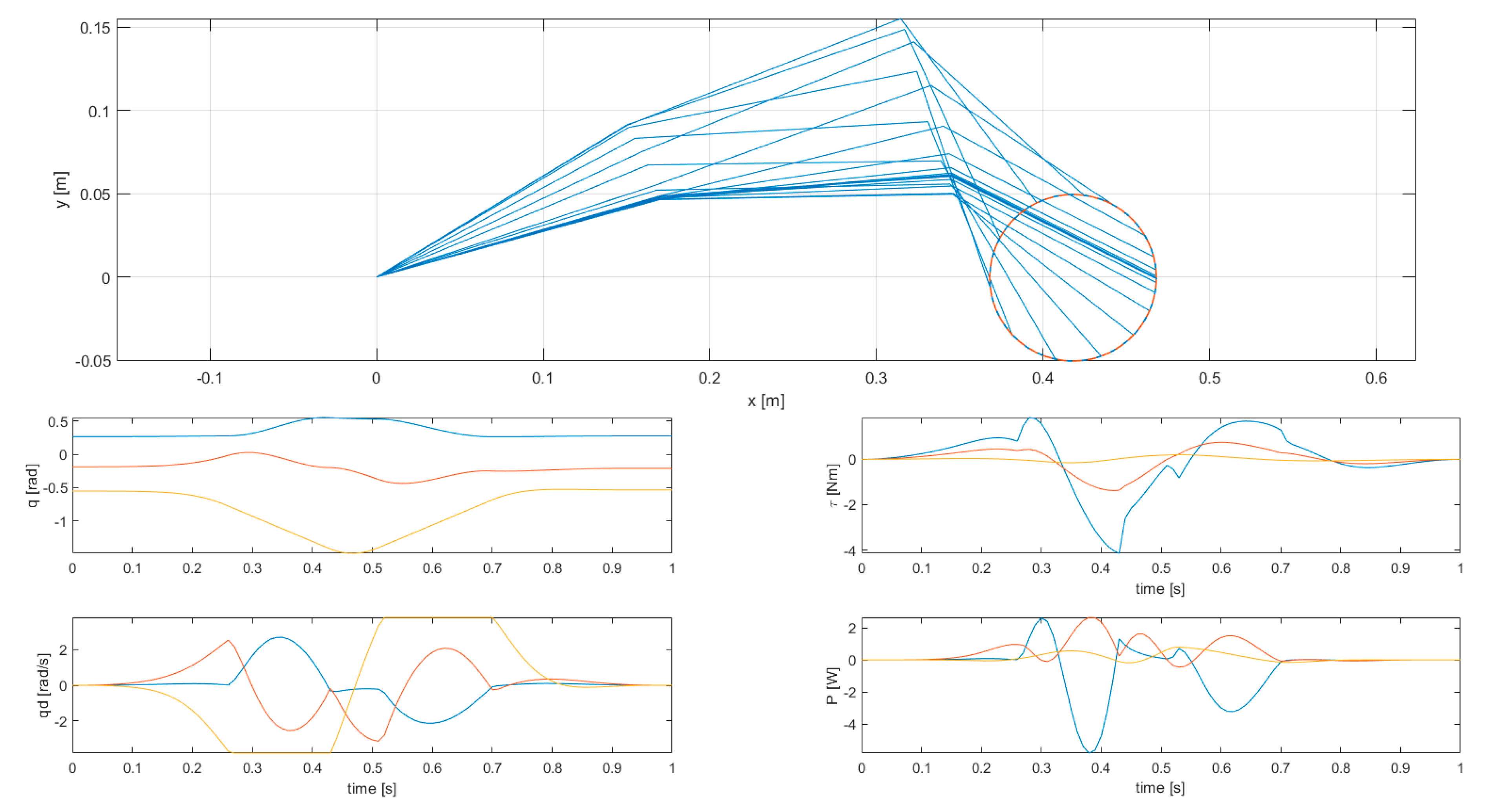
4. Results
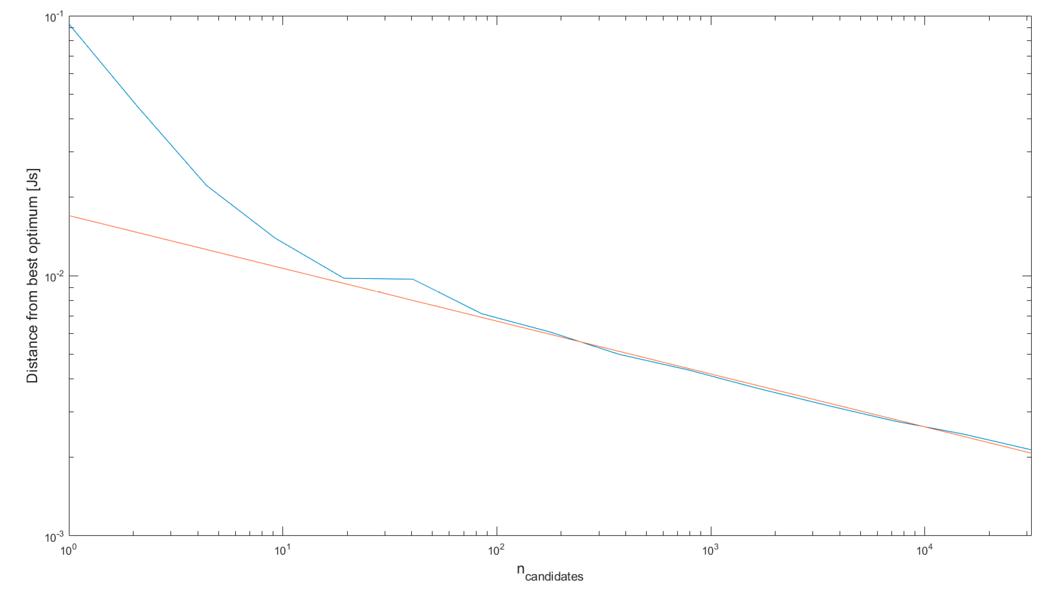
4.1. Validation
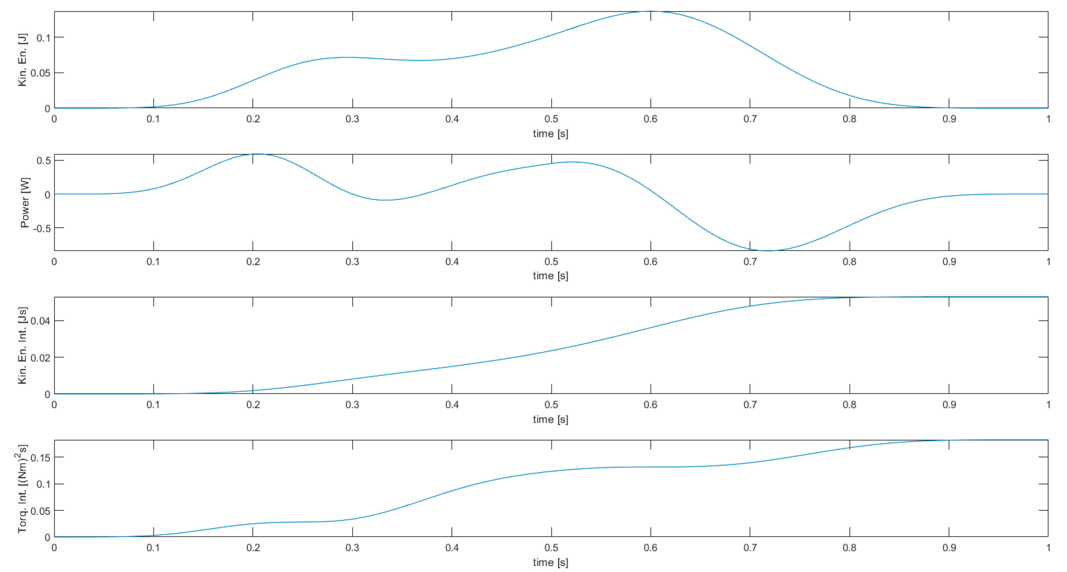
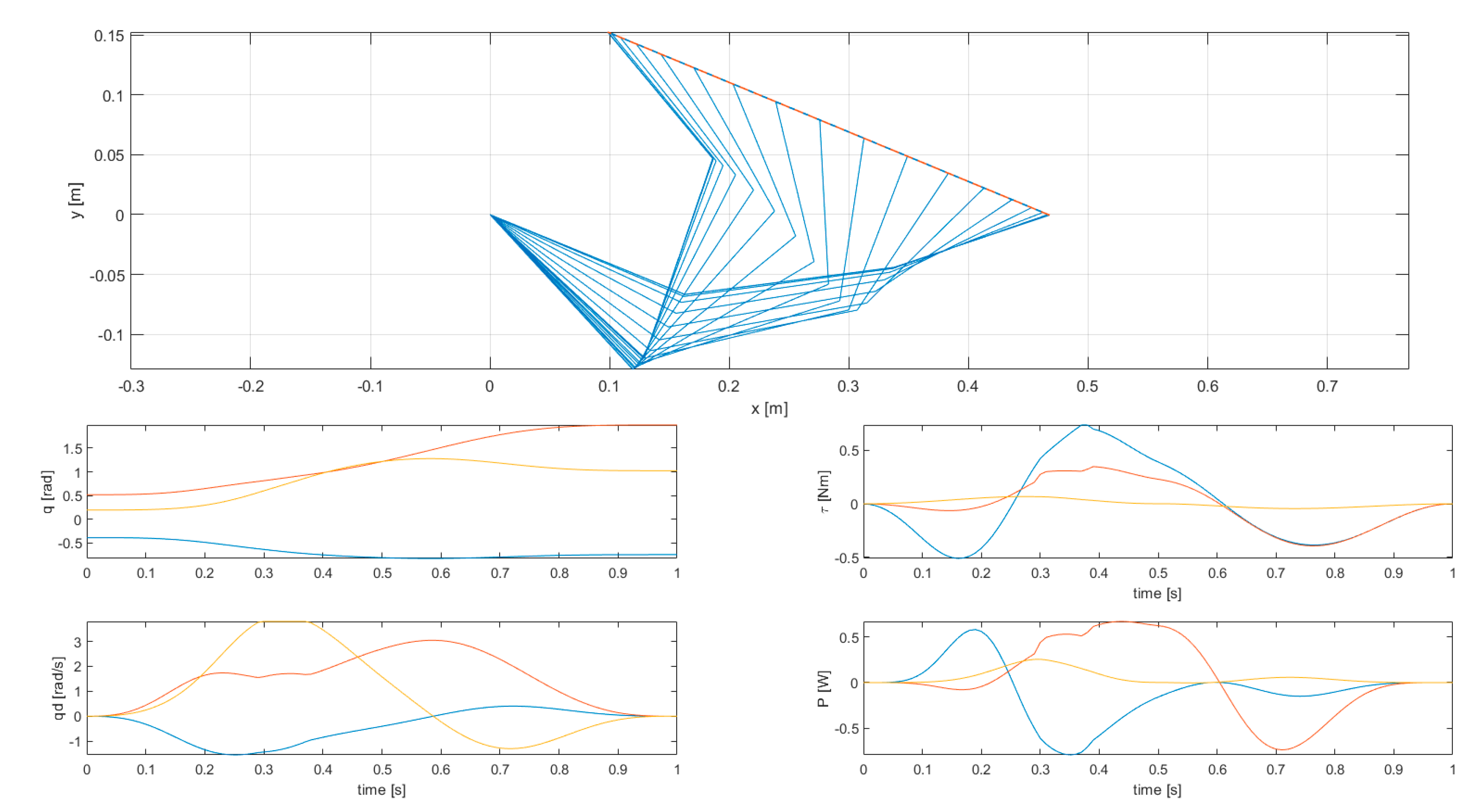
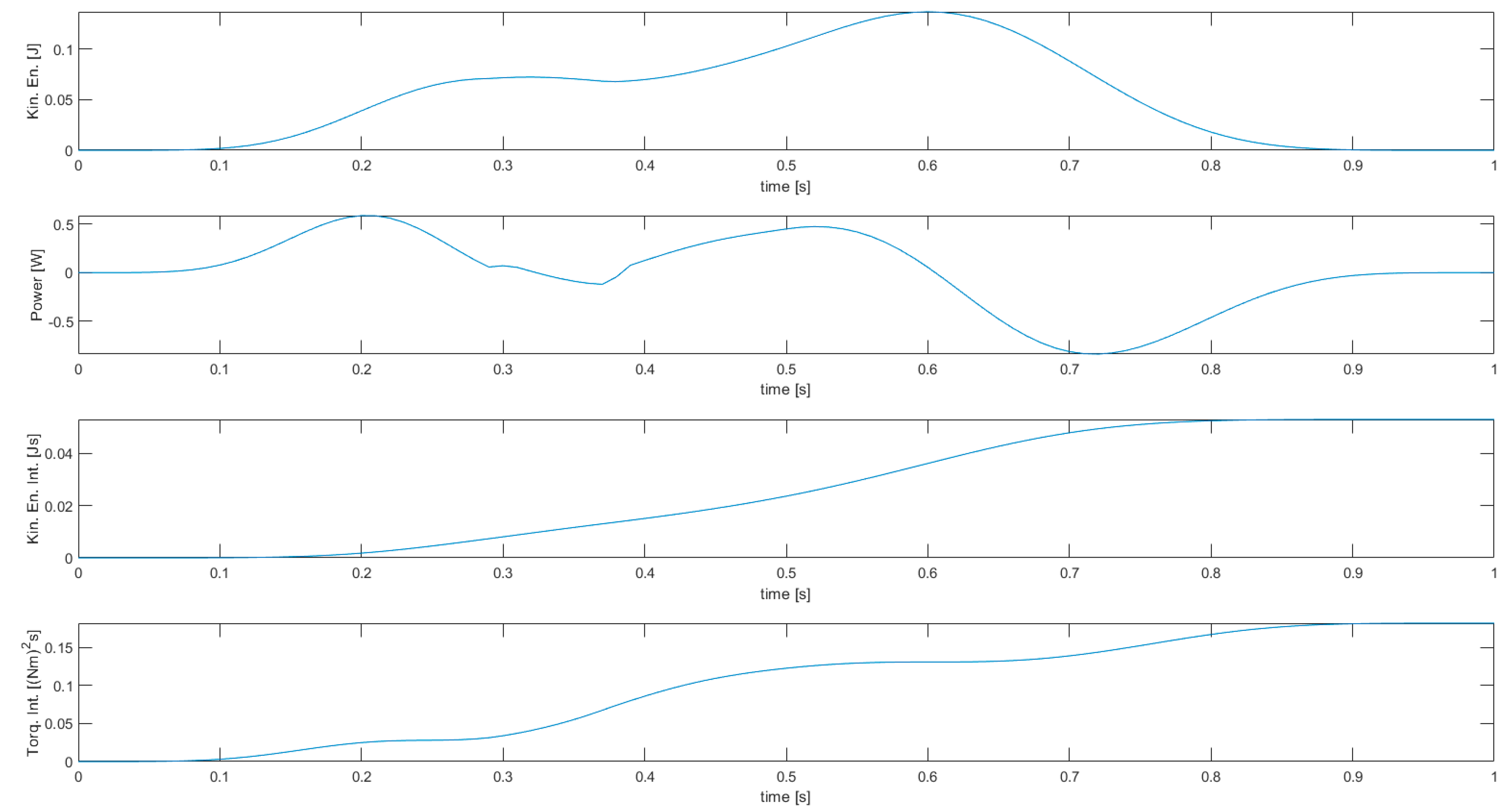
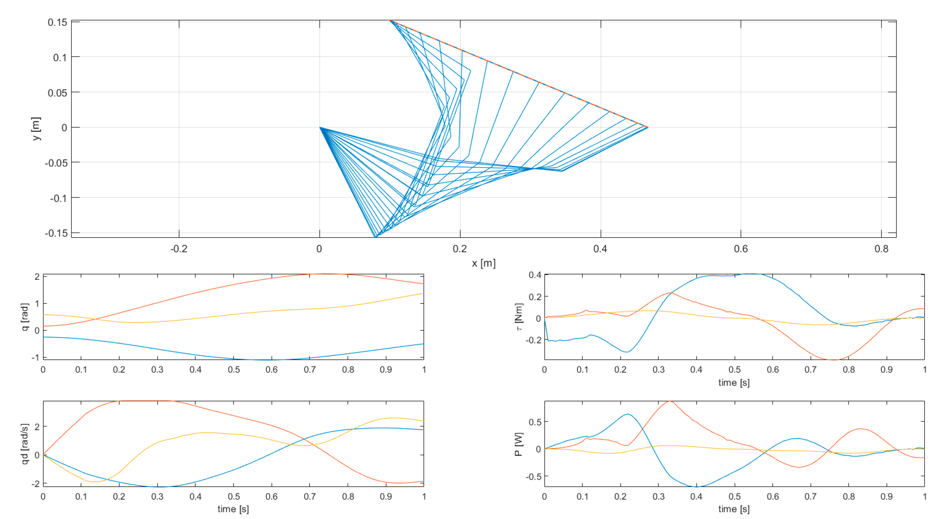
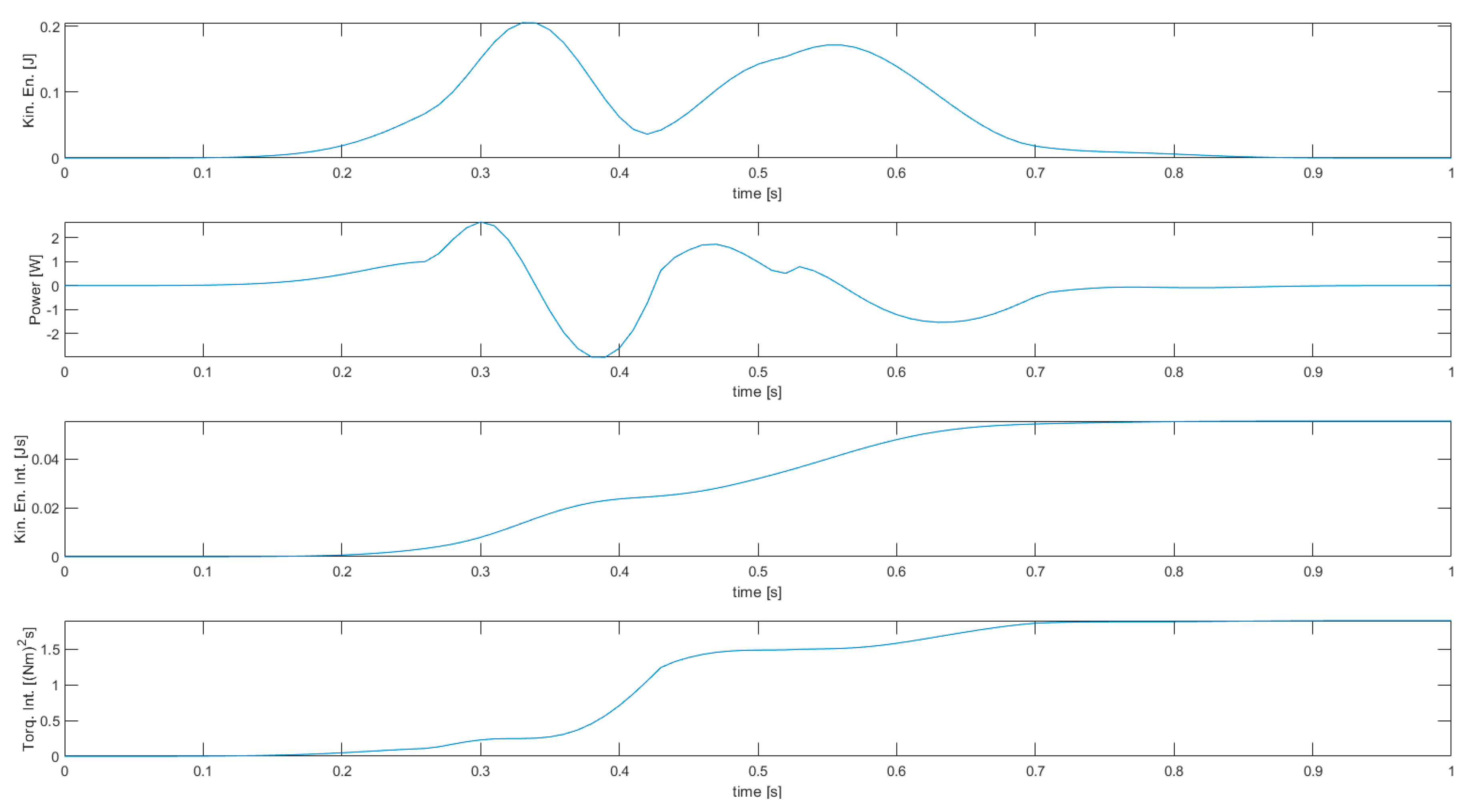
4.2. Simulation Results
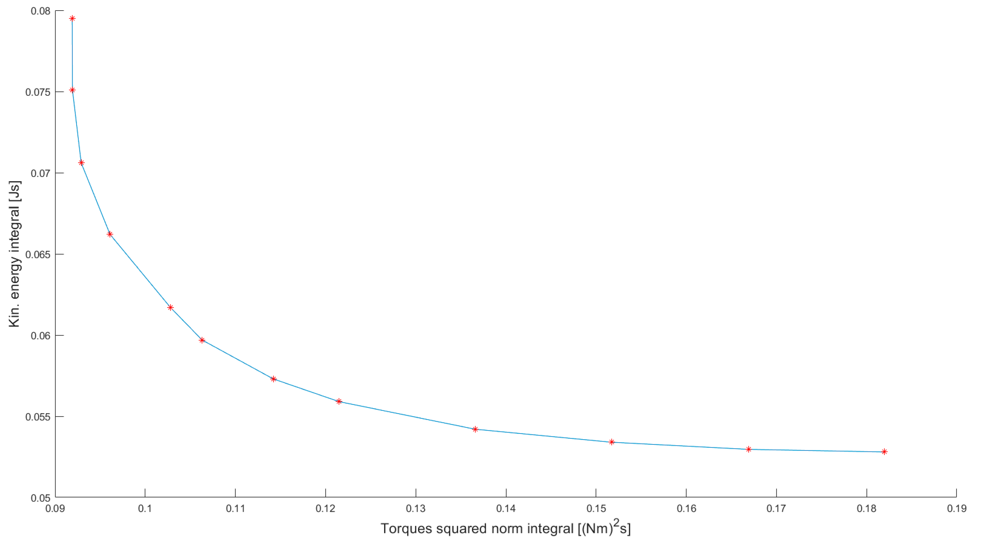
4.3. Multi-Objective Optimization
- 1.
- The feasible solutions resulting in the minima of the two objective functions, (for the minimum of kinetic energy integral) and (for the minimum of torques squared norm integral), are computed separately.
- 2.
- The intervals and are computed.
- 3.
- Each interval is divided in k equally spaced steps and , so that and .
- 4.
- For each a single-objective kinetic energy integral optimization problem is solved with the formulation:
5. Conclusions
Author Contributions
Funding
Conflicts of Interest
References
- Nakamura, Y.; Hanafusa, H.; Yoshikawa, T. Task-Priority Based Redundancy Control of Robot Manipulators. Int. J. Rob. Res. 1987, 6, 32–42. [Google Scholar] [CrossRef]
- Kazerouinian, K.; Wang, Z. Global versus Local Optimization in Redundancy Resolution of Robotic Manipulators. Int. J. Rob. Res. 1988, 7, 3–12. [Google Scholar] [CrossRef]
- Nedungadi, A.; Kazerouinian, K. A local solution with global characteristics for the joint torque optimization of a redundant manipulator. J. Robot. Syst. 1989, 6, 631–654. [Google Scholar] [CrossRef]
- Hirakawa, A. Trajectory planning of redundant manipulators for minimum energy consumption without matrix inversion. In Proceedings of the International Conference on Robotics and Automation, Albuquerque, NM, USA, 25 April 1997; pp. 1–5. [Google Scholar]
- Martin, B.J.; James, E. Minimum-Effort Motions for Open-Chain Manipulators with Task-Dependent End-Effector Constraints. Int. J. Rob. Res. 1999, 18, 213–224. [Google Scholar] [CrossRef]
- Zhou, Z.; Nguyen, C.C. Joint Configuration Conservation and Joint Limit Avoidance of Redundant Manipulators. In Proceedings of the International Conference on Robotics and Automation, Albuquerque, NM, USA, 25 April 1997; pp. 2421–2426. [Google Scholar]
- Zhou, Z.L.; Nguyen, C.C. Globally Optimal Trajectory Planning for Redundant Manipulators using State Space Augmentation Method. J. Intell. Robot. Syst. Theory Appl. 1997, 19, 105–117. [Google Scholar] [CrossRef]
- Nurmi, J.; Mattila, J. Global energy-optimal redundancy resolution of hydraulic manipulators: Experimental results for a forestry manipulator. Energies 2017, 10, 647. [Google Scholar] [CrossRef] [Green Version]
- Lyu, H.; Song, X.; Dai, D.; Li, J.; Li, Z. Time-optimal and energy-efficient trajectory generation for robot manipulator with kinematic constraints. In Proceedings of the 2017 13th IEEE Conference on Automation Science and Engineering (CASE), Xi’an, China, 20–23 August 2017; pp. 503–508. [Google Scholar]
- Ferrentino, E.; Chiacchio, P. A Topological Approach to Globally-Optimal Redundancy Resolution with Dynamic Programming. In ROMANSY 22, Robot Design, Dynamics and Control; Springer International Publishing: Cham, Switzerland, 2019; pp. 77–85. ISBN 978-3-7091-1378-3. [Google Scholar]
- Guigue, A.; Ahmadi, M.; Langlois, R.; Hayes, M.J. Pareto optimality and multiobjective trajectory planning for a 7-DOF redundant manipulator. IEEE Trans. Robot. 2010, 26, 1094–1099. [Google Scholar] [CrossRef]
- Davidor, Y. Genetic Algorithms and Robotics: A Heuristic Strategy for Optimization; World Scientific Publishing Company: Singapore, 1991. [Google Scholar]
- Shintaku, E. Minimum energy trajectory for an underwater manipulator and its simple planning method by using a genetic algorithm. Adv. Robot. 1998, 13, 115–138. [Google Scholar] [CrossRef]
- McAvoy, B.; Sangolola, B.; Szabad, Z. Optimal trajectory generation for redundant planar manipulators. In Proceedings of the 2000 IEEE International Conference on Systems, Man & Cyberbetics, Nashville, TN, USA, 8–11 October 2000; pp. 3241–3246. [Google Scholar]
- Tian, L.; Collins, C. Motion planning for redundant manipulators using a floating point genetic algorithm. J. Intell. Robot. Syst. Theory Appl. 2003, 38, 297–312. [Google Scholar] [CrossRef]
- Baba, N.; Kubota, N. Collision avoidance planning of a robot manipulator by using genetic algorithm—A consideration for the problem in which moving obstacles and/or several robots are included in the workspace. In Proceedings of the First IEEE Conference on Evolutionary Computation, Orlando, FL, USA, 27–29 June 1994; pp. 714–719. [Google Scholar]
- Kazem, B.I.; Mahdi, A.I.; Oudah, A.T. Motion Planning for a Robot Arm by Using Genetic Algorithm. Jordan J. Mech. Ind. Eng. 2008, 2, 131–136. [Google Scholar]
- Ferrentino, E.; Della Cioppa, A.; Marcelli, A.; Chiacchio, P. An Evolutionary Approach to Time-Optimal Control of Robotic Manipulators. J. Intell. Robot. Syst. Theory Appl. 2019, 245–260. [Google Scholar] [CrossRef]
- Stevo, S.; Sekaj, I.; Dekan, M. Optimization of Energy in Robotic arm using Genetic Algorithm. In Proceedings of the 19th World Congress The International Federation of Automatic Control, Cape Town, South Africa, 24–29 August 2014. [Google Scholar]
- Hansen, C.; Kotlarski, J.; Ortmaier, T. Experimental validation of advanced minimum energy robot trajectory optimization. In Proceedings of the 2013 16th International Conference on Advanced Robotics (ICAR), Montevideo, Uruguay, 25–29 November 2013. [Google Scholar] [CrossRef]
- Doan, N.C.N.; Tao, P.Y.; Lin, W. Optimal redundancy resolution for robotic arc welding using modified particle swarm optimization. In Proceedings of the 2016 IEEE International Conference on Advanced Intelligent Mechatronics (AIM), Banff, AB, Canada, 12–15 July 2016; pp. 554–559. [Google Scholar]
- Garg, D.P.; Kumar, M. Optimization techniques applied to multiple manipulators for path planning and torque minimization. Eng. Appl. Artif. Intell. 2002, 15, 241–252. [Google Scholar] [CrossRef] [Green Version]
- Martin, D.P.; Baillieul, J.; Hollerbach, J.M. Resolution of Kinematic Redundancy Using Optimisation Techniques. IEEE Trans. Robot. Autom. 1989, 5, 529–533. [Google Scholar] [CrossRef]
- Pashkevich, A.P.; Dolgui, A.B.; Chumakov, O.A. Multiobjective optimization of robot motion for laser cutting applications. Int. J. Comput. Integr. Manuf. 2004, 17, 171–183. [Google Scholar] [CrossRef]
- Dolgui, A.; Pashkevich, A. Manipulator motion planning for high-speed robotic laser cutting. Int. J. Prod. Res. 2009, 47, 5691–5715. [Google Scholar] [CrossRef] [Green Version]
- Gao, J.; Pashkevich, A.; Caro, S. Optimization of the robot and positioner motion in a redundant fiber placement workcell. Mech. Mach. Theory 2017, 114, 1339–1351. [Google Scholar] [CrossRef]
- Reiter, A.; Muller, A.; Gattringer, H. On Higher Order Inverse Kinematics Methods in Time-Optimal Trajectory Planning for Kinematically Redundant Manipulators. IEEE Trans. Ind. Informat. 2018, 14, 1681–1690. [Google Scholar] [CrossRef]
- Reiter, A.; Gattringer, H.; Müller, A. Redundancy resolution in minimum-time path tracking of robotic manipulators. In Proceedings of the International Conference on Informatics in Control, Automation and Robotics (ICINCO), Lisbon, Portugal, 29–31 July 2016; Volume 2, pp. 61–68. [Google Scholar] [CrossRef] [Green Version]
- Martì, R. Multi-Start Methods. In Handbook of Metaheuristics; Glover, F., Kochenberger, G.A., Eds.; International Series in Operations Research & Management Science; Springer: Boston, MA, USA, 2003; Volume 57. [Google Scholar]
- Solis, F.J.; Wets, R.J.-B. Minimization by Random Search Techniques. Math. Oper. Res. 1981, 6, 19–30. [Google Scholar] [CrossRef]
- Nocedal, J.; Wright, S. Numerical Optimization; Springer Science & Business Media: Berlin/Heidelberg, Germany, 2006. [Google Scholar]
- Liegeois, A. Automatic Supervisory Control of the Configuration and Behavior of Multibody Mechanisms. IEEE Trans. Syst. Man Cybern. 1977, 7, 868–871. [Google Scholar]
- Beckman, R.J.; Conover, W.J.; McKay, M.D. A comparison of three methods for selecting values of input variables in the analysis of output from a computer code. Technometrics 1979, 21, 239–245. [Google Scholar]
- Cocuzza, S.; Pretto, I.; Debei, S. Least-Squares-Based Reaction Control of Space Manipulators. J. Guid. Control. Dyn. 2012, 35, 976–986. [Google Scholar] [CrossRef]
- Cocuzza, S.; Pretto, I.; Debei, S. Novel reaction control techniques for redundant space manipulators: Theory and simulated microgravity tests. Acta Astronaut. 2011, 68, 1712–1721. [Google Scholar] [CrossRef]
- Cocuzza, S.; Tringali, A.; Yan, X.-T. Energy-efficient motion of a space manipulator. In Proceedings of the International Astronautical Congress, IAC, Guadalajara, Mexico, 26–30 September 2016. [Google Scholar]
- Tringali, A.; Cocuzza, S. Predictive control of a space manipulator through error and kinetic energy expectation. In Proceedings of the International Astronautical Congress, Bremen, Germany, 1–5 October 2018. [Google Scholar]
- Ferrentino, E.; Chiacchio, P. On the Optimal Resolution of Inverse Kinematics for Redundant Manipulators Using a Topological Analysis. J. Mech. Robot. 2020, 12, 1–14. [Google Scholar] [CrossRef]
- Das, I.; Dennis, J.E. A closer look at drawbacks of minimizing weighted sums of objectives for Pareto set generation in multicriteria optimization problems. Struct. Optim. 1997, 14, 63–69. [Google Scholar] [CrossRef] [Green Version]
- Chircop, K.; Zammit-Mangion, D. On Epsilon-Constraint Based Methods for the Generation of Pareto Frontiers. J. Mech. Eng. Autom. 2013, 3, 279–289. [Google Scholar]


| Link # | Mass (kg) | Length (m) | Moment of Inertia (Barycentric) (kgm2) | Center of Gravity (m) |
|---|---|---|---|---|
| 1 | 0.615 | 0.176 | 0.001811 | 0.0950 |
| 2 | 0.615 | 0.176 | 0.003173 | 0.0717 |
| 3 | 0.307 | 0.1375 | 0.002103 | 0.0526 |
| Constraint | Value |
|---|---|
| Joint displacement | 90 deg on 1st joint, 120 deg on 2nd and 3rd joint |
| Joint velocity | 3.8 rad/s |
| Joint torque | 0.4 Nm |
| Joint power | 0.7 W |
| Simulation nr. | Shape | Control Cost | Constraints |
|---|---|---|---|
| 1 | Rectilinear | Kinetic energy | Unconstrained (validation) |
| 2 | Rectilinear | Kinetic energy | Joint displacement, velocity |
| 3 | Rectilinear | Torques norm | Joint displacement, velocity |
| 4 | Rectilinear | Torques norm | Joint displacement, velocity, torque, power |
| 5 | Circular | Kinetic energy | Joint displacement, velocity, cyclic motion |
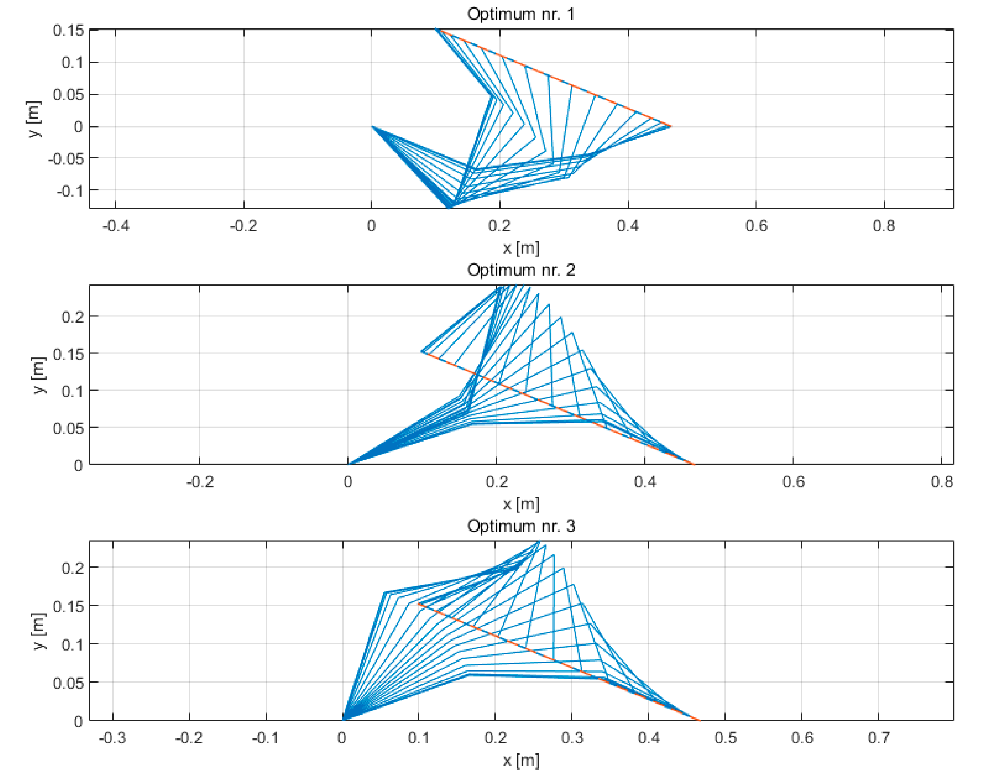
| Optimum nr. | Nedungadi—Kinetic Energy Integral (Js) | Interpolation-Based Global Kinematic Planner—Kinetic Energy Integral (Js) | Mean Absolute Difference of Joint Displacements (rad) |
|---|---|---|---|
| 1 | 0.0532 | 0.0528 | 8.5 × 10⁻³ |
| 2 | 0.0567 | 0.0563 | 2.2 × 10⁻² |
| 3 | 0.0673 | 0.0671 | 3.8 × 10⁻³ |
| Simulation nr. | Cost Function | Kinetic Energy Integral (Js) | Torques Squared Norm Integral ((Nm)2s) | Computational Time (s) |
|---|---|---|---|---|
| 1 | Kin. Energy | 0.0528 | 0.1827 | 290 |
| 2 | Kin. Energy | 0.0528 | 0.1820 | 218 |
| 3 | Torques norm | 0.0795 | 0.0912 | 276 |
| 4 | Torques norm | 0.0808 | 0.0916 | 160 |
| Simulation nr. | Cost Function | Kinetic Energy Integral (Js) | Torques Squared Norm Integral ((Nm)2s) | Computational Time (s) |
|---|---|---|---|---|
| 5 | Kin. Energy | 0.0554 | 1.898 | 282 |
© 2020 by the authors. Licensee MDPI, Basel, Switzerland. This article is an open access article distributed under the terms and conditions of the Creative Commons Attribution (CC BY) license (http://creativecommons.org/licenses/by/4.0/).
Share and Cite
Tringali, A.; Cocuzza, S. Globally Optimal Inverse Kinematics Method for a Redundant Robot Manipulator with Linear and Nonlinear Constraints. Robotics 2020, 9, 61. https://doi.org/10.3390/robotics9030061
Tringali A, Cocuzza S. Globally Optimal Inverse Kinematics Method for a Redundant Robot Manipulator with Linear and Nonlinear Constraints. Robotics. 2020; 9(3):61. https://doi.org/10.3390/robotics9030061
Chicago/Turabian StyleTringali, Alessandro, and Silvio Cocuzza. 2020. "Globally Optimal Inverse Kinematics Method for a Redundant Robot Manipulator with Linear and Nonlinear Constraints" Robotics 9, no. 3: 61. https://doi.org/10.3390/robotics9030061