Review

A Review of Trajectory Prediction Methods for the Vulnerable Road User

by
Erik Schuetz
* and
Fabian B. Flohr
Intelligent Vehicles Lab, Munich University of Applied Sciences, Lothstr. 34, 80335 Munich, Germany
*
Author to whom correspondence should be addressed.
Robotics 2024, 13(1), 1; https://doi.org/10.3390/robotics13010001
Submission received: 30 October 2023 / Revised: 11 December 2023 / Accepted: 16 December 2023 / Published: 19 December 2023
(This article belongs to the Special Issue Motion Trajectory Prediction for Mobile Robots)

Abstract

:
Predicting the trajectory of other road users, especially vulnerable road users (VRUs), is an important aspect of safety and planning efficiency for autonomous vehicles. With recent advances in Deep-Learning-based approaches in this field, physics- and classical Machine-Learning-based methods cannot exhibit competitive results compared to the former. Hence, this paper provides an extensive review of recent Deep-Learning-based methods in trajectory prediction for VRUs and autonomous driving in general. We review the state and context representations and architectural insights of selected methods, divided into categories according to their primary prediction scheme. Additionally, we summarize reported results on popular datasets for all methods presented in this review. The results show that conditional variational autoencoders achieve the best overall results on both pedestrian and autonomous driving datasets. Finally, we outline possible future research directions for the field of trajectory prediction in autonomous driving.

1. Introduction

Autonomous driving is presently at the heart of the automotive industry, attracting numerous research institutes globally. High-profile companies such as Zoox, Cruise, and Waymo are making impressive strides in the latest iterations of their autonomous taxis [1,2,3]. This significant progress has drawn the public’s attention to the field.
A crucial aspect of autonomous vehicles is the capacity to anticipate the future behaviors of other road users, particularly in urban settings. In these environments, the traffic often includes vulnerable road users (VRUs), and predicting their movements is inherently more challenging than predicting the movements of vehicles. This is due to a number of reasons. Firstly, pedestrians are not bound by non-holonomic constraints and can thus change their movement with more degrees of freedom than vehicles [4]. Secondly, guessing the ulterior goals of VRUs is more difficult in traffic scenarios as they do not have to stay in a lane like vehicles. Thirdly, the margin of error is much narrower as collisions stemming from erroneous predictions have a higher probability of leading to the loss of life. A better understanding of other road users’ behaviors would assist in planning the autonomous vehicle’s trajectory, reducing the need for unexpected maneuvers that could necessitate a complete trajectory replanning or even result in a collision. This also involves understanding how road users interact with each other to plan their own trajectories. Figure 1 schematically shows the influences on the possible trajectories of road users in a scene.
The importance of accurate trajectory prediction in autonomous driving has attracted extensive research interest, as evidenced by the multitude of studies presented at recent prestigious conferences such as CVPR 2023 [5] and ICCV 2023 [6]. Several reviews have focused on the topic of Deep Learning methods for trajectory prediction [7,8]. Huang et al. [9] not only included Deep Learning methods but also physics-based, classic Machine-Learning-based, Deep-Learning-based, and Reinforcement-Learning-based methods. Unfortunately, these surveys ignored the important aspect of pedestrian motion prediction in autonomous driving. The works by Ridel et al. [10] and Rudenko et al. [11] reviewed VRU (pedestrian) trajectory prediction methods but failed to put them into context with methods developed on autonomous driving datasets for the prediction of all traffic participants. Huang et al. [9] showed in their survey that physics-based and classical Machine-Learning-based methods are inferior to deep neural networks with respect to prediction quality. Additionally, the surveys cited above fell short of capturing recent advancements made with deep neural networks in the field of trajectory prediction. Therefore, we introduce our comprehensive review of Deep-Learning-based trajectory prediction techniques within the context of autonomous driving, focusing on the VRU, with our contributions being three-fold:
  • We summarize and synthesize recent Deep Learning strategies for enhancing trajectory prediction in autonomous driving, focusing on VRU safety. To the best of our knowledge, no comparable studies have delved into recent Deep Learning methods to this extent.
  • We scrutinize various interaction models, revealing critical input features driving the success of prevalent prediction methods, and give an in-depth summary of possible output modes.
  • We provide extensive insight into the efficacy of methods on various datasets, conduct a rigorous analysis of the results, and identify promising further research directions.
The paper is organized as follows: In Section 2, we briefly introduce the problem description of trajectory prediction (Section 2.1) and explain our classification taxonomy together with a short explanation of how the methods were collected (Section 2.2). Section 3 first details possible input features, then reviews the scene representations and interaction modeling schemes employed by the subsequently introduced methods. Lastly, this section also scrutinizes the trajectory output strategies employed. Section 4 introduces the selected methods clustered by their prediction category. Section 5 begins with a brief introduction to commonly used datasets and metrics for trajectory prediction, then presents the reported results of the introduced methods. Lastly, this section discusses the presented results and offers potential future research directions. In the last chapter, we summarize the paper and offer a short conclusion.

2. Fundamentals and Taxonomy

2.1. Problem Formulation

Consider a traffic scene containing N agents of any class, where each agent i at timestep t can be described by a state denoted as x i t . The goal of this problem is to predict sequences of positions, i.e., trajectories; thus, one can adapt the problem formulation for sequence generation tasks from Graves [12] to this application. With this adaptation, the problem of trajectory prediction in autonomous driving can be formulated as the prediction of a sequence Y i of k future positions denoted as Y i = { y i T + 1 , y i T + 2 , , y i T + k } for an agent i in the scene from an input sequence of T observed states denoted as X i = { x i 1 , x i 2 , , x i T } of an agent i, where y i T + 1 is the future position of agent i at timestep T + 1 . An observed state can be any property of agent i at timestep t, which also includes latent features or a direct sensor input. Possible properties or states, e.g., position, velocity, or heading, are introduced in Section 3.1. In an autonomous driving setting, incorporating the movement of the autonomous vehicle in these transformations and also in the input positions X is also required. With the above-derived definitions, we can formulate a trajectory prediction equation connecting the input X i with the output Y i using an unknown function f for a single agent i (adapted from Huang et al. [9]):
Y i = f X i .
As the dimensionality and complexity of f are unknown, constraining the expressivity of the predictor through the manual engineering of features or model choice (e.g., physics-based models [9]) could lead to reduced prediction performance. Using a data-driven approach with as few manual influences as possible allows the model to learn the underlying complexities of the problem through examples. Since Multilayer Perceptrons, and thus deep neural networks, can be considered to be general function approximations, and due to the success of Deep Learning methods in other domains such as computer vision [13], we can transfer the problem formulation to a Deep Learning context with a Deep Learning model M for N agents as [14]
{ Y } i = 1 N = M { X } i = 1 N ,
where M approximates the unknown function f connecting the input and output features of the trajectory prediction problem. However, many Deep Learning methods do not output Y directly but rather model the underlying probability distribution p ( Y | X ) . This distribution can be multimodal to model different movement choices of agents, like taking a left or a right turn, which is clarified in Figure 2. Sampling Y i from the modeled p ( Y i | X i ) given an input sample X i allows one to extract trajectories from the modeled distribution.
Additionally, one can differentiate between marginal and joint predictions for agents. Marginal predictions are predictions for a single agent i without considering other agents in the scene, resulting in the probability distribution given above. Joint predictions are predictions for an agent i considering other agents j i in the scene, yielding the probability distribution q Y i | X i , X j j = 1 N . The latter is more challenging as it requires modeling the interactions between agents and making scene-consistent predictions without collisions. This can be extended to pairwise, groupwise, or scene-wide joint predictions [15,16,17]. Figure 3 illustrates the difference between marginal and joint predictions for a scene with two independent agents. While marginal predictions are carried out separately for every agent, assuming no other agents in the scene, joint predictions consider possible interactions between agents and provide, in this example, pairwise predictions without predicted collisions.

2.2. Classification Taxonomy and Method Selection

This section will give a short overview of the classification taxonomy used in this survey. For trajectory prediction methods based on models beyond Deep Learning, we refer the interested reader to the excellent survey on trajectory prediction methods for autonomous driving by Huang et al. [9].
The methods introduced in this review were classified according to the considerations of their primary prediction scheme. Some methods could arguably be assigned to multiple classes but were assigned to one for the sake of this review. The proposed categories are diffusion-based, anchor-based, generative adversarial network (GAN)-based, conditional variational autoencoder (CVAE)-based, recurrent neural network (RNN)-based, Transformer- and attention-based, convolutional neural network (CNN)-based, temporal convolutional network (TCN)-based, graph neural network (GNN)-based, and set-based methods. Methods that did not fit any other category were assigned to “Other”. This also included some end-to-end methods that directly predict the movement of LiDAR points. As RNNs and graph-based approaches were also present in some of the other categories at interim positions, methods were only assigned to these two categories if they mainly relied on RNNs or GNNs for their predictions.
This review considers important methods published between the years 2021 and 2023 using Deep-Learning-based approaches for the problem of trajectory prediction in the domains of autonomous driving and pedestrian prediction. However, some exceptions are made for older, interesting, and still relevant publications that have been cited throughout recent works. The methods were collected by scanning the benchmark leaderboards of commonly used datasets (see Section 5.1), reviewing publications of prestigious conferences like CVPR and ICCV, and conducting searches within the year constraints given above for the keywords “trajectory prediction”, “pedestrian trajectory prediction”, and “motion forecasting” on Google Scholar. The methods were chosen based on their architectural insights and their reported trajectory prediction performance. Table 1 gives an overview of all methods reviewed in this paper.

3. State and Context Representation

This chapter will first give an overview of how to approach the problem of Deep-Learning-based trajectory prediction by introducing possible input features, ways to represent a scene and model interactions, and commonly used ways to output trajectory predictions.

3.1. Possible Input Features

Commonly used input features can be categorized into agent-specific and environmental input features. While agent-specific features describe some part of the agent’s state, environmental features describe the scene’s static surroundings (here, traffic lights and their states are considered static).
Among the agent-specific input features, the 2D position of each agent, viewed from a bird’s eye view (BEV) perspective, is the most prevalent feature employed by almost all trajectory prediction methods [16,20,27,30,37,42,54,61,67,69,72,84,91,96,100,101,102,103,104,105]. This method uses the 2D position with global or local scene coordinates depending on its application. For instance, Gu et al. [29] used a local coordinate scheme, where the trajectory and surroundings of the agent of interest were transformed into a local coordinate system with the agent at the origin. This process was repeated for every agent in the scene. Encoding the positions with a global coordinate system is typically used in static scenes, such as the surveillance scenes in the ETH/UCY datasets [106,107] or drone scenes in the Stanford Drone Dataset (SDD) [108], given the sensor’s origin never changes. Using a global frame of reference potentially leads to more efficient computations as agent features have to be computed once and can be reused for multiple agents of interest. However, the downside of this approach is a potential loss of pose invariance [17]. Local frames of reference require transforming agent positions into every agent’s frame of reference, which benefits the pose invariance of the model but scales linearly with the number of agents [17]. Zhang et al. [58] employed a third approach to parse the 2D positions, supplying the method with the trajectory of each agent as a sequence of relative positions, or position changes.
Apart from the agent’s position, some methods also utilize the heading angle ψ as input. Chen et al. [16] used the heading angle in the form of a feature vector containing cos ( ψ ) and sin ( ψ ) to avoid confusion in the network when distinguishing between 2 π and 2 π , although they represent the same angle. Another frequently used feature is the agent’s velocity. Rowe et al. [85] incorporated the velocity as v R 2 , alongside the agent’s position p R 2 and the agent’s heading angle ψ , in their input feature vector x = p , v , ψ . Explicitly adding features like the heading angle and velocity, even though they were implicitly present in the sequence of positions, gave the model additional focus on these features. Furthermore, these features could be used to further describe and construct interactions between agents [16].
Another agent-specific feature recently incorporated into some methods is the pose of vulnerable road users. The premise behind using the pose is that it can provide insight into the intentions of vulnerable road users (for instance, cyclists’ gestures indicating a turn). Su et al. [45] employed a pose estimator to extract the positions of 17 joints as heatmaps for further use in the model [109]. Kress et al. [105] followed a different approach and provided the explicit positions of 13 joints of a VRU as input for their method.
The accurate prediction of possible future trajectories requires the consideration of static objects in the agent’s surroundings through environmental features. To this end, many methods add high-definition (HD) maps to agent-specific features to support their predictions [29,57,60,68,69,73,91]. HD maps are centimeter-accurate digital representations of physical environments, integrating detailed geospatial information and infrastructure details, such as lane information [110]. The use of these maps is contingent upon their availability in the relevant dataset or location. The current state-of-the-art method for using and encoding HD maps in a trajectory prediction approach is VectorNet [110], which encodes the features of an HD map as polylines using a vector-based graph representation of the scene. This environmental graph representation can be fused with the agents’ features to predict trajectories that align with scene-specific physical constraints. As HD maps are expensive and require regular updates due to environmental changes (e.g., construction sites), alternatives for incorporating static environmental features are sought. Schmidt et al. [111] showed that using navigational maps instead of HD maps by training a method with locally available HD maps and navigational maps via a teacher–student scheme is a viable alternative. In datasets like ETH/UCY, which do not offer maps but only images of the surroundings, methods integrate scene information into their trajectory predictions by encoding environment images using a convolutional neural network (CNN)-based backbone [16,26,28,39,79,96]. Incorporating environmental features (map information) improves the prediction performance as the models are able to learn traversable areas of the agents’ surroundings [110].
Several studies, such as those by Peri et al. [99], Wang et al. [95], Wang et al. [77], and Casas et al. [101], bypassed explicit object and environmental features as introduced above and used raw sensor data (in this case, LiDAR point clouds) as input for their prediction methods. This input format necessitated changes to the prediction methodology; for example, Peri et al. [99] predicted future positions as detection classes, while Wang et al. [95] predicted the motion of each point in the point cloud in voxelized form. A special property of this approach was that a reduced number of human-engineered features were used, which required the model to learn important features from the sensor inputs by itself.

3.2. Scene Representation and Interaction Modeling

Scene representation refers to the method used to depict the configuration of agents in a scene, while interaction modeling pertains to the techniques used to capture the relationships between agents and between agents and their environment.
Many trajectory prediction methods utilize a simple scene representation strategy where the 2D position of agents is used without additional processing [20,26,69,74,102]. However, increasingly, researchers are exploring the use of graph-based scene representations. In these models, agents are represented as nodes in the scene graph, with features encoded as per the discussion in Section 3.1 and the agent’s class [51]. Edges between nodes are used to represent interactions between agents [57], and the inclusion of HD map data enables the modeling of interactions between agents and their environment [85].
For instance, Rowe et al. [85] utilized LaneGCN [112] to merge heterogeneous data from agents and HD maps, allowing for the incorporation of interactions into a common feature space. Similarly, Wang et al. [68] generated separate subgraphs for agents and infrastructure using VectorNet [110]. The nodes of the subgraphs were encoded using fully connected graph neural networks. They then modeled interactions between agents and infrastructure elements using a multi-layer cross-attention network [113]. Gu et al. [29] followed this approach closely but directly used VectorNet’s subgraph and global graph modules to model all interactions. Mo et al. [57] took a different approach by encoding interactions between agents, the agents’ historical states, and the map features separately without explicitly modeling interactions between agents and infrastructure elements. Their system represented the scene as a directed edge-featured heterogeneous graph and used an enhanced graph attention network to extract agent–agent interaction features. Infrastructure interactions were implicitly modeled by supplying all three feature types to the prediction module. Salzmann et al. [51] encoded agent–agent interactions by encoding connecting edges with type-specific LSTMs and aggregating them using an additive attention module. Infrastructure interactions were considered by applying a CNN to the agent-centered area of the HD map and then concatenating the extracted features with the features of each agent node. Chen et al. [16], Xu et al. [87], and Zhou et al. [34] used a group-wise interaction scheme. While Chen et al. [16] only established edges between nodes within a group based on future distances between agents, Xu et al. [87] and Zhou et al. [34] also allowed for intergroup interactions. Zhou et al. [34] further extended this idea by modeling three different interactions: between pedestrians across groups, between pedestrians within one group, and between groups.
Graph-based representations that do not utilize HD maps implicitly model agent–infrastructure interactions by encoding an image of the surroundings or a local map using CNN-based feature extractors [16,39] or not modeling these interactions. Li et al. [72] presented a different approach, where each node in the graph-based scene representation was a local area of the scene, and the edges represented the spatial relationship between these areas. They used a graph-based spatial Transformer network to extract features from these local areas and model pedestrian interactions.
Two methods, one proposed by Mangalam et al. [28] and the other by Lee et al. [42], represented the scene as a heatmap overlayed on the RGB image of the scene, where each channel of the heatmap corresponded to one timestep. This approach simplified the fusion of trajectory and scene information.
Guo et al. [96] offered a unique solution using a directional pooling grid for each agent of interest. Each cell in the grid reflected the relative velocity between the agent of interest and the agent in that cell. This method comprehensively represented the scene and modeled the interactions between the agents using relative velocities and positions. Kamenev et al. [54] used a similar representation featuring two ego-vehicle-centered maps. One map was an occupancy map that rendered other vehicles as rectangles in a bird’s eye view that contained the corresponding velocity vector for each pixel belonging to a vehicle. They did not explicitly model any interactions.
Several other non-graph-based interaction modeling techniques exist. Gupta et al. [37] introduced social pooling, where the module concatenated the relative positions between the agent of interest and other agents in the scene. It then processed this through an MLP and a max pooling layer. This method allowed the network to convey interaction information between every agent in the scene. Mangalam et al. [31] also applied a form of social pooling, but instead of using explicit features, they used the encoded representations of trajectories and waypoints for every agent. They fused the representations for every agent using a non-local attention mechanism, which allowed the network to learn the social pooling mechanism.
Several methods, such as those proposed by Huang et al. [69], Sun and Sun [76], Xie et al. [43], Zhou et al. [73], Wang et al. [60], and Ngiam et al. [17], employ attention mechanisms, specifically transformer layers, to encode the interactions between agents. Chen et al. [61] used cross-attention between the encoded agent trajectory and the intentions of surrounding agents to perform conditional predictions, effectively modeling interactions between agents. Sun et al. [15] and Li et al. [27] also utilized conditional predictions to model interactions. Sun et al. [15] classified agents as influencers and influenced agents and then conditioned the influenced agent’s prediction on the influencer’s marginal prediction. Li et al. [27] used a goal-conditioned prediction scheme where the goals of interacting agents influenced the trajectory of an agent of interest. A similar method was introduced by Tsao et al. [71], who applied a Transformer encoder to the trajectories of two agents and trained it to model interactions through two pretext tasks, namely classifying the interaction type and the closeness (social or non-social) of the two agents. Wang et al. [32] constructed an n × m grid around the agent of interest and used a sparse tensor containing the encoded past trajectories of other agents to represent the grid. They then modeled the interactions by applying a convolutional autoencoder to this grid. Another interesting method for modeling interactions is using potential fields [91]. The authors implemented a potential field around the agent of interest, where the potential represented the cost for the agent, which was higher around other agents and infrastructure obstacles. This method allowed the trajectory predictor to learn to avoid obstacles and other agents.

3.3. Output Representation

This chapter will introduce possible ways to model the trajectory prediction output. Models can either output a probability distribution or directly output trajectories as a sequence of positions. Probability distributions can be either parametric, i.e., the trajectory distribution is modeled as a specific kind of distribution (e.g., Gaussian) [39] or non-parametric, where all positions in the scene receive a probability estimate that a given agent occupies that position [28]. Non-parametric approaches normally use discrete positions, i.e., they divide the scene into cells of a specific resolution using a grid [28]. Outputting probability distributions requires a sampling operation to receive positional trajectories, which are needed to apply most of the metrics introduced in Section 5.2. Bae et al. [114] proposed a sampling network that learned to efficiently sample trajectories with respect to diversity and accuracy. Directly outputting trajectories does not necessarily exclude the generation of a probability distribution, as it can also be latently modeled. The scene Transformer presented in [17] directly output k trajectories for a given input, for which the probability distribution was modeled latently using the Transformer architecture [113]. The input was supplied k times to the model, each with a one-hot encoding vector indicating the modality. Both types of output could be unimodal or multimodal.

4. Neural Architectures

This chapter reviews the methods included in this work by introducing their architectural features and design strategies.

4.1. Diffusion-Based Methods

Diffusion methods have shown remarkable performance in generational tasks such as image generation [115]. The diffusion mechanism in this context consists of two steps: the forward diffusion process and the backward diffusion process. In the forward diffusion process, noise is gradually added to a given sample over T steps. The reverse diffusion process is carried out by the model, which learns to decrease the induced noise to recover the original sample. This corresponds to the model learning the underlying data distribution behind the original samples. Figure 4 schematically shows this process for image generation.
Gu et al. [20] applied this mechanism to trajectory prediction for pedestrians. This process first introduced indeterminacy in the form of Gaussian noise to the walkable areas in the scene. The model then learned to iteratively reduce the amount of Gaussian noise in the scene in a reverse diffusion process. Both processes were formulated as a Markov chain with Gaussian transitions between the states. The model consisted of an encoder network that embedded the observed trajectories and social interactions and a Transformer network that modeled the Gaussian transition in the Markov chain. Once the training was complete, trajectories could be generated by sampling Gaussian noise y K N ( 0 , I ) and applying the learned reverse diffusion process. The reverse process was conditioned on the previous step’s position and the encoded state embedding. This method was unimodal, as the latent space was based on the standard distribution, and interactions during future timesteps were not modeled. Another downside of this approach was the high inference time through the iterative reverse diffusion process.
Mao et al. [18] tried to reduce this problem by introducing a learnable initialization approach. The method used the standard forward diffusion process during training but applied a three-step initialization for the reverse diffusion process. During this initialization, the method estimated three components: the mean trajectory, variance, and K sample positions. The training burden on the reverse diffusion process was reduced with the initialization of these three components, and the model generated K trajectories based on the sample positions and the estimated distribution.
While the method by Gu et al. [20] only allowed the prediction of unimodal single-agent trajectories, MotionDiffuser [19] extended this diffusion concept to predict scene-consistent, joint trajectories with multimodal distributions. The authors applied a permutation-invariant predictor with conditional diffusion (known from text-conditioned image generation). Condition tokens for denoising were generated by applying Wayformer [62] as an encoder and supplying them to the denoiser. The denoiser was also a Transformer-based structure that performed attention over agent trajectories concatenated with random Fourier-encoded noise and the condition tokens. The authors’ formulation of the diffusion problem allowed for arbitrary cost functions to constrain the trajectory generation. In their paper, they introduced an attractor and a repeller cost function to guide the trajectories toward their goal and avoid collisions. Another finding in this paper was the possibility of representing trajectories with their principal components. Representing trajectories with 80 × 2 degrees of freedom and only three components accounted for 99.7% of all explained variance. The authors made use of this and represented trajectories with ten components to maintain an accurate reconstruction.

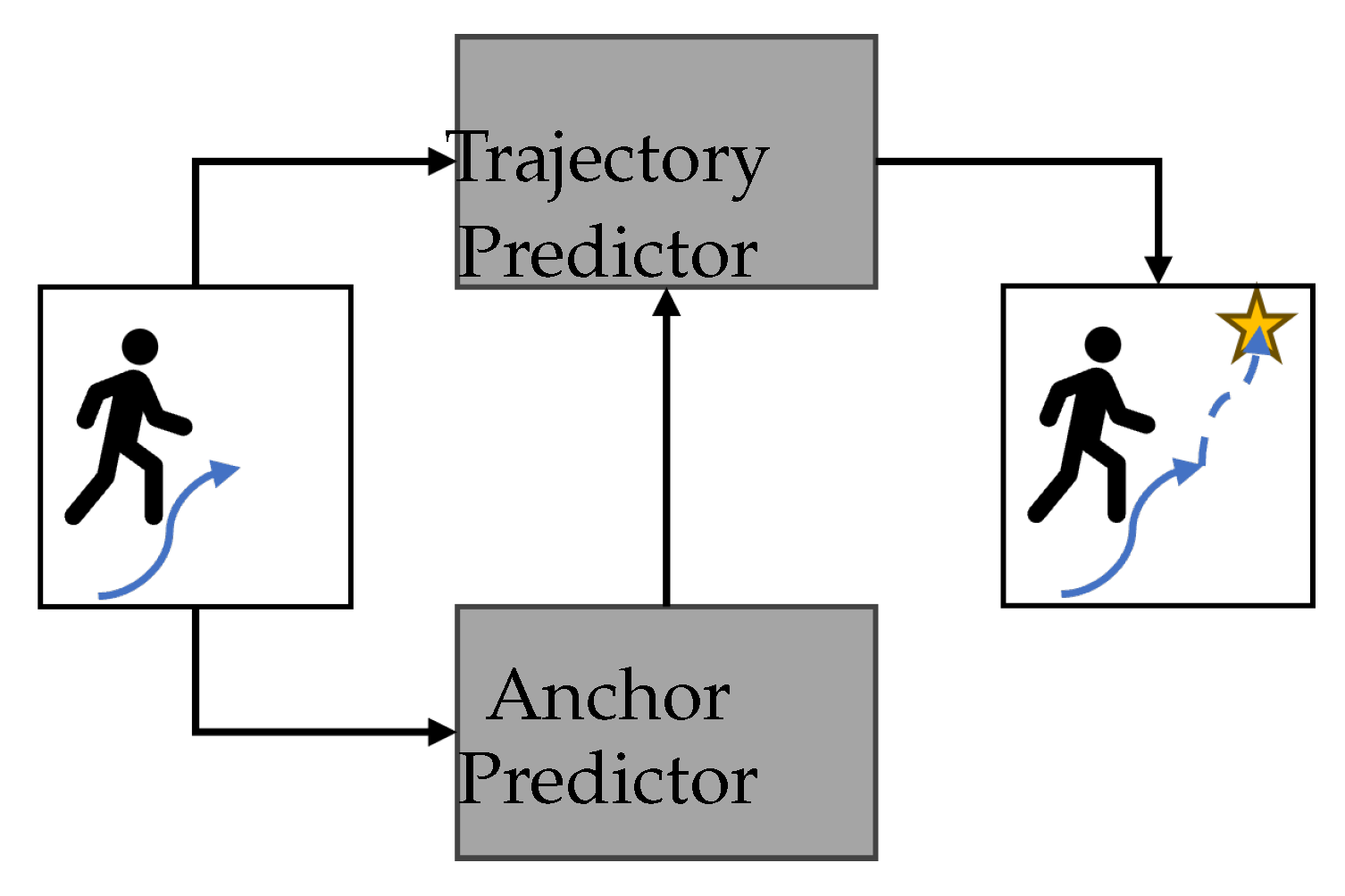
4.2. Anchor-Conditioned Methods

Anchor-conditioned models use a set of anchor points to condition the prediction of an agent’s trajectory [21,26,27,28,29,30,31]. These anchor points can be, for example, the respective agent’s estimated final goal position, which is used to condition the final trajectory estimation or even a trajectory proposal. The goal prediction module can be based on any of the other introduced prediction methods. The schematic for anchor-conditioned methods depicted in Figure 5 emphasizes this by showing the predictor as a black box. The goal prediction module uses the input to predict long-term goals for the targeted agents. The trajectory prediction module uses the goal prediction as additional input for its predictions.
Mangalam et al. [28] additionally used waypoints between the last observed positions and the estimated goal position. Here, the model predicted a probability distribution for both the goal and the interim waypoints. While Dendorfer et al. [30] modeled the multimodality of the task only through goal distribution estimation, which they argued eased the task of the trajectory decoder, Mangalam et al. [28] sampled goals and waypoints from the predicted distributions and generated a conditioned probability distribution for every timestep of the trajectory. Chiara et al. [26] followed this approach by sampling from goal distributions and injecting random noise into the trajectory generation module. While Mangalam et al. [28] performed their computations completely in image space, Chiara et al. [26] only predicted non-parametric probability distributions for possible goals in image space. The trajectory generation module was based on a recurrent network handling 2D positions of the agent of interest. Contrary to Dendorfer et al. [30] and Chiara et al. [26], who included scene information in the form of images only in their goal estimation module, Mangalam et al. [28] provided both their goal and waypoint module and their trajectory prediction module with an encoded segmentation map of the surroundings. Instead of directly predicting the goal probability distribution, Gu et al. [29] first scored the possible future lanes of the street network and then densely sampled goals based on this lane scoring. The probability of every goal was then calculated using the attention mechanism and a softmax function. Before using this set of goals, the authors applied a trainable goal set predictor to select the most likely goals. All methods introduced so far directly modeled position-based probability distributions and used them to sample possible goal positions for conditioning.
Zhang et al. [21] presented a goal-conditioned extension of AgentFormer [49] with ForceFormer. The authors extended the original architecture with a goal estimation module and a social force module. The goal estimation module estimated potential goals for agents, which were then fed into the social force and prediction (AgentFormer) module. The social force module modeled attractive and repulsive forces (goal and potential collisions) to make the predicted trajectories more socially acceptable and to model interactions. The additional features (social and goal) created in this way were supplied to AgentFormer by concatenating them with the positional sequences.
Li et al. [27] also modeled interactions in their goal prediction module by basing it on a GNN-encoded feature set of the surrounding agents and environment. Similarly to Gu et al. [29], the goal distributions were determined per estimated future lane.
ProphNet [22] follows a different approach to other anchor-conditioned methods. The method first generates proposals from the agent’s motion history (the sequence of positions, velocity, and heading) without constraints or conditioning to ensure a diverse and multimodal output of trajectories. ProphNet then generates anchors, i.e., goal positions, from encoded agent states, relative agent states (other agents), and road graphs. The M fused embeddings of anchors and proposals are used as inputs to N hydra prediction heads to produce N × M predicted trajectories, which are reduced to the required number of trajectories using NMS. The method relies on gated MLPs [117] instead of Transformers for encoding to achieve state-of-the-art inference times for agent-centric prediction methods.
Zhou et al. [23] used trajectory proposals as anchors in their method instead of goal estimates. For this, the authors presented a novel agent-centric representation that utilized agent features in polar coordinates, which were transformed into Fourier features. This formulation prevented the need for the recomputation of the agent-centric features at every timestep and was also rolled out to infrastructure elements. A DETR-inspired decoder [118] first generates proposal trajectories with learnable, anchor-free mode queries. The proposals are then used as anchors in the refinement module that uses learnable, anchor-based mode queries to compute deviations from the proposals and a likelihood for each hypothesis. The method outputs possible trajectories as a mixture of Laplace distributions.
Aydemir et al. [24] proposed a goal-conditioned method called ADAPT that could process scenes in agent-centric (marginal prediction) and scene-centric (joint prediction) manners using interchangeable endpoint prediction heads. ADAPT first generated scene graphs for lanes (from the HD map) and agents and encoded them using multi-head attention blocks with self- and cross-attention layers. This allowed the method to model agent–agent, agent–lane, and lane–lane interactions. The encoded features were used as input for the endpoint prediction module. The endpoint prediction module in scene-centric mode used a dynamic neural network [119] to adapt to the input state, thus allowing the network to adapt to each agent without having to iterate through each agent separately. In the agent-centric mode, the dynamic neural network was replaced by a simple MLP. In both modes, the endpoint proposals were refined using an MLP that predicted offsets for every endpoint. The final trajectory prediction was carried out by interpolating between the agent’s current position and the proposed goals.
Instead of relying on trajectory or goal proposals as anchors, Dong et al. [25] proposed sparse instance conditioning, essentially a mixture of both trajectory and goal conditioning. Their method used a memory module that stored sparse instances of future trajectories with observed trajectories as keys. This memory module was pre-trained using LSTM-based encoders and decoders. The second stage of the training focused on the memory refinement module, which was responsible for fine-tuning the retrieved sparse instances by applying two separate MLPs to generate deviation features and refined features. The refined features were concatenated with the encoded observed trajectories to generate the corresponding trajectory. During inference, the method retrieved more modes from memory than needed, which were then clustered to produce the required number of modes. This was carried out to reduce the mode redundancy of the sparse instances.

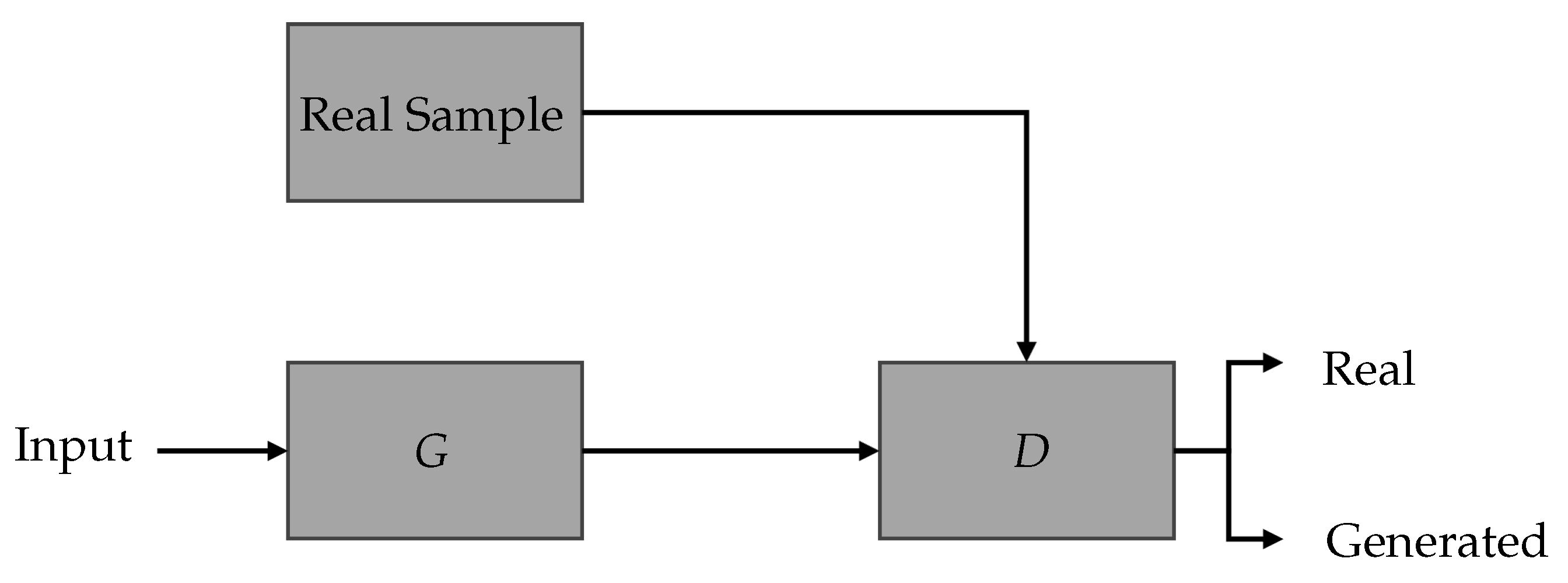
4.3. GAN-Based Methods

GANs consist of two neural networks trained simultaneously in opposition to each other in a minimax game. The two networks are a generator G that tries to capture the data distribution and generates samples and a discriminator D that estimates the probability that a sample came from the original training data or from G [120]. Figure 6 shows the basic architecture of a GAN. G takes as input a latent variable z and outputs sample G ( z ) , and D takes a sample x as input and outputs the probability D ( x ) , which leads to the objective function [37]:
min G max D V ( G , D ) = E x p d a t a ( x ) log D ( x ) + E z p ( z ) log ( 1 D ( G ( z ) ) ) .
GANs can also be conditioned on an additional input, e.g., past trajectories, which were used in the following methods.
Gupta et al. [37] first introduced the use of GANs for human trajectory prediction with SocialGAN. SocialGAN uses a simple LSTM-based generator that encodes past trajectories, passes the result through a social pooling module (see Section 3.2), and decodes the output to produce trajectories. Diversity and uncertainty are introduced by concatenating the output of the social pooling module with a random noise vector sampled from the standard distribution, which makes this method only unimodal. The encoder module is used as the discriminator to train the network adversarially.
The methods SocialBiGAT and SoPhie by Kosaraju et al. [36] and Sadeghian et al. [35] directly built on SocialGAN but offered significant improvement through scene and interaction modeling. SoPhie took over the overall structure of SocialGAN but replaced the social pooling module with an attention-based interaction module. The agent features were combined based on the relative distance between agent i and its surrounding agents. The inputs to the interaction module were the encoded features, the hidden states of the decoder module, and scene features extracted with a CNN from an image of the scene.
Kosaraju et al. [36] also changed how interactions were modeled in their method. SocialBiGAT models the interaction using a GAT [121] based on the LSTM-encoded features of the agents in the scene. Two discriminators supervise the adversarial training. The local discriminator is the same as in SocialGAN. In contrast, the global discriminator classifies the generated trajectories with respect to physical scene constraints extracted with a CNN from an image of the scene. Inspired by CycleGAN [122], the authors also introduced multimodality by training a latent encoder that mapped the generated trajectories back to the latent space. Wang et al. [32] applied the pedestrian-based SocialGAN architecture to highway scenarios for vehicles. For this, the interaction module was replaced by an autoencoder-based social module (see Section 3.2), while the rest of the overall structure stayed the same.
Li et al. [33] also applied adversarial training to the problem of pedestrian trajectory prediction but extracted trajectory features at different temporal resolutions using a pyramid network. The concatenated features were fused using a CNN before the trajectories were decoded. The model generated diverse trajectories by injecting unimodal noise in the generator module.
Zhou et al. [34] also extended the original SocialGAN with a state refinement module. This state refinement module replaced SocialGAN’s social pooling module with a GAT-based interaction module. This module placed all agents in groups and generated a scene graph based on intergroup, intragroup, and outgroup interactions between groups and agents within them. This allowed more fine-grained interaction modeling than with the proposed social pooling module.

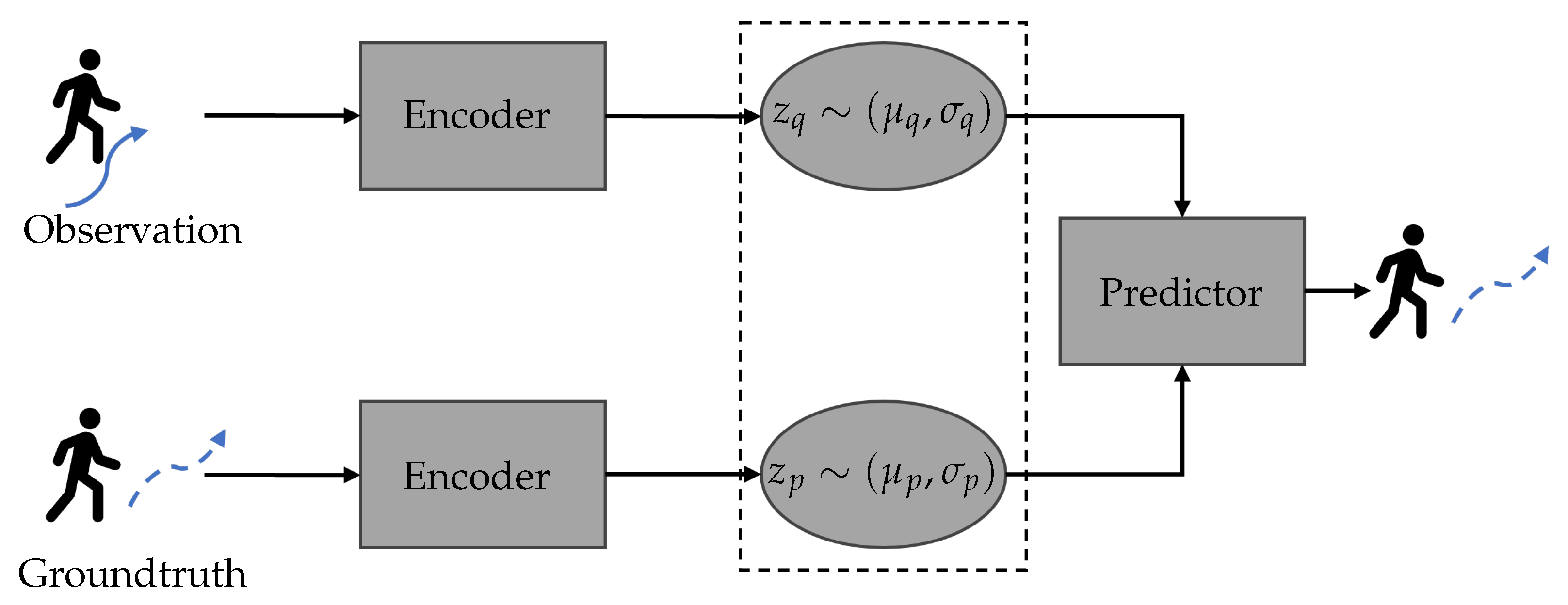
4.4. CVAE-Based Methods

Another generative model in addition to the GAN that is used for trajectory prediction is the CVAE. CVAEs are based on variational autoencoders that model input data x through a latent distribution q ( z | x ) by mapping x with a neural network. New data are generated by sampling from this latent distribution and decoding the resulting feature vector. CVAEs are conditioned on an additional input c and add a second network that maps a second latent distribution p ( z | c ) . In trajectory prediction, the CVAE is conditioned on past trajectory information, while q also incorporates the corresponding future trajectory. This is shown in Figure 7 as a schematic. The latent space modeled by the CVAE represents the latent distribution of the observed trajectories. The modeled distributions can be multimodal by having the CVAE predict multiple modes.
Zhu et al. [38] used a CVAE to map past trajectories and the ground-truth goal position into a joint probability distribution. Sampling from this distribution and concatenating these latent features with the encoded past trajectories served as the input for the trajectory predictor. The method also used a reciprocal consistency constraint by including a second network that mirrored the above-described prediction network. The mirror network took as an input the predicted trajectories and starting positions of each agent and predicted the observed trajectories. Both network parts were trained jointly. This helped stabilize the predictions of future trajectories and allowed the estimation of the prediction accuracy through a Pearson correlation coefficient-based metric without knowing the ground truth.
Closely related to this approach is BiTraP [48], which maps agent trajectories to a latent distribution using a GRU network. An MLP uses the sampled output to predict goal positions for the observed trajectories. A separate GRU network performs a forward prediction of the sampled output of the CVAE. The hidden layers, however, are not transformed into trajectories but rather used to initialize a backward GRU network that employs the predicted goal as a starting point and predicts the trajectory backward to the initial position from the goal.
Similar to this method, MUSE-VAE [42] uses a CVAE to predict the long-term goal of each agent in what the authors called the “Macro-stage”. The method then predicts waypoints based on the predicted long-term goal. Finally, the “Micro-stage” uses a second CVAE to predict future trajectories via the predicted long-term goals, the corresponding waypoints, and the encoded past trajectories. Features are extracted from positional heatmaps using convolutional U-Nets. As the bases for both the goal and the trajectory prediction are CVAEs, this method was classified into this category.
LSSTA [39] uses a much more complex encoder scheme on top of its CVAE. The observed agent trajectories are temporally encoded using a Transformer network and spatially encoded using a GCN. Both feature sets are fused with a TCN module before being concatenated with scene information extracted by a CNN from an image of the scene. This fused feature set consisting of scene information and temporal and spatial features is mapped into a latent space using a CVAE. The decoder is a simple MLP that predicts the future trajectory in an autoregressive manner. The CVAE is supervised by a parallel CVAE network that encodes only the observed trajectories using a GRU-based encoder. This idea influenced a more straightforward implementation by [123]. However, the authors of this method used a spatiotemporal graph that contained both spatial and temporal features.
Xie et al. [43] also carried out more sophisticated feature extraction by extracting spatial and temporal features separately. Additionally, they used a bi-directional decoder that predicted the future and past trajectories, thus alleviating the error accumulation problem with autoregressive methods. The CVAE was supervised by extracting the temporal features of future trajectories with the same temporal feature extractor.
Miguel et al. [44] also incorporated interactions separately into their VAE by encoding both relative positions and velocities between agents and position sequences of the agent of interest using LSTM networks. The VAE then predicted different distributions for the x- and y-positions of future trajectories.
Often, CVAEs only predict a unimodal latent distribution as a representation of possible future trajectories. Zhou et al. [40] tried to increase the expressiveness of the latent space using a cascade of CVAEs. Every CVAE predicted a single timestep of the trajectory and passed the predicted position onto the next CVAE. This autoregressive prediction scheme allowed the method to predict a separate latent distribution for the agent’s position at every timestep. The predicted trajectories were refined using a social pooling-based refinement module to make the trajectories socially acceptable. This module allowed the method to include future predictions in its interaction module.
In contrast to the above-mentioned methods, ScePT [16] uses a discrete CVAE to predict a discrete distribution over possible future trajectories. The latent space is represented by a Gibbs distribution sampled using a factor graph. Then, an autoregressive policy network first predicts the next future position and then ensures that the arising trajectory is realistic by applying an action network with a fixed dynamic model for the agent’s possible movements (vehicles and pedestrians).
Salzmann et al. [51] generated an agent-specific latent space by encoding the current scene using a graph-based representation encoded via LSTMs and attention layers. Like ScePT, the latent space was discrete and decoded using a set of GRU cells for every step. Each GRU cell produced a bivariate Gaussian distribution over the actions, which were combined with the agent’s system dynamics to produce the trajectory.
AgentFormer [49] uses a standard CVAE structure at its core but combines it with a modified Transformer for the encoding and decoding of features. As Transformers tend to lose temporal information and have no notion of agent identities for their attention mechanism, Yuan et al. [49] added temporal embeddings to their Transformer blocks and introduced agent-aware attention, which keeps track of an agent’s identity through masking and the use of two different query and key pairs per agent.
Xu et al. [41] used a VAE conditioned on the hidden states of an RNN at the core of their method. Their main focus was to address the problem of missing observations (e.g., due to occlusions) through simultaneous trajectory imputation and prediction. They encoded the current scene using three graph networks that employed different adjacency matrices. One network used a standard matrix that encoded connections with 0 and 1 together with a visibility matrix. The second matrix had a learnable adjacency matrix to learn the weights of connections between agents, and the final network used hot-encoded connection classes depending on the visibility of the connected nodes. The trajectories were decoded from the VAE’s hidden states.
Another interesting approach for pedestrian trajectory prediction was presented by Halawa et al. [46]. The authors proposed a bidirectional LSTM-based encoder–decoder structure extended from BiTraP [48] with a CVAE at its core. The main contribution of this method was its contrastive framework, which utilized action-based contrastive loss to train the encoder part to push trajectory embeddings of pedestrians performing the same action (the labels used were walking and standing) closer together. To generate enough positive and negative samples, synthetic trajectory samples generated by the CVAE were added to the samples of a given mini-batch. This sample generation process allowed the method to function without specific heuristics for negative mining. The method was able to produce multimodal outputs through its CVAE. Makansi et al. [124] showed that the idea of contrastive losses could also be applied to rare and difficult scenarios, making the network share cues present in these scenarios by pushing the embeddings of the trajectories closer together. A similar approach was presented by Liu et al. [125] with a focus on socially acceptable pedestrian trajectories without collisions, for which synthetically negative augmentation was used.
Choi and Min [47] proposed a CVAE that was supported by a GAN-based regularization mechanism. The core of this method was a two-level CVAE that produced a low-level latent variable to model each mode and a high-level latent variable to model the probabilities of the produced modes. Both parts used two lane-level context vectors generated by encoding state histories of the agents present in the scene via LSTMs and applying an attention mechanism to model interactions among agents and between agents and lanes. The model was trained with a discriminator network that regularized the shape of the predicted trajectory. Using the proposed two-level CVAE prevented mode blur, which would result in unrealistic predictions between lanes.

4.5. RNN-Based Methods

RNN-based networks like long short-term memory (LSTM) networks or gated recurrent units (GRUs) can also perform the task of trajectory prediction due to their Seq2Seq characteristic. Many of the introduced methods rely on RNNs at specific points. However, this chapter will introduce methods that use RNNs directly to predict future trajectories. PredictionNet by Kamenev et al. [54] relies on an image-based scene representation, as described in Section 3.2. It uses CNN encoders to encode the input images of the map, velocity, and occupancy into a latent vector that serves as the input for two RNNs: one for processing the observed velocities and occupancy and one for predicting the future. The hidden state of the RNNs is passed between timesteps, and the two RNNs after the observations are encoded to predict the future. The input to the future RNN is only the encoded current state of the velocity, occupancy, and map. This input provides a general, non-parametric representation of future traffic. Euler integration is applied to the output velocity tensor to provide discrete trajectories. The model is trained with simple focal loss for the occupancy and L 2 loss for the velocities.
Tang et al. [52], Sheng et al. [55], and Xu et al. [56] similarly applied RNN-based decoders. Their methods encoded the current scene with its agents into a spatiotemporal graph. Interactions at different temporal levels were extracted using a combination of GCNs and TCN layers. These encoded graph features were fed into an encoder–decoder trajectory generation module. While Tang et al. [52] used an LSTM-based generation module, Xu et al. [56] and Sheng et al. [55] opted for a GRU-based one.
Mo et al. [57] also applied the idea of encoding the scene with its agents and interactions using a graph. However, in this method, the feature processing in the graph was carried out using an edge-enhanced graph attention network. The processed features were decoded into trajectories using an LSTM. This method did not model multimodality and predicted future trajectories separately. The same approach was followed by Zhang et al. [53], who applied a GAT that was decoded to provide velocities for every timestep in an autoregressive manner using ConvGRUs.

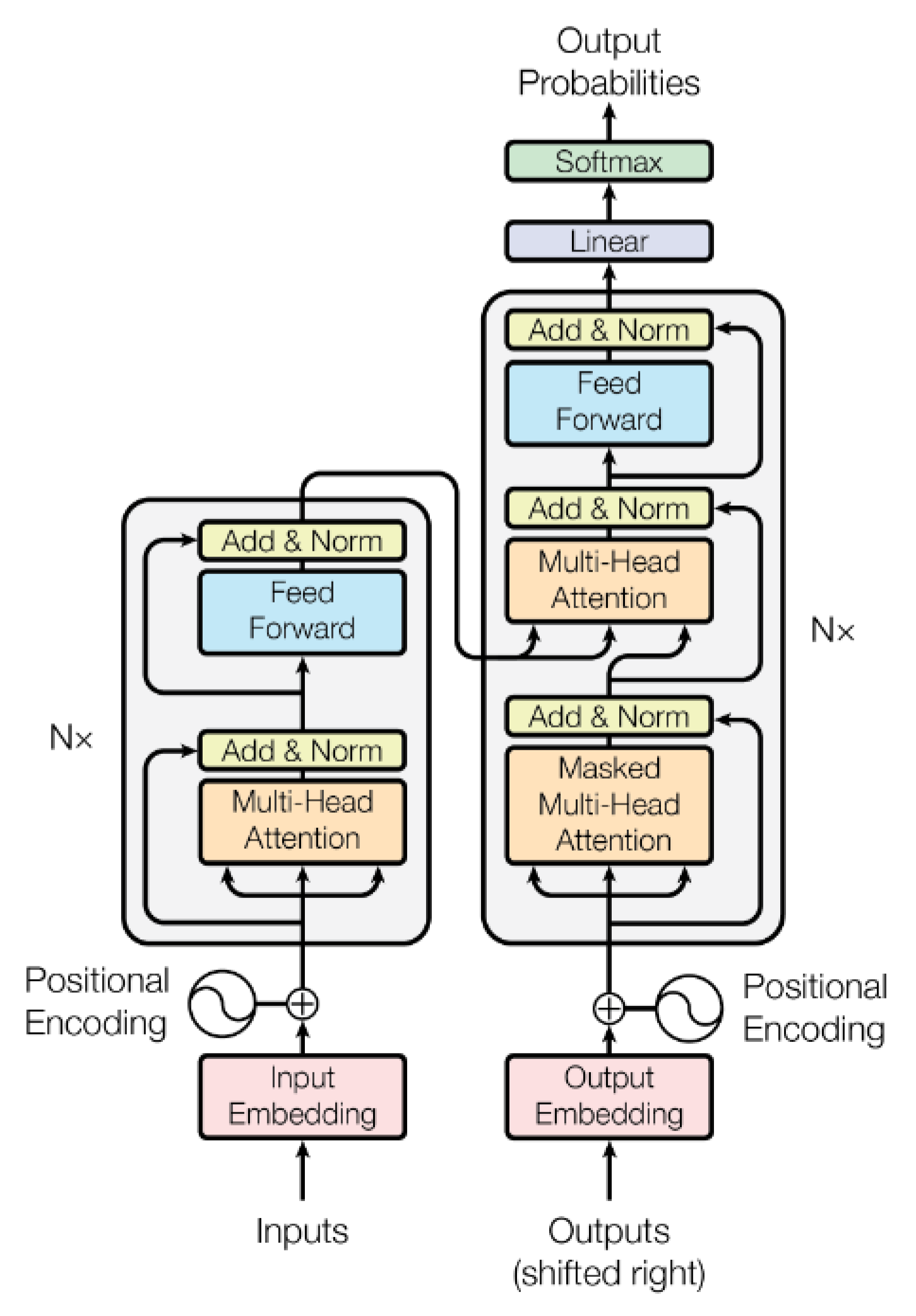
4.6. Transformer- and Attention-Based Methods

The Transformer [113] architecture is based on an attention mechanism, which helps to get rid of some of the disadvantages of RNNs like exploding or vanishing gradients by processing full sequences at once. It thus offers excellent sequence processing capabilities, which is why it is used in many trajectory prediction methods as the primary tool for generating predictions. One downside of Transformers is their quadratic complexity. The architecture is pictured in Figure 8.
Apart from methods that use the original Transformer architecture, this chapter will also introduce methods that use an attention mechanism to predict trajectories. The Transformer architecture can be used without any changes to predict trajectories based on observed positions [17,58,59,74,75,76].
Zhang et al. [58] applied two Transformers in parallel, one to infer obstacle positions from observed trajectories and one for predicting the x and y positions separately.
Liu et al. [59] used the embeddings of the last observed position as a query for the Transformer decoder part of the method, and Chen et al. [74] supported the training of their Transformer structure with a multitask learning scheme that trained the model on intention recognition and trajectory prediction.
Instead of predicting future positions directly, Shi et al. [75] designed their model to predict trajectories as GMMs to model the multimodality. With Transformers, multimodality can also be implicitly modeled using the output dimension of the Transformer, i.e., having the Transformer predict multiple trajectories per agent at once [17,76]. Another approach to using the Transformer in trajectory prediction is the use of Transformers for encoding, fusion, or interaction modeling. Here, standard MLPs are used to decode the latent space that is spanned by the Transformer encoding [60,69]. Multiple MLPs are used to generate multiple modes of trajectories. Schmidt et al. [70] followed this scheme for multimodality modeling but used a graph and soft attention for pre-processing the scene and its features.
Transformers can also be used just for decoding pre-processed scene features. Tsao et al. [71] used a Transformer decoder to decode encoded features of the agents and their interactions. The training was aided by two pretext tasks that predicted the interaction type and the closeness of two agents. The labels for these tasks were automatically generated; thus, a self-supervised approach was used.
Li et al. [72] applied a graph-based Transformer that used encoded node features as input and generated attention-based messages according to the graph structure. The Transformer predicted smooth and adapted trajectories using a memory replay module. Zhou et al. [73] extended the idea of VectorNet’s [110] form of representing agents and map features as vectors to a temporal Transformer. Multiple MLPs decoded the Transformer output to model multimodality.
Nayakanti et al. [62] presented a detailed ablation study with their method Wayformer. Wayformer consists of a Transformer-based encoder and decoder. In their paper, the authors showed that performing an early fusion with all input modalities (past positions, traffic light state, road graph, and interactions) together with a latent query-based attention mechanism delivered the best results. Using factorized (attention over time and space axes separately) or multiaxis (joint attention over time and space axes) attention did not influence the results significantly (Waymo Open Motion: m i n F D E difference, 0.001; m A P difference, 0.007; other metrics were equal).
Other methods do not directly apply Transformers but heavily rely on an attention mechanism for encoding and pre-processing the input data [61,67,68]. These features are decoded using RNN-based approaches [61] or MLPs [67,68]. Multimodality can also be modeled directly by predicting GMM components instead of directly predicting trajectories [67].
Gu et al. [63] introduced an end-to-end trajectory prediction approach that directly used multiview images as input. The method jointly detected, tracked, and predicted the positions of agents. For this, the authors applied 3D agent queries, which were updated using 3D-to-2D attention at every timestep, as in DETR3D [126]. The agent queries were used as input into the trajectory prediction module, which fused the queries with map features using attention. The latent and fused feature sets could be decoded into trajectories using regression, goal conditioning, or heatmap-based methods.
R-Pred [64] also employs queries in its processing pipeline. It consists of a proposal network that can be any multimodal trajectory prediction network. The M × N proposals for N agents, along with their features and confidence scores, serve as the input into the refinement network. This second stage first encodes elements from an HD map using a simple MLP and then pools these encoded features in tubular regions around the proposal trajectory’s waypoints. The pooled features and the proposal features are fused using a cross-attention block. A similar strategy is applied to model interactions between agents in the scene by first selecting close proposals and then applying cross-attention between the target proposals and the surrounding agents’ proposals. This ensures that future interactions are modeled and not only interactions based on observed positions. The final trajectory is generated by an MLP that predicts independent Laplace distributions using the concatenated features from scene and interaction processing.
TUTR [66] consists of a similar structure to Scene Transformer [17] and tackles the problem of pedestrian trajectory prediction with a simple Transformer encoder–decoder structure. TUTR uses a mode-level encoder that takes as input motion mode embeddings combined with observed trajectory embeddings. The motion mode embeddings are generated by clustering all future trajectories to C clusters and then projecting each cluster using a linear layer. Then, instead of supplying masked output embeddings to the decoder, TUTR uses the neighboring embeddings as input with the encoded motion modes and observed trajectories. The model uses a dual prediction head to predict future trajectories and their corresponding probabilities. Multimodality is modeled through the input of diverse motion modes into the encoder.
Zhu et al. [65] first encoded the scene using agent-centric, polyline-based coordinates and a Transformer encoder with relative positional encoding. The method then produced S static intentions by generating marginal predictions for each agent using M2I [15]. These intentions were fused using the authors’ Transformer-based high-level fusion module to decode goals and trajectory into K modes. A Transformer-based low-level fusion module further refined these predicted trajectories to output K scene-wide modes. Initially fusing high-level intentions and then refining these trajectories, as well as the agent-centric, polyline-based representation, allowed the method to take future interactions between agents into account and predict scene-wide and scene-consistent modes.

4.7. CNN-Based Methods

CNN-based methods predict agent trajectories on an image level instead of a coordinate level, as with other methods mentioned herein, and thereby rely on the popular convolutional layer. Mangalam et al. [28] used a simple CNN-based architecture; however, this method’s excellent performance could be traced back to its goal and waypoint conditioning, which is why the method is listed under Section 4.2. Wang et al. [77] used a temporal sequence of LiDAR point clouds as an input to their method. This sequence was encoded into a 2D pseudo-image in BEV with the image’s channels corresponding to the point cloud’s vertical dimension. The pseudo-images of every point cloud in the sequence were processed using 2D CNNs, where different concatenations of every timestep in the sequence encoded the temporal features. The fully encoded feature map of the given temporal sequence was upsampled, and a final CNN predicted the future movement of agents in the scene from a BEV. Zamboni et al. [78] followed a similar approach with coordinate-based input features instead of point clouds. The authors embedded the past positions of each agent into a 64-dimensional space and thus obtained a 64 × N t -dimensional, one-channel image, where N t is the number of observed positions. The paper discussed multiple ways to proceed with this input representation, including CoordConv [127] layers. However, the overall network architecture stayed the same: the pseudo-image was processed using several convolutional layers. A fully connected layer output the future positions based on the encoded convolutional features. Neither of the two above-mentioned CNN-based methods modeled the multimodality of the trajectory prediction task.

4.8. TCN-Based Methods

As depicted in Figure 9, TCNs make use of temporal convolutions, which apply the convolution operation across time instead of image space. The methods in this chapter utilize these to produce trajectory predictions.
All reviewed methods follow roughly the same network scheme [79,80,81,82,83,84]. First, the observed scenes are processed into a graph representation. Then, the graphs are processed using GCNs to extract features. These features are subsequently fed into a TCN-based decoder that produces the trajectory predictions for all agents in the scene. Lu et al. [82] and Lv et al. [79] also added scene context by extracting relevant features with a CNN encoder. Shi et al. [83] followed the method of Yang and Pei [39], introducing the division of spatial and temporal features and adding encoded temporal features to their spatial graph features before passing both to the TCN decoder. All methods except for the method of Bae and Jeon [84] applied some form of attention in their graph processing pipeline before passing the output to the decoder. Multimodality was not modeled in these methods.

4.9. Graph-Based Methods

This chapter introduces all reviewed methods that rely entirely on graph-based approaches like GCNs to predict future trajectories. Rowe et al. [85] modeled the scene using a sparse directed graph where interactions represented directed interactions between agents (nodes). This graph was pruned using an interaction classifier and turned into a directed acyclic graph (DAG) to decompose the joint prediction task into a series of marginal and conditional predictions for influencers and influenced agents. Predictions were made using a directed acyclic graph neural network [129] that decoded the node features into a sequence of future positions for each agent. Multimodality was introduced by passing N copies of the node features and a one-hot vector signifying the modality to the decoder.
GroupNet [87] is not a standalone trajectory prediction method. However, GroupNet offers an interesting take on graph formation for trajectory prediction. The method uses a multiscale hypergraph whose topology is learned during training. For this, an optimization problem of finding submatrices in the given affinity matrix of the initial hypergraph is solved. This optimization allows the graph to have both group-wise and individual interactions in a self-inferred topology. Neural message passing encodes the features in the graph, which can then be used by any prediction module to produce trajectory predictions. Combining this with, e.g., a CVAE (as in the above paper) allowed the method to model multimodality additionally.
Pourkeshavarz et al. [86] proposed an interesting method based on self-supervised meta-learning. In this method, the scene was encoded as a directed, heterogeneous information graph where infrastructure element nodes were initialized using a PointNet-based network and agent nodes were encoded using 1D convolutions. The authors applied Heterogeneous Graph Transformer (HGT) [130] as their GNN. They then performed joint meta-learning, where they first learned to find meta-paths between nodes that were not directly connected but could be reached with a series of steps between nodes. Next, they used these learned representations of the GNN to learn the main task of trajectory prediction and a set of auxiliary tasks, e.g., predicting the distance to the next intersection or maneuver classification. Additionally, the method learned to weigh the loss of the main and auxiliary tasks. This allowed the method to improve its map representational learning power for predicting possible future trajectories. The representations of a set of predefined meta-paths were used to model multimodality.

4.10. Set-Based Methods

Most of the methods introduced so far in this review directly predict trajectories or corresponding positional probability distributions in an unconstrained way, sometimes resulting in infeasible trajectory predictions [89,90].The methods in this chapter approach the problem of trajectory prediction with a two-step process. First, a set of trajectories is pre-generated, and then each sample in the set of trajectories is classified and scored according to contextual information [88,89,90]. This approach eases the task of trajectory prediction by avoiding mode collapse, eliminating dynamically infeasible trajectories beforehand, and ensuring a desired level of coverage of the possible trajectory state space [89]. However, this comes at the cost of the method’s expressiveness, since prior knowledge is introduced through the trajectory set generation.
Phan-Minh et al. [89] used both fixed and dynamic trajectory sets. The fixed trajectory set was simply generated by extracting trajectories from the training set, while the dynamic trajectory set made use of the current dynamic state of the agent of interest to generate possible trajectories by the forward integration of a dynamic model over diverse control sequences. The multimodal output for a single agent (marginal prediction) was generated by scoring the trajectories using dense layers.
To ensure both dynamic and environmental feasibility, Song et al. [90] proposed a more sophisticated trajectory generator. The method performed a depth-first search on an HD map to find reachable paths for the agent of interest. These paths were used as input for a Frenét planner [131] together with the initial dynamic state of the agent to produce dynamically and environmentally feasible trajectories. An evaluator that encoded state histories using LSTMs and attention to model past and future interactions between context entities (possible paths, state histories, and future trajectories) scored the proposed trajectories to produce joint, multimodal predictions.
Schmidt et al. [88] followed the approach of CoverNet [89] to produce a fixed trajectory set by using an algorithm to extract possible, type-specific (vehicle or VRU) trajectories from the complete dataset based on a metric (e.g., m i n A D E ). To predict trajectories for agents in the scene, the map, interaction, and past agent information was encoded, and an MLP finally predicted a probability for every trajectory in the previously generated set of trajectories depending on the class of the agent of interest. A simple non-maximum suppression selected the most likely trajectory. It discarded other trajectories with an endpoint within r N M S around the first trajectory’s endpoint until the desired number of modes was reached.

4.11. Other Prediction Methods

The methods in this chapter only partially fit into the other categories introduced so far. They apply either a novel or unique technique for trajectory prediction or offer a study on a topic surrounding trajectory prediction.
Bhatt et al. [91] offered an end-to-end approach for trajectory prediction. After performing 3D object detection and tracking, the authors generated a potential field for every object based on the extracted object states and HD map information. This potential field was used as a cost function to predict the velocities of agents in the scene. The trajectory could be deduced with the stepwise velocities (with magnitude as speed, and orientation as heading angle).
Wang et al. [95] also had a different take on trajectory prediction than the previously introduced methods. Instead of predicting trajectories per object, PointMotionNet predicts the movement of single points in its LiDAR input. For this, the authors turned the input point cloud sequence into a 4D point cloud and applied a 4D point spatiotemporal convolution in an encoder–decoder format to this point cloud. The decoder predicted a motion vector and a motion state per point.
Another end-to-end approach was proposed by Guo et al. [96]. The authors used the agents’ past trajectories and a BEV image of the scene to generate a reward map used in reinforcement learning. A value iteration network generated a multimodal policy map based on the generated reward map. Sampling from this policy map with the Gumbel-Softmax trick [132], an RNN generated the future position distribution from the high-level policy map plan. A Transformer-based refinement network sampled the predicted distribution to a few representative trajectories.
The method by Zernetsch et al. [97] is one of the few that dealt explicitly with predicting cyclist trajectories. The authors first extracted movement sequences through object detection and optical flow from image sequences. Then, basic movement detection was performed, where the observed movement was categorized as one of six movement forms (start, stop, left, right, move, and wait). Based on the detected movement form, form-specific networks predicted the movement probability distribution as a Gaussian distribution. Each of these probability distributions was combined to form an ensemble forecast of the future positions of the cyclist.
The next method to be presented in this chapter was presented by Monti et al. [98]. They published a study on reducing the dependence of methods on large numbers of observations (timesteps of observed trajectories). The authors applied a simple Transformer encoder–decoder structure with a teacher and student network. The teacher network was trained on eight observations, while the student network was trained on only two. Distillation loss was applied to let the student network closely follow the predictions of the teacher network. The authors showed that the student network could perform similarly to the teacher network while being trained on fewer observations. This insight is very viable for real-world applications where the number of observations is limited due to occlusions or sensing errors.
Sun et al. [15] relied on a two-step approach to produce joint predictions for two agents at a time. First, the interaction was classified into one of three classes: pass, yield, and none. Then, the trajectory of the influencer agent was marginally predicted, while the trajectory of the influenced agent was conditioned on the trajectory of the influencer. The authors applied a network of modules consisting of simple MLPs and ResNet structures.
Peri et al. [99] combined the problem of future trajectory prediction with object detection. For this, the authors approached the problem by taking a sequence of LiDAR point clouds as input and then detecting object classes in the scene. To predict the future trajectories of objects, they introduced object positions at future timesteps as classes, i.e., c a r t + 1 , c a r t + 2 , …, c a r t + k . This detection was independent of object detections in the current scene, which allowed the method to detect multiple possible future positions. Future positions were then backcasted to the current timestep and matched to object detections in the current scene through a distance metric, allowing many-to-one matching. All matched positions were scored by the detection confidence of the last predicted position in the trajectory. As the method relied on neither groundtruth detections nor external detections, it was able to learn important features of the input sensor data by itself and was closer to a real-world application than most other methods presented in this review.
Li et al. [92] followed a similar trajectory prediction approach to Peri et al. [99], using LiDAR points clouds directly as input. Instead of using object detection, the authors based their method on foreground/background segmentation with sparse labels. The approach consisted of a segmentation stage and a motion forecasting stage that associated consecutive foreground voxels with each other. To train the model, the authors proposed a novel outlier robust Chamfer distance loss formulation that incorporated three consecutive LiDAR frames to gauge the confidence of associated voxels. The advantage of this formulation was that it only needed sparse segmentation labels for training and no motion forecasting ground truth.
Chen et al. [93] proposed a self-supervised approach using masked autoencoders with Traj-MAE. Traj-MAE consists of a trajectory encoder, a map encoder, and a decoder based on AutoBot [133]. Both encoders were pre-trained with different masking strategies to learn how to efficiently encode both trajectories and map information. Trajectories were masked in their temporal and social dimensions, while map information was masked based on point, patch, and block levels. The pre-training was carried out in three stages with a mixture of all masking strategies to avoid forgetting crucial information.
Maeda and Ukita [94] proposed FlowChain, which is a density estimation model for trajectory prediction. FlowChain’s main architectural insight is a chain of conditional continuously indexed flows that transform the density of the previous timestep to the density of the next timestep and thus predict a density for every timestep in the prediction time frame. The first flow in this chain converts the Gaussian distribution of the newly observed position. This allows the density to change the topology of the base density. With every incoming observation, the model updates the densities at every timestep by replacing the first prediction with the new Gaussian density and then updating the remaining densities using the already computed flows. The model makes use of a temporal-social encoder to incorporate interactions and generate a motion trend, which is supplied to the flows. Trajectories can be generated by sampling from the computed densities. The main contribution of this method is its fast inference time due to its simple update scheme.
V2-Net [134] approaches the task of trajectory prediction not from a temporal sequence modeling point of view but from a spectral one. This method assumes that different frequency bands in the trajectory spectrum could represent an agent’s motion preferences. In this case, low-frequency bands could represent coarse agent goals, while high-frequency bands could represent finer motion variations as modeled by epistemic and aleatoric uncertainty. To model this, the authors proposed a two-network method that first predicted waypoints, which were then refined through spectral interpolation to produce agent trajectories. The model first applied a one-dimensional discrete Fourier Transform to each dimension of the observed trajectory sequence. An MLP then embedded these spectrums, which were afterward concatenated with a noise vector sampled from a normal distribution to model multimodality. A Transformer, together with the MLP, predicted waypoints of the trajectory in the spectral domain, which were used by another Transformer with CNN-encoded scene context (surroundings and social interactions) to predict the final trajectory. Transforming trajectories into the spectral domain allowed the display of smaller variations present in trajectories that were not visible when viewed in a positional domain.

5. Evaluation and Results

5.1. Datasets

The methods presented in this review were trained and evaluated using the ground truth of various datasets. These data were obtained using a variety of sensors, such as cameras and LiDARs, and by extracting trajectories from the obtained sensor material. Most datasets are divided into scenarios of fixed length and provide trajectory sequences or annotated bounding boxes for all agents in the scene. Autonomous driving datasets also provide raw sensor data as well as annotations for these data. As this review presents methods for trajectory prediction in autonomous driving scenarios and for VRUs, standard large-scale autonomous driving datasets and datasets for pedestrian trajectory prediction are introduced. The datasets used by methods in this review are listed in Table 2. HD maps are either rasterized or vectorized maps in the form of polylines. Some datasets like WOMD even include traffic signal states and the lanes they control [135]. While most datasets focus on single-agent marginal predictions, the benchmarks on Interaction and Argoverse 2 specifically incorporate scene-wide predictions (collision-free). As this review focuses on the methods themselves and not on the datasets, we refer the interested reader to the corresponding dataset papers for more information beyond this overview.

5.2. Metrics

This section will briefly overview commonly used evaluation metrics for trajectory prediction in autonomous driving and pedestrian trajectory prediction. All metrics are comparable over an equal prediction horizon, i.e., if the methods predict trajectories of an equal length.
Root Mean Square Error ( RMSE ): The RMSE calculates the square root of the average squared error between prediction y ^ and ground truth y:
R M S E = 1 T t = 1 T y t y ^ t 2 ,
where T denotes the number of predicted samples, and y and y ^ are positions extracted at timestep t.
Average Displacement Error ( ADE ): The A D E calculates the average L2-error between ground truth y and predicted position y ^ over all agents and timesteps. It is thus very similar to the RMSE. However, it allows an easier interpretation as the A D E is given in meters or pixels. The A D E is defined as follows:
A D E = 1 N 1 T n = 1 N t = 1 T y t n y ^ t n 2 ,
with N agents and T predicted timesteps. As many methods employ a multimodal output, i.e., predict multiple trajectories simultaneously, the A D E has to be slightly adapted. For this, m i n A D E k is introduced. This metric requires sampling or predicting k modes from the predicted multimodal output. m i n A D E k is the mode with the lowest A D E . Another extension of this metric is the brier m i n A D E k or b-minADEk. With this extension, the uncertainty estimation of the predicted trajectory is included beyond the sampling mechanism with
b - m i n A D E k = m i n A D E k 1 p 2 ,
where p is the probability score of the best-performing mode. Another extension is the extension as a joint or scene-wide metric, which includes the trajectories of all predicted agents in the scene at once.
Final Displacement Error ( FDE ): The F D E is very similar to the A D E metric, but instead of computing an average over the complete predicted trajectory, the F D E is only computed over the predicted endpoints y ^ T n . This can be formulated as
F D E = 1 N n = 1 N y T n y ^ T n 2 .
Multimodal extensions can be applied for the F D E in the same way as for the A D E , resulting in m i n F D E k and b-minFDEk over k predictions.
Miss Rate ( MR ): The M R is closely connected to the F D E . It provides the ratio of predictions where the F D E is bigger than 2 m [23]. Here, as for the A D E and F D E , a multimodal version M R k exists. This simply provides the M R of the best of k trajectories. The miss rate can also be set according to different criteria like longitudinal and lateral thresholds in order to, for example, model the structure of lanes [27].
Overlap Rate ( OR ): An overlap is defined for multi-agent scenarios in which the top-scoring predicted trajectories of two agents come so close at any timestep that their respective bounding boxes overlap. This can be seen as predicting a collision between these two agents, which is usually unrealistic. The overlap rate is the average overlaps over all timesteps. This is more commonly used in autonomous driving datasets.
Mean Average Precision ( mAP ): Some datasets (main ranking metric for WOMD [135]) employ the well-known m A P score for trajectory prediction. The m A P computes the area under the precision–recall curve by applying a confidence score threshold and using the M R to compute positive and negative predictions. Here, a positive prediction is defined by having an F D E < 2 and a negative prediction as an F D E > 2 . The m A P of WOMD is first computed for eight different trajectory shape types and then averaged over the same.

5.3. Summary of Reported Results

This section will concisely present the results of all methods introduced in this review sorted by dataset. This will give an overview of the methods and allow a direct comparison. Some papers reported results for multiple datasets, which is why these methods will be listed more than once. We refer the reader to the respective papers for details on the training parameters and settings. Results using datasets for which only one paper in this review reported results can be found in Appendix A. Table 3, Table 4, Table 5, Table 6, Table 7, Table 8, Table 9, Table 10, Table 11, Table 12, Table 13, Table 14 and Table 15 display the reported results of the methods introduced in Section 4. Individualized reports of results are indicated as best as possible. If a method was not given a name, we assigned one for the tables below. If not stated otherwise, the methods in the dataset tables below were trained under the same dataset settings (dataset splits, observation and prediction horizons, and number of sampled trajectories). Of course, this does not include model-specific hyperparameters like the learning rate or batch size. The methods reporting results on WOMD and nuScenes used many different settings (see Table 6 and Table 10), which made it hard to compare the results. We indicated deviations from the standard evaluation metrics mentioned in the tables through footnotes for each applicable method under every dataset table.

5.4. Discussion

This chapter will provide a short evaluation and discuss the presented methods. Through its separate, dedicated datasets (ETH/UCY and SDD) and methods, one can see that pedestrian trajectory prediction is still somewhat detached from trajectory prediction for autonomous driving in general. Only a subset of methods, e.g., ScePT [16] and Trajectron++ [51], presented results on both types of dataset (nuScenes and ETH/UCY). Both methods come from the CVAE class, which yielded state-of-the-art results on ETH/UCY, SDD, and nuScenes (see Table 3, Table 4, and Table 10). Most likely, this can be attributed to the excellent multimodality modeling capabilities of CVAEs. They can map their input to any parametric probability distribution and thus gain significant flexibility. Comparing the performance of different CVAEs on ETH/UCY (Table 3), one can see that the complex design choices of RCPNet [38] and LSSTA [39] described in Section 4.4 did not pay off compared to ScePT [16], which outperformed both of these methods with a simple graph-based encoding scheme using MLPs. One can also see that the cascaded CVAEs of CSR [40] benefitted the prediction of later timesteps, evident in its best overall m i n F D E 20 of 0.23. A similar trend can be seen with the two-level CVAE proposed by Choi and Min [47], which resulted in the best overall m i n A D E 6 on Argoverse 1. The good performance of the parametric distributions is contrasted by the performance of Y-Net [28], which achieved the maximum amount of flexibility by modeling occupancy probabilities with a non-parametric probability distribution. This flexibility allowed the method to achieve m i n A D E 20 and m i n F D E 20 values of 0.18 and 0.27, respectively, which made it the best-performing anchor-conditioned model on ETH/UCY (Table 3).
For the pedestrian datasets and Argoverse 1, anchor-conditioned models also showed outstanding performance metrics [21,23,25,26,28,29,31]. Again, their setup allows them to model multimodality very well. By estimating possible anchor points and refining their predicted trajectories conditioned on these anchors, they model epistemic and aleatoric uncertainty sequentially, thus following the route-finding mechanism of real-world agents (every agent has a long-term goal and reacts to events and the environment on the way). Additionally, though it is not reported in the tables of this review, Mangalam et al. [28] presented an interesting study on long-term prediction horizons using SDD with a time horizon of 30 s, showing remarkable performance. With an observation time of 1 s, Y-Net increased its m i n A D E 20 to only 14.99 compared to 7.85 for a time horizon of 4.8 s and an observation time of 3.2 s. This shows that the combination of goal anchors and waypoint anchors stabilized the trajectory prediction compared to an anchor-less method like S-GAN [37] that achieved a m i n A D E 20 of 38.57 in the same long-term setting. On the other hand, Transformers lagged slightly behind the previously mentioned classes on ETH/UCY and SDD (compare the results in Table 3 and Table 4). This most likely can be explained by their quadratic complexity and their need for large amounts of data, which might not be satisfied by the sizes of ETH/UCY and SDD [153,154]. While ETH/UCY and SDD only offer five and eight locations, respectively, the autonomous driving datasets offer many more, e.g., WOMD has 100,000 scenes of 20 s [106,107,155]. On these bigger datasets, the Transformer architecture is able to outperform other methods, as can be seen by MTR-A [75] and Wayformer [62] achieving the best overall results on WOMD. The attention mechanism and the original Transformer architecture also find uses along the complete prediction pipeline in encoders or for interaction modeling.
Diffusion models are a recent, interesting transfer of the diffusion process from image and text generation to the domain of trajectory prediction [18,19,20]. The introduced models showed good performance on ETH/UCY and SDD; however, they struggled with longer inference times. When evaluating 512 trajectories on the ZARA1 scene of the ETH/UCY dataset, Trajectron++ [51] needed 0.443 s, while MID took 17.368 s to process the same amount of trajectories [20]. This problem was partially addressed by Mao et al. [18] through their initialization strategy of the diffusion process. LED [18] and MID [20] showed competitive results on ETH/UCY and SDD (see Table 3 and Table 4), while MotionDiffuser only achieved an m A P of 0.20 compared to the values of 0.449 and 0.419 achieved by the leading Transformer architectures on WOMD [62,75]. This could be due to the higher diversity of the predicted trajectories resulting from the diffusion process, evident in the significantly higher M R of 0.43 (0.116 and 0.123 for MTR-A [75] and Wayformer [62], respectively).
GAN-based methods showed reasonable results on ETH/UCY [33,34,35,36,37] but remained mostly absent from autonomous driving datasets like nuScenes or WOMD (see Table 6 and Table 10). This may partly be due to the training difficulties of GANs, e.g., mode collapse, where the generator only learns to generate a small subset of samples that seem especially realistic to the discriminator [156,157]. Nevertheless, adversarial training still remains a promising future research direction if these training difficulties can be resolved. GANs also show flexibility with respect to their application, as demonstrated by Dendorfer et al. [30] with their Goal-GAN method, where they extended the GAN trajectory prediction structure to also include anchors. However, considering the results on SDD in Table 4, one can see that this integration is not very competitive and is in need of further tuning and research.
TCNs also showed competitive performance with the Transformer class on Interaction (Table 12) and ETH/UCY (Table 3) [79,80,81,82,83,84]. Considering the methods utilizing TCNs, one can see that the main application of TCNs in the setting of trajectory prediction is the decoding of high-dimensional, temporal graph features into trajectories. LSSTA [39] is at its core a CVAE but also makes use of TCNs in its encoding module. Through their ablation studies, the authors showed that TCNs can capture more details than a Transformer and process input sequences more efficiently than RNNs, which is evident in the promising results on ETH/UCY (see Table 3).
Graphs or GNNs are utilized in almost all methods in this review at some point in their architectural makeup. They are especially useful in modeling interactions through connections between agent nodes in the graph, which is essential for benchmarks like Argoverse 2 and Interaction that heavily focus on scene-consistent, and thus collision-free, trajectory predictions. However, comparing the results of graph-based methods (purely relying on graphs) shows that they generally only play a role in the middle of the performance field (compare the results on all presented datasets in Section 5.3). Thus, graphs are a significant asset for encoding scenes, but relying purely on GCNs to decode trajectories is insufficient to capture the inherent multimodality and complexity of future trajectories.
Another interesting direction taken by the authors of the ViP3D [63], PointMotionNet [95], and End-to-End [99] methods was the creation of an end-to-end pipeline that directly uses sensor input for its predictions. This, however, prevented a direct comparison of the achieved metrics, as these methods jointly detect and predict objects while other methods rely on the ground-truth positions provided by the datasets. Thus, one can question the real-world applicability of these methods in cars, as in most cases, it is not clear if the methods can handle inaccuracies and uncertainties in object positions caused by an upstream object detector.
One can see from Table 9 and Table 11 that all method classes struggled with increasing time horizons. However, considering speeds in urban environments, longer time horizons might not be necessary or realistic with respect to inference times. Also, with respect to the use of predictions in a downstream ego-motion planner, it might be enough to provide a non-parametric occupancy probability distribution, which would allow the thresholding of safe areas for the ego vehicle to drive on.

5.5. Potential Research Directions

This section will provide a brief overview of possible future research directions to improve and strengthen trajectory prediction in autonomous driving for vehicles and VRUs.
Joint and Scene-wide Predictions: Joint and scene-wide predictions are extremely important for predicting realistic trajectories in real-world scenarios. This necessitates modeling interactions not only in the scene encoding stage but also throughout the prediction process of future trajectories. Multimodal predictions result in scene-wide modes as the output is a connected probability distribution with all agents covered. ScePT [16] already incorporates this and shows excellent results, demonstrating that marginal predictions are less realistic than joint predictions. With benchmarks like Argoverse 2 and the 2023 Waymo Open Dataset Motion Prediction Challenge, which presents teams with the task of predicting up to eight agents for eight seconds simultaneously, the training and benchmarking capabilities are already present to improve models in this regard. Aleatoric uncertainty greatly influences how all traffic participants navigate their environment; thus, it is crucial to model this over the complete prediction horizon.
Input Features and Application: The choice of input features greatly impacts the performance of trajectory prediction methods. Map usage is ubiquitous in methods applied to larger autonomous driving datasets like nuScenes and WOMD (see references in Table 6 and Table 10). This helps increase the prediction quality as an agent’s environment significantly impacts their movement choices [110]. Closely connected to this is the incorporation of specific and explicit traffic rules, which has not been studied much in the context of trajectory prediction. This includes both the introduction of traffic signs and more high-level concepts like right of way or police-controlled intersections. Lin et al. [158] showed that incorporating traffic rules into a trajectory planning module helps generate rule-compliant trajectories for an ego vehicle. Transferring this approach to trajectory prediction models holds great promise for more rule-compliant predictions. Agent-specific features can also be investigated further regarding their impact on prediction quality. The pose of a VRU (both pedestrians and cyclists) can provide great insight into its future movements through viewing directions or concrete gestures by cyclists indicating their intent to turn. Human Scene Transformer [159] demonstrates this in an indoor setting. Its application to large datasets in the autonomous driving domain and the investigation of its concrete impacts on the quality of pedestrian predictions are still open questions. Additionally, including cyclist gestures in a Deep-Learning-based method remains to be achieved. Kooij et al. [160] examined specific cyclist scenarios with Dynamic Bayesian Networks and showed the benefit of using raised arms to indicate the cyclist’s intention to turn. The end-to-end methods introduced herein use either multiview images (ViP3D [63]) or LiDAR point clouds (End-to-End [99] and PointMotionNet [95]) as input, which leaves the combination of the two sensor modalities in an end-to-end method with a fusion approach open for future research. Tied together with end-to-end methods is the performance of trajectory prediction methods under uncertain inputs, i.e., with an upstream object detector. End-to-end methods jointly perform the two tasks, while the application of an object detector to most trajectory prediction methods has not been reported. The performance of the introduced methods without using the ground-truth object detections supplied by the dataset but instead employing an object detector remains questionable. Methods built for this particular application should make use of the object detector’s uncertainty estimates when predicting their trajectory uncertainties.
Generative and Foundation Models: With the advent of LLMs like GPT-4 [161] and their application to many different domains, research on their use as a trajectory prediction method remains largely open. Seff et al. [162] explored motion forecasting as a language modeling task in their recent paper. Their state-of-the-art WOMD results further proved that this is a promising research direction. Additionally, researching the explainability of multimodal predictions using LLMs would help increase the reliability and safety of prediction methods with respect to their later use in vehicles. Incorporating LLMs could also help implement active learning in an adversarial manner by allowing human feedback on possible predictions. Additionally, generative methods hold great promise for extending the reciprocal consistency constraints postulated by Zhu et al. [38] to not only positional data but also, e.g., the gestures and poses of VRUs. This leads to the next important topic, which is closely connected to the input features discussed in the previous paragraph. If novel methods employ more sophisticated input features, data augmentation becomes more difficult as rotations or translations will no longer be sufficient. For example, a valid augmentation of a scenario of a cyclist turning could be a cyclist who uses a gesture to indicate their intention or does not use a gesture. Augmentations like this can be achieved with models such as MotionGPT [163], which is able to generate realistic human motion applied to an SMPL model.
VRU Safety and Performance: Incorporating more fine-grained VRU classes is also a direction worth investigating as the dynamics within the greater VRU class can change drastically. Consider, for example, a person in a wheelchair and a walking adult, who move differently from each other. Also, maintaining model performance while reducing the inference time for real-world applications in vehicles should be an important aspect of future research. This includes investigations into the necessary time horizon for predictions and increasing the prediction accuracy for longer time horizons. A dynamically changing prediction horizon dependent on the speed, number of agents, and environmental state is also possible. Directly comparing models like this will be challenging. Nevertheless, increasing the model performance for predicting VRU movements is essential to reducing fatalities in traffic.
Data Availability and Domain Gaps: With the trend of ever more potent model architectures containing Transformers, the availability of data is key for training these models. That is why increasing the data availability, especially in challenging scenarios displaying interactions between infrastructure and heterogeneous agents, is very important for future research on trajectory prediction. As with data augmentation, mentioned above, artificially generating scenarios could be an interesting research direction. This could be exceptionally useful for dangerous or near-collision scenarios without endangering human life. The applicability of simulated scenarios together with real-world data is still an open issue for trajectory prediction methods. The impact of potential domain gaps in agent behavior, visual features, and rules between data recording locations also remains an open field of research worth investigating.

6. Conclusions

This paper conducted a thorough review of important Deep Learning methods in trajectory prediction for autonomous driving and VRUs. The review presented popular datasets, possible input features, ways to model interactions among agents, output representations, and multiple methods divided into several classes based on their primary prediction scheme. The postulated classes were diffusion-based, anchor-conditioned, GAN-based, CVAE-based, RNN-based, Transformer- and attention-based, CNN-based, TCN-based, graph-based, and set-based methods. Models that did not fit any of these classes but were still worth mentioning in this review were introduced under “Other”. Additionally, the reported results of the introduced methods were collected and summarized. A discussion of the performance and efficacy of the respective method classes followed the presentation of the reported results, which showed that CVAEs exhibit good performance on both pedestrian and autonomous driving datasets. On the other hand, Transformers lag behind CVAEs and anchor-conditioned methods on pedestrian datasets due to their quadratic complexity coupled with the dataset sizes. Last but not least, this review offered suggestions for future research directions regarding trajectory prediction methods in autonomous driving. Future research should focus on joint metrics and predictions, novel input features for end-to-end methods, and VRU safety. Additionally, investigating recent advances in generative and foundation models, as well as data availability and domain gaps between datasets, shows great promise for future research. This review should help in the future development of trajectory prediction methods by providing an easy way to compare and find corresponding methods and by facilitating the entrance into the vast field of Deep Learning methods in trajectory prediction for autonomous driving and VRUs.

Author Contributions

Conceptualization, E.S. and F.B.F.; methodology, E.S.; validation, E.S.; formal analysis, E.S.; investigation, E.S.; resources, E.S.; data curation, E.S.; writing—original draft preparation, E.S.; writing—review and editing, E.S. and F.B.F.; visualization, E.S.; supervision, F.B.F.; project administration, F.B.F.; funding acquisition, F.B.F. All authors have read and agreed to the published version of the manuscript.

Funding

This research was conducted within the project “Solutions and Technologies for Automated Driving in Town: an urban mobility project”, funded by the Federal Ministry for Economic Affairs and Climate Action (BMWK), based on a decision by the German Bundestag, grant no. 19A22006N.

Data Availability Statement

Data sharing not applicable.

Conflicts of Interest

The authors declare no conflict of interest. The funders had no role in the design of the study; in the collection, analyses, or interpretation of data; in the writing of the manuscript; or in the decision to publish the results.

Abbreviations

The following abbreviations are used in this manuscript:
GANGenerative adversarial network
CVAEConditional variational autoencoder
CNNConvolutional neural network
TCNTemporal convolutional network
GNNGraph neural network
LLMLarge Language Model
VRUVulnerable road user

Appendix A

This section contains the results of the methods introduced in this review on datasets for which no other paper presented in this review reported results.
Table A1. Unified results table for Lyft Level 5. The results are reported as A D E and F D E in meters. The method used a reduced version of this dataset (1000 agents).
MethodMethod ClassYear ADE FDE
Observations [98]Other20220.240.53
Table A2. Unified results table for VIRAT/ActEV. The results are reported as A D E and F D E in pixels.
MethodMethod ClassYear ADE FDE
Spatial Transformer [72]Transformer202218.5135.84
Table A3. Unified results table for KITTI. The results are reported as A D E and F D E at time horizons of 1 s and 3 s in meters.
MethodMethod ClassYear ADE @1 s ADE @3 s FDE @1 s FDE @3 s
PTP [123]CVAE20210.4711.3190.7632.299

References

  1. Zoox. Zoox Purpose-Built Robotaxi Is First in the World to Operate on Public Roads. 2023. Available online: https://zoox.com/wp-content/uploads/zoox-press-release-immediate-release.pdf (accessed on 9 October 2023).
  2. LLC, C. Human Ridehail Crash Rate Benchmark. 2023. Available online: https://getcruise.com/news/blog/2023/human-ridehail-crash-rate-benchmark/ (accessed on 9 October 2023).
  3. Lillo, L.D.; Gode, T.; Zhou, X.; Atzei, M.; Chen, R.; Victor, T. Comparative Safety Performance of Autonomous- and Human Drivers: A Real-World Case Study of the Waymo One Service. arXiv 2023, arXiv:2309.01206. [Google Scholar]
  4. Laumond, J.; Sekhavat, S.; Lamiraux, F. Lecture Notes in Control and Information Sciences 229; Springer: Berlin/Heidelberg, Germany, 1998. [Google Scholar]
  5. Foundation, C.V. CVPR 2023 Open Access. 2023. Available online: https://openaccess.thecvf.com/CVPR2023?day=all (accessed on 24 October 2023).
  6. Foundation, C.V. ICCV 2023 Open Access. 2023. Available online: https://openaccess.thecvf.com/ICCV2023?day=all (accessed on 24 October 2023).
  7. Leon, F.; Gavrilescu, M. A review of tracking and trajectory prediction methods for autonomous driving. Mathematics 2021, 9, 660. [Google Scholar] [CrossRef]
  8. Liu, J.; Mao, X.; Fang, Y.; Zhu, D.; Meng, M.Q.H. A survey on deep-learning approaches for vehicle trajectory prediction in autonomous driving. In Proceedings of the IEEE International Conference on Robotics and Biomimetics (ROBIO), Sanya, China, 6–9 December 2021; IEEE: Piscataway, NJ, USA, 2021; pp. 978–985. [Google Scholar]
  9. Huang, Y.; Du, J.; Yang, Z.; Zhou, Z.; Zhang, L.; Chen, H. A survey on trajectory-prediction methods for autonomous driving. IEEE Trans. Intell. Veh. 2022, 7, 652–674. [Google Scholar] [CrossRef]
  10. Ridel, D.; Rehder, E.; Lauer, M.; Stiller, C.; Wolf, D. A literature review on the prediction of pedestrian behavior in urban scenarios. In Proceedings of the International Conference on Intelligent Transportation Systems (ITSC), Maui, HI, USA, 4–7 November 2018; IEEE: Piscataway, NJ, USA, 2018; pp. 3105–3112. [Google Scholar]
  11. Rudenko, A.; Palmieri, L.; Herman, M.; Kitani, K.M.; Gavrila, D.M.; Arras, K.O. Human motion trajectory prediction: A survey. Int. J. Robot. Res. 2020, 39, 895–935. [Google Scholar] [CrossRef]
  12. Graves, A. Generating Sequences with Recurrent Neural Networks. arXiv 2013, arXiv:1308.0850. [Google Scholar]
  13. O’Mahony, N.; Campbell, S.; Carvalho, A.; Harapanahalli, S.; Hernandez, G.V.; Krpalkova, L.; Riordan, D.; Walsh, J. Deep Learning vs. Traditional Computer Vision. In Proceedings of the Computer Vision Conference (CVC), Online, 14–19 June 2020; pp. 128–144. [Google Scholar]
  14. Trenn, S. Multilayer Perceptrons: Approximation Order and Necessary Number of Hidden Units. IEEE Trans. Neural Netw. 2008, 19, 836–844. [Google Scholar] [CrossRef]
  15. Sun, Q.; Huang, X.; Gu, J.; Williams, B.C.; Zhao, H. M2I: From Factored Marginal Trajectory Prediction to Interactive Prediction. In Proceedings of the IEEE/CVF Conference on Computer Vision and Pattern Recognition (CVPR), New Orleans, LA, USA, 18–24 June 2022; pp. 6543–6552. [Google Scholar]
  16. Chen, Y.; Ivanovic, B.; Pavone, M. Scept: Scene-consistent, policy-based trajectory predictions for planning. In Proceedings of the IEEE/CVF Conference on Computer Vision and Pattern Recognition (CVPR), New Orleans, LA, USA, 18–24 June 2022; pp. 17103–17112. [Google Scholar]
  17. Ngiam, J.; Caine, B.; Vasudevan, V.; Zhang, Z.; Chiang, H.T.L.; Ling, J.; Roelofs, R.; Bewley, A.; Liu, C.; Venugopal, A.; et al. Scene transformer: A unified architecture for predicting future trajectories of multiple agents. In Proceedings of the International Conference on Learning Representations (ICLR), Virtual, 25–29 April 2022. [Google Scholar]
  18. Mao, W.; Xu, C.; Zhu, Q.; Chen, S.; Wang, Y. Leapfrog Diffusion Model for Stochastic Trajectory Prediction. In Proceedings of the IEEE/CVF Conference on Computer Vision and Pattern Recognition (CVPR), Vancouver, BC, Canada, 18–22 June 2023; pp. 5517–5526. [Google Scholar]
  19. Jiang, C.M.; Cornman, A.; Park, C.; Sapp, B.; Zhou, Y.; Anguelov, D. MotionDiffuser Controllable Multi-Agent Motion Prediction Using Diffusion. In Proceedings of the IEEE/CVF Conference on Computer Vision and Pattern Recognition (CVPR), Vancouver, BC, Canada, 18–22 June 2023; pp. 9644–9653. [Google Scholar]
  20. Gu, T.; Chen, G.; Li, J.; Lin, C.; Rao, Y.; Zhou, J.; Lu, J. Stochastic Trajectory Prediction via Motion Indeterminacy Diffusion. In Proceedings of the IEEE/CVF Conference on Computer Vision and Pattern Recognition (CVPR), New Orleans, LA, USA, 18–24 June 2022; pp. 17092–17101. [Google Scholar]
  21. Zhang, W.; Cheng, H.; Johora, F.T.; Sester, M. ForceFormer: Exploring Social Force and Transformer for Pedestrian Trajectory Prediction. arXiv 2023, arXiv:2302.07583. [Google Scholar]
  22. Wang, X.; Su, T.; Da, F.; Yang, X. ProphNet: Efficient Agent-Centric Motion Forecasting with Anchor-Informed Proposals. In Proceedings of the IEEE/CVF Conference on Computer Vision and Pattern Recognition (CVPR), Vancouver, BC, Canada, 18–22 June 2023; pp. 21995–22003. [Google Scholar]
  23. Zhou, Z.; Wang, J.; Li, Y.H.; Huang, Y.K. Query-Centric Trajectory Prediction. In Proceedings of the IEEE/CVF Conference on Computer Vision and Pattern Recognition (CVPR), Vancouver, BC, Canada, 18–22 June 2023; pp. 17863–17873. [Google Scholar]
  24. Aydemir, G.; Akan, A.K.; Güney, F. ADAPT: Efficient Multi-Agent Trajectory Prediction with Adaptation. In Proceedings of the IEEE/CVF International Conference on Computer Vision (ICCV), Paris, France, 2–6 October 2023; pp. 8295–8305. [Google Scholar]
  25. Dong, Y.; Wang, L.; Zhou, S.; Hua, G. Sparse Instance Conditioned Multimodal Trajectory Prediction. In Proceedings of the IEEE/CVF International Conference on Computer Vision (ICCV), Paris, France, 2–6 October 2023; pp. 9763–9772. [Google Scholar]
  26. Chiara, L.F.; Coscia, P.; Das, S.; Calderara, S.; Cucchiara, R.; Ballan, L. Goal-Driven Self-Attentive Recurrent Networks for Trajectory Prediction. In Proceedings of the IEEE/CVF Conference on Computer Vision and Pattern Recognition (CVPR) Workshops, New Orleans, LA, USA, 18–24 June 2022; pp. 2518–2527. [Google Scholar]
  27. Li, D.; Zhang, Q.; Lu, S.; Pan, Y.; Zhao, D. Conditional Goal-oriented Trajectory Prediction for Interacting Vehicles with Vectorized Representation. IEEE Trans. Neural Netw. Learn. Syst. 2021, 1–13. [Google Scholar] [CrossRef]
  28. Mangalam, K.; An, Y.; Girase, H.; Malik, J. From Goals, Waypoints and Paths to Long Term Human Trajectory Forecasting. In Proceedings of the IEEE/CVF International Conference on Computer Vision (ICCV), Virtual, 11–17 October 2021; pp. 15233–15242. [Google Scholar]
  29. Gu, J.; Sun, C.; Zhao, H. Densetnt: End-to-end trajectory prediction from dense goal sets. In Proceedings of the IEEE/CVF International Conference on Computer Vision (ICCV), Virtual, 11–17 October 2021; pp. 15303–15312. [Google Scholar]
  30. Dendorfer, P.; Osep, A.; Leal-Taixe, L. Goal-GAN: Multimodal Trajectory Prediction Based on Goal Position Estimation. In Proceedings of the Asian Conference on Computer Vision (ACCV), Kyoto, Japan, 30 November–4 December 2020. [Google Scholar]
  31. Mangalam, K.; Girase, H.; Agarwal, S.; Lee, K.H.; Adeli, E.; Malik, J.; Gaidon, A. It Is Not the Journey But the Destination Endpoint Conditioned Trajectory Prediction. In Proceedings of the European Conference on Computer Vision (ECCV), Glasgow, UK, 23–28 August 2020; pp. 759–776. [Google Scholar]
  32. Wang, Y.; Zhao, S.; Zhang, R.; Cheng, X.; Yang, L. Multi-Vehicle Collaborative Learning for Trajectory Prediction with Spatio-Temporal Tensor Fusion. IEEE Trans. Intell. Transp. Syst. 2022, 23, 236–248. [Google Scholar] [CrossRef]
  33. Li, Y.; Liang, R.; Wei, W.; Wang, W.; Zhou, J.; Li, X. Temporal pyramid network with spatial-temporal attention for pedestrian trajectory prediction. IEEE Trans. Netw. Sci. Eng. 2022, 9, 1006–1019. [Google Scholar] [CrossRef]
  34. Zhou, L.; Zhao, Y.; Yang, D.; Liu, J. GCHGAT: Pedestrian trajectory prediction using group constrained hierarchical graph attention networks. Appl. Intell. 2022, 52, 11434–11447. [Google Scholar] [CrossRef]
  35. Sadeghian, A.; Kosaraju, V.; Sadeghian, A.; Hirose, N.; Rezatofighi, S.H.; Savarese, S. SoPhie: An Attentive GAN for Predicting Paths Compliant to Social and Physical Constraints. In Proceedings of the IEEE/CVF Conference on Computer Vision and Pattern Recognition (CVPR), Long Beach, CA, USA, 15–20 June 2019; pp. 1349–1358. [Google Scholar]
  36. Kosaraju, V.; Sadeghian, A.; Martín-Martín, R.; Reid, I.; Rezatofighi, S.H.; Savarese, S. Social-bigat: Multimodal trajectory forecasting using bicycle-gan and graph attention networks. In Proceedings of the Advances in Neural Information Processing Systems (NeurIPS), Vancouver, BC, Canada, 8–14 December 2019. [Google Scholar]
  37. Gupta, A.; Johnson, J.; Fei-Fei, L.; Savarese, S.; Alahi, A. Social GAN: Socially Acceptable Trajectories with Generative Adversarial Networks. In Proceedings of the IEEE/CVF Conference on Computer Vision and Pattern Recognition (CVPR), Salt Lake City, UT, USA, 18–23 June 2018; pp. 2255–2264. [Google Scholar]
  38. Zhu, W.; Liu, Y.; Zhang, M.; Yi, Y. Reciprocal Consistency Prediction Network for Multi-Step Human Trajectory Prediction. IEEE Trans. Intell. Transp. Syst. 2023, 24, 6042–6052. [Google Scholar] [CrossRef]
  39. Yang, C.; Pei, Z. Long-Short Term Spatio-Temporal Aggregation for Trajectory Prediction. IEEE Trans. Intell. Transp. Syst. 2023, 24, 4114–4126. [Google Scholar] [CrossRef]
  40. Zhou, H.; Ren, D.; Yang, X.; Fan, M.; Huang, H. CSR: Cascade Conditional Variational Auto Encoder with Socially-aware Regression for Pedestrian Trajectory Prediction. Pattern Recognit. 2023, 133, 109030. [Google Scholar] [CrossRef]
  41. Xu, Y.; Bazarjani, A.; Chi, H.-g.; Choi, C.; Fu, Y. Uncovering the Missing Pattern: Unified Framework Towards Trajectory Imputation and Prediction. In Proceedings of the IEEE/CVF Conference on Computer Vision and Pattern Recognition (CVPR), Vancouver, BC, Canada, 18–22 June 2023; pp. 9632–9643. [Google Scholar]
  42. Lee, M.; Sohn, S.S.; Moon, S.; Yoon, S.; Kapadia, M.; Pavlovic, V. MUSE-VAE: Multi-Scale VAE for Environment-Aware Long Term Trajectory Prediction. In Proceedings of the IEEE/CVF Conference on Computer Vision and Pattern Recognition (CVPR), New Orleans, LA, USA, 18–24 June 2022; pp. 2221–2230. [Google Scholar]
  43. Xie, C.; Li, Y.; Liang, R.; Dong, L.; Li, X. Synchronous Bi-Directional Pedestrian Trajectory Prediction with Error Compensation. In Proceedings of the Asian Conference on Computer Vision (ACCV), Macau, China, 4–8 December 2022; pp. 2796–2812. [Google Scholar]
  44. Miguel, M.A.D.; Armingol, J.M.; Garcia, F. Vehicles Trajectory Prediction Using Recurrent VAE Network. IEEE Access 2022, 10, 32742–32749. [Google Scholar] [CrossRef]
  45. Su, Z.; Huang, G.; Zhang, S.; Hua, W. Crossmodal Transformer Based Generative Framework for Pedestrian Trajectory Prediction. In Proceedings of the IEEE International Conference on Robotics and Automation (ICRA), Philadelphia, PA, USA, 23–27 May 2022; pp. 2337–2343. [Google Scholar]
  46. Halawa, M.; Hellwich, O.; Bideau, P. Action-based Contrastive Learning for Trajectory Prediction. In Proceedings of the European Conference on Computer Vision (ECCV), Tel Aviv, Israel, 23–27 October 2022; pp. 143–159. [Google Scholar]
  47. Choi, D.; Min, K. Hierarchical Latent Structure for Multi-modal Vehicle Trajectory Forecasting. In Proceedings of the European Conference on Computer Vision (ECCV), Tel Aviv, Israel, 23–27 October 2022; pp. 129–145. [Google Scholar]
  48. Yao, Y.; Atkins, E.; Johnson-Roberson, M.; Vasudevan, R.; Du, X. BiTraP: Bi-Directional Pedestrian Trajectory Prediction with Multi-Modal Goal Estimation. IEEE Robot. Autom. Lett. 2021, 6, 1463–1470. [Google Scholar] [CrossRef]
  49. Yuan, Y.; Weng, X.; Kitani, K.M. Agentformer: Agent-aware transformers for socio-temporal multi-agent forecasting. In Proceedings of the IEEE/CVF International Conference on Computer Vision (ICCV), Virtual, 11–17 October 2021; pp. 9813–9823. [Google Scholar]
  50. Weng, X.; Wang, J.; Levine, S.; Kitani, K.; Rhinehart, N. Inverting the Pose Forecasting Pipeline with SPF2: Sequential Pointcloud Forecasting for Sequential Pose Forecasting. In Proceedings of the Proceedings of Machine Learning Research, PMLR, 10, Virtual, 8–10 September 2021; pp. 11–20. [Google Scholar]
  51. Salzmann, T.; Ivanovic, B.; Chakravarty, P.; Pavone, M. Trajectron++: Dynamically-Feasible Trajectory Forecasting with Heterogeneous Data. In Proceedings of the European Conference on Computer Vision (ECCV), Glasgow, UK, 23–28 August 2020; Springer Science and Business Media Deutschland GmbH: Berlin/Heidelberg, Germany, 2020; pp. 683–700. [Google Scholar]
  52. Tang, L.; Yan, F.; Zou, B.; Li, W.; Lv, C.; Wang, K. Trajectory prediction for autonomous driving based on multiscale spatial-temporal graph. IET Intell. Transp. Syst. 2023, 17, 386–399. [Google Scholar] [CrossRef]
  53. Zhang, K.; Zhao, L.; Dong, C.; Wu, L.; Zheng, L. AI-TP: Attention-Based Interaction-Aware Trajectory Prediction for Autonomous Driving. IEEE Trans. Intell. Veh. 2023, 8, 73–83. [Google Scholar] [CrossRef]
  54. Kamenev, A.; Wang, L.; Bohan, O.B.; Kulkarni, I.; Kartal, B.; Molchanov, A.; Birchfield, S.; Nister, D.; Smolyanskiy, N. PredictionNet: Real-Time Joint Probabilistic Traffic Prediction for Planning, Control, and Simulation. In Proceedings of the IEEE International Conference on Robotics and Automation (ICRA), Philadelphia, PA, USA, 23–27 May 2022; pp. 8936–8942. [Google Scholar]
  55. Sheng, Z.; Xu, Y.; Xue, S.; Li, D. Graph-Based Spatial-Temporal Convolutional Network for Vehicle Trajectory Prediction in Autonomous Driving. IEEE Trans. Intell. Transp. Syst. 2022, 23, 17654–17665. [Google Scholar] [CrossRef]
  56. Xu, D.; Shang, X.; Liu, Y.; Peng, H.; Li, H. Group Vehicle Trajectory Prediction with Global Spatio-Temporal Graph. IEEE Trans. Intell. Veh. 2022, 8, 1219–1229. [Google Scholar] [CrossRef]
  57. Mo, X.; Huang, Z.; Xing, Y.; Lv, C. Multi-agent trajectory prediction with heterogeneous edge-enhanced graph attention network. IEEE Trans. Intell. Transp. Syst. 2022, 23, 9554–9567. [Google Scholar] [CrossRef]
  58. Zhang, W.; Chai, Q.; Zhang, Q.; Wu, C. Obstacle-transformer: A trajectory prediction network based on surrounding trajectories. IET Cyber-Syst. Robot. 2023, 5, e12066. [Google Scholar] [CrossRef]
  59. Liu, D.; Li, Q.; Li, S.; Kong, J.; Qi, M. Non-Autoregressive Sparse Transformer Networks for Pedestrian Trajectory Prediction. Appl. Sci. 2023, 13, 3296. [Google Scholar] [CrossRef]
  60. Wang, Z.; Guo, J.; Hu, Z.; Zhang, H.; Zhang, J.; Pu, J. Lane Transformer: A High-Efficiency Trajectory Prediction Model. IEEE Open J. Intell. Transp. Syst. 2023, 4, 2–13. [Google Scholar] [CrossRef]
  61. Chen, H.; Liu, Y.; Hu, C.; Zhang, X. Vulnerable Road User Trajectory Prediction for Autonomous Driving Using a Data-Driven Integrated Approach. IEEE Trans. Intell. Transp. Syst. 2023, 24, 7306–7317. [Google Scholar] [CrossRef]
  62. Nayakanti, N.; Al-Rfou, R.; Zhou, A.; Goel, K.; Refaat, K.S.; Sapp, B. Wayformer Motion Forecasting via Simple & Efficient Attention Networks. In Proceedings of the IEEE International Conference on Robotics and Automation (ICRA), London, UK, 29 May–2 June 2023; pp. 2980–2987. [Google Scholar]
  63. Gu, J.; Hu, C.; Zhang, T.; Chen, X.; Wang, Y.; Wang, Y.; Zhao, H.; University, T.; Zhi, S.Q. ViP3D: End-to-End Visual Trajectory Prediction via 3D Agent Queries. In Proceedings of the IEEE/CVF Conference on Computer Vision and Pattern Recognition (CVPR), Vancouver, BC, Canada, 18–22 June 2023; pp. 5496–5506. [Google Scholar]
  64. Choi, S.; Kim, J.; Yun, J.; Choi, J.W. R-Pred: Two-Stage Motion Prediction Via Tube-Query Attention-Based Trajectory Refinement. In Proceedings of the IEEE/CVF International Conference on Computer Vision (ICCV), Paris, France, 2–6 October 2023; pp. 8525–8535. [Google Scholar]
  65. Zhu, Y.; Luan, D.; Shen, S. BiFF: Bi-level Future Fusion with Polyline-based Coordinate for Interactive Trajectory Prediction. In Proceedings of the IEEE/CVF International Conference on Computer Vision (ICCV), Paris, France, 2–6 October 2023; pp. 8260–8271. [Google Scholar]
  66. Shi, L.; Wang, L.; Zhou, S.; Hua, G. Trajectory Unified Transformer for Pedestrian Trajectory Prediction. In Proceedings of the IEEE/CVF International Conference on Computer Vision (ICCV), Paris, France, 2–6 October 2023; pp. 9675–9684. [Google Scholar]
  67. Duan, J.; Wang, L.; Long, C.; Zhou, S.; Zheng, F.; Shi, L.; Huan, G. Complementary Attention Gated Network for Pedestrian Trajectory Prediction. In Proceedings of the AAAI Conference on Artificial Intelligence, Vancouver, BC, Canada, 28 February–1 March 2022; pp. 542–550. [Google Scholar]
  68. Wang, J.; Ye, T.; Gu, Z.; Chen, J. LTP: Lane-based Trajectory Prediction for Autonomous Driving. In Proceedings of the IEEE/CVF Conference on Computer Vision and Pattern Recognition (CVPR), New Orleans, LA, USA, 18–24 June 2022; pp. 17134–17142. [Google Scholar]
  69. Huang, Z.; Mo, X.; Lv, C. Multi-modal Motion Prediction with Transformer-based Neural Network for Autonomous Driving. In Proceedings of the IEEE International Conference on Robotics and Automation (ICRA), Philadelphia, PA, USA, 23–27 May 2022; pp. 2605–2611. [Google Scholar]
  70. Schmidt, J.; Jordan, J.; Gritschneder, F.; Dietmayer, K. CRAT-Pred: Vehicle Trajectory Prediction with Crystal Graph Convolutional Neural Networks and Multi-Head Self-Attention. In Proceedings of the International Conference on Robotics and Automation (ICRA), Philadelphia, PA, USA, 23–27 May 2022; pp. 7799–7805. [Google Scholar]
  71. Tsao, L.W.; Wang, Y.K.; Lin, H.S.; Shuai, H.H.; Wong, L.K.; Cheng, W.H. Social-SSL: Self-supervised Cross-Sequence Representation Learning Based on Transformers for Multi-agent Trajectory Prediction. In Proceedings of the European Conference on Computer Vision (ECCV), Tel Aviv, Israel, 23–27 October 2022; pp. 234–250. [Google Scholar]
  72. Li, L.; Pagnucco, M.; Song, Y. Graph-based spatial transformer with memory replay for multi-future pedestrian trajectory prediction. In Proceedings of the IEEE/CVF Conference on Computer Vision and Pattern Recognition (CVPR), New Orleans, LA, USA, 18–24 June 2022; pp. 2231–2241. [Google Scholar]
  73. Zhou, Z.; Ye, L.; Wang, J.; Wu, K.; Lu, K. HiVT: Hierarchical Vector Transformer for Multi-Agent Motion Prediction. In Proceedings of the IEEE/CVF Conference on Computer Vision and Pattern Recognition (CVPR), New Orleans, LA, USA, 18–24 June 2022; pp. 8823–8833. [Google Scholar]
  74. Chen, X.; Zhang, H.; Zhao, F.; Cai, Y.; Wang, H.; Ye, Q. Vehicle Trajectory Prediction Based on Intention-Aware Non-Autoregressive Transformer with Multi-Attention Learning for Internet of Vehicles. IEEE Trans. Instrum. Meas. 2022, 71, 2513912. [Google Scholar] [CrossRef]
  75. Shi, S.; Jiang, L.; Dai, D.; Schiele, B. MTR-A: 1st Place Solution for 2022 Waymo Open Dataset Challenge–Motion Prediction. arXiv 2022, arXiv:2209.10033. [Google Scholar] [CrossRef]
  76. Sun, H.; Sun, F. Social-Transformer: Pedestrian Trajectory Prediction in Autonomous Driving Scenes. In Proceedings of the International Conference on Cognitive Systems and Signal Processing (ICCSIP), Suzhou, China, 20–21 November 2021; Springer Science and Business Media Deutschland GmbH: Berlin/Heidelberg, Germany, 2021; pp. 177–190. [Google Scholar]
  77. Wang, Y.; Pan, H.; Zhu, J.; Wu, Y.H.; Zhan, X.; Jiang, K.; Yang, D. BE-STI: Spatial-Temporal Integrated Network for Class-Agnostic Motion Prediction with Bidirectional Enhancement. In Proceedings of the IEEE/CVF Conference on Computer Vision and Pattern Recognition (CVPR), New Orleans, LA, USA, 18–24 June 2022; pp. 17093–17102. [Google Scholar]
  78. Zamboni, S.; Kefato, Z.T.; Girdzijauskas, S.; Noren, C.; Col, L.D. Pedestrian trajectory prediction with convolutional neural networks. Pattern Recognit. 2022, 121, 108252. [Google Scholar] [CrossRef]
  79. Lv, P.; Wang, W.; Wang, Y.; Zhang, Y.; Xu, M.; Xu, C. SSAGCN: Social Soft Attention Graph Convolution Network for Pedestrian Trajectory Prediction. IEEE Trans. Neural Netw. Learn. Syst. 2023, 1–15. [Google Scholar] [CrossRef]
  80. Lian, J.; Ren, W.; Li, L.; Zhou, Y.; Zhou, B. PTP-STGCN: Pedestrian Trajectory Prediction Based on a Spatio-temporal Graph Convolutional Neural Network. Appl. Intell. 2023, 53, 2862–2878. [Google Scholar] [CrossRef]
  81. Sighencea, I.B.; Stanciu, R.I.; Caleanu, D.C. D-STGCN: Dynamic Pedestrian Trajectory Prediction UsingSpatio-Temporal Graph Convolutional Networks. Electronics 2023, 12, 611. [Google Scholar] [CrossRef]
  82. Lu, Y.; Wang, W.; Hu, X.; Xu, P.; Zhou, S.; Cai, M. Vehicle Trajectory Prediction in Connected Environments via Heterogeneous Context-Aware Graph Convolutional Networks. IEEE Trans. Intell. Transp. Syst. 2023, 24, 8452–8464. [Google Scholar] [CrossRef]
  83. Shi, L.; Wang, L.; Long, C.; Zhou, S.; Zhou, M.; Niu, Z.; Hua, G. SGCN: Sparse Graph Convolution Network for Pedestrian Trajectory Prediction. In Proceedings of the IEEE/CVF Conference on Computer Vision and Pattern Recognition (CVPR), Nashville, TN, USA, 20–25 June 2021; pp. 8994–9003. [Google Scholar]
  84. Bae, I.; Jeon, H.G. Disentangled Multi-Relational Graph Convolutional Network for Pedestrian Trajectory Prediction. In Proceedings of the AAAI Conference on Artificial Intelligence, Virtual, 8–9 February 2021; pp. 911–919. [Google Scholar]
  85. Rowe, L.; Ethier, M.; Dykhne, E.H.; Czarnecki, K. FJMP: Factorized Joint Multi-Agent Motion Prediction over Learned Directed Acyclic Interaction Graphs. In Proceedings of the IEEE/CVF Conference on Computer Vision and Pattern Recognition (CVPR), Vancouver, BC, Canada, 18–22 June 2023. [Google Scholar]
  86. Pourkeshavarz, M.; Chen, C.; Ark, R.N.; Lab, H.; Toronto, C. Learn TAROT with MENTOR: A Meta-Learned Self-Supervised Approach for Trajectory Prediction. In Proceedings of the IEEE/CVF International Conference on Computer Vision (ICCV), Paris, France, 2–6 October 2023; pp. 8384–8393. [Google Scholar]
  87. Xu, C.; Li, M.; Ni, Z.; Zhang, Y.; Chen, S. GroupNet: Multiscale Hypergraph Neural Networks for Trajectory Prediction with Relational Reasoning. In Proceedings of the IEEE/CVF Conference on Computer Vision and Pattern Recognition (CVPR), New Orleans, LA, USA, 18–24 June 2022; pp. 6498–6507. [Google Scholar]
  88. Schmidt, J.; Huissel, P.; Wiederer, J.; Jordan, J.; Belagiannis, V.; Dietmayer, K. RESET: Revisiting Trajectory Sets for Conditional Behavior Prediction. In Proceedings of the IEEE Intelligent Vehicles Symposium (IV), Anchorage, AK, USA, 4–7 June 2023. [Google Scholar]
  89. Phan-Minh, T.; Grigore, E.C.; Boulton, F.A.; Beijbom, O.; Wolff, E.M. CoverNet: Multimodal Behavior Prediction using Trajectory Sets. In Proceedings of the IEEE/CVF Conference on Computer Vision and Pattern Recognition (CVPR), Seattle, WA, USA, 13–19 June 2020; pp. 14074–14083. [Google Scholar]
  90. Song, H.; Luan, D.; Ding, W.; Wang, M.Y.; Chen, Q. Learning to Predict Vehicle Trajectories with Model-based Planning. In Proceedings of the Conference on Robot Learning, Auckland, New Zealand, 14–18 December 2022; pp. 1035–1045. [Google Scholar]
  91. Bhatt, N.P.; Khajepour, A.; Hashemi, E. MPC-PF: Socially and Spatially Aware Object Trajectory Prediction for Autonomous Driving Systems Using Potential Fields. IEEE Trans. Intell. Transp. Syst. 2023, 24, 5351–6361. [Google Scholar] [CrossRef]
  92. Li, R.; Shi, H.; Fu, Z.; Wang, Z.; Lin, G. Weakly Supervised Class-Agnostic Motion Prediction for Autonomous Driving. In Proceedings of the IEEE/CVF Conference on Computer Vision and Pattern Recognition (CVPR), Vancouver, BC, Canada, 18–22 June 2023; pp. 17599–17608. [Google Scholar]
  93. Chen, H.; Wang, J.; Shao, K.; Liu, F.; Hao, J.; Guan, C.; Chen, G.; Heng, P.A. Traj-MAE: Masked Autoencoders for Trajectory Prediction. In Proceedings of the IEEE/CVF International Conference on Computer Vision (ICCV), Paris, France, 2–6 October 2023; pp. 8351–8362. [Google Scholar]
  94. Maeda, T.; Ukita, N. Fast Inference and Update of Probabilistic Density Estimation on Trajectory Prediction. In Proceedings of the IEEE/CVF International Conference on Computer Vision (ICCV), Paris, France, 2–6 October 2023; pp. 9795–9805. [Google Scholar]
  95. Wang, J.; Li, X.; Sullivan, A.; Abbott, L.; Chen, S. PointMotionNet: Point-Wise Motion Learning for Large-Scale LiDAR Point Clouds Sequences. In Proceedings of the IEEE/CVF Conference on Computer Vision and Pattern Recognition (CVPR), New Orleans, LA, USA, 18–24 June 2022; pp. 4419–4428. [Google Scholar]
  96. Guo, K.; Liu, W.; Pan, J. End-to-End Trajectory Distribution Prediction Based on Occupancy Grid Maps. In Proceedings of the IEEE/CVF Conference on Computer Vision and Pattern Recognition (CVPR), New Orleans, LA, USA, 18–24 June 2022; pp. 2242–2251. [Google Scholar]
  97. Zernetsch, S.; Reichert, H.; Kress, V.; Doll, K.; Sick, B. A Holistic View on Probabilistic Trajectory Forecasting—Case Study. Cyclist Intention Detection. In Proceedings of the IEEE Intelligent Vehicles Symposium (IV), Aachen, Germany, 4–9 June 2022; pp. 265–272. [Google Scholar]
  98. Monti, A.; Porrello, A.; Calderara, S.; Coscia, P.; Ballan, L.; Cucchiara, R. How Many Observations Are Enough? Knowledge Distillation for Trajectory Forecasting. In Proceedings of the IEEE/CVF Conference on Computer Vision and Pattern Recognition (CVPR), New Orleans, LA, USA, 18–24 June 2022; pp. 6553–6562. [Google Scholar]
  99. Peri, N.; Luiten, J.; Li, M.; Ošep, A.; Leal-Taixé, L.; Ramanan, D. Forecasting From LiDAR via Future Object Detection. In Proceedings of the IEEE/CVF Conference on Computer Vision and Pattern Recognition, New Orleans, LA, USA, 18–24 June 2022; pp. 17202–17211. [Google Scholar]
  100. Agarwal, A.; Lalit, M.; Bansal, A.; Seeja, K. iSGAN: An Improved SGAN for Crowd Trajectory Prediction from Surveillance Videos. Procedia Comput. Sci. 2023, 218, 2319–2327. [Google Scholar] [CrossRef]
  101. Casas, S.; Sadat, A.; Urtasun, R. MP3: A Unified Model To Map, Perceive, Predict and Plan. In Proceedings of the IEEE/CVF Conference on Computer Vision and Pattern Recognition (CVPR), Nashville, TN, USA, 20–25 June 2021; pp. 14403–14412. [Google Scholar]
  102. Chen, H.; Liu, Y.; Zhao, B.; Hu, C.; Zhang, X. Vision-based Real-time Online Vulnerable Traffic Participants Trajectory Prediction for Autonomous Vehicle. IEEE Trans. Intell. Veh. 2023, 8, 2110–2122. [Google Scholar] [CrossRef]
  103. Chen, X.; Zhang, H.; Zhao, F.; Hu, Y.; Tan, C.; Yang, J. Intention-Aware Vehicle Trajectory Prediction Based on Spatial-Temporal Dynamic Attention Network for Internet of Vehicles. IEEE Trans. Intell. Transp. Syst. 2022, 23, 19471–19483. [Google Scholar] [CrossRef]
  104. Huynh, M.; Alaghband, G. Online Adaptive Temporal Memory with Certainty Estimation for Human Trajectory Prediction. In Proceedings of the IEEE/CVF Winter Conference on Applications of Computer Vision (WACV), Waikoloa, HI, USA, 2–7 January 2023; pp. 940–949. [Google Scholar]
  105. Kress, V.; Jeske, F.; Zernetsch, S.; Doll, K.; Sick, B. Pose and Semantic Map Based Probabilistic Forecast of Vulnerable Road Users Trajectories. IEEE Trans. Intell. Veh. 2022, 8, 2592–2603. [Google Scholar] [CrossRef]
  106. Lerner, A.; Chrysanthou, Y.; Lischinski, D. Crowds by Example. Comput. Graph. Forum 2007, 26, 655–664. [Google Scholar] [CrossRef]
  107. Pellegrini, S.; Ess, A.; Schindler, K.; Van Gool, L. You’ll Never Walk Alone: Modeling Social Behavior for Multi-target Tracking. In Proceedings of the IEEE International Conference on Computer Vision, Kyoto, Japan, 29 September–2 October 2009; pp. 261–268. [Google Scholar]
  108. Robicquet, A.; Sadeghian, A.; Alahi, A.; Savarese, S. Learning Social Etiquette: Human Trajectory Prediction in Crowded Scenes. In Proceedings of the European Conference on Computer Vision (ECCV), Amsterdam, The Netherlands, 11–14 October 2016; pp. 21–37. [Google Scholar]
  109. Wu, C.; Chen, Y.; Luo, J.; Su, C.C.; Dawane, A.; Hanzra, B.; Deng, Z.; Liu, B.; Wang, J.Z.; Kuo, C.-h. MEBOW: Monocular Estimation of Body Orientation in the Wild. In Proceedings of the IEEE/CVF Conference on Computer Vision and Pattern Recognition (CVPR), Seattle, WA, USA, 13–19 June 2020; pp. 3451–3461. [Google Scholar]
  110. Gao, J.; Sun, C.; Zhao, H.; Shen, Y.; Anguelov, D.; Li, C.; Schmid, C. VectorNet: Encoding HD Maps and Agent Dynamics from Vectorized Representation. In Proceedings of the IEEE/CVF Conference on Computer Vision and Pattern Recognition (CVPR), Seattle, WA, USA, 13–19 June 2020; pp. 11525–11533. [Google Scholar]
  111. Schmidt, J.; Jordan, J.; Gritschneder, F.; Monninger, T.; Dietmayer, K. Exploring Navigation Maps for Learning-Based Motion Prediction. In Proceedings of the IEEE International Conference on Robotics and Automation (ICRA), London, UK, 29 May–2 June 2023. [Google Scholar]
  112. Liang, M.; Yang, B.; Hu, R.; Chen, Y.; Liao, R.; Feng, S.; Urtasun, R. Learning Lane Graph Representations for Motion Forecasting. In Proceedings of the European Conference on Computer Vision (ECCV), Glasgow, UK, 23–28 August 2020; pp. 541–556. [Google Scholar]
  113. Vaswani, A.; Shazeer, N.; Parmar, N.; Uszkoreit, J.; Jones, L.; Gomez, A.N.; Kaiser, Ł.; Polosukhin, I. Attention is all you need. In Proceedings of the Advances in Neural Information Processing Systems (NeurIPS), Long Beach, CA, USA, 4–9 December 2017. [Google Scholar]
  114. Bae, I.; Park, J.H.; Jeon, H.G. Non-Probability Sampling Network for Stochastic Human Trajectory Prediction. In Proceedings of the IEEE/CVF Conference on Computer Vision and Pattern Recognition (CVPR), New Orleans, LA, USA, 18–24 June 2022; pp. 6477–6487. [Google Scholar]
  115. Rombach, R.; Blattmann, A.; Lorenz, D.; Esser, P.; Ommer, B. High-Resolution Image Synthesis with Latent Diffusion Models. In Proceedings of the IEEE/CVF Conference on Computer Vision and Pattern Recognition (CVPR), New Orleans, LA, USA, 18–24 June 2022; pp. 10684–10695. [Google Scholar]
  116. Croitoru, F.A.; Hondru, V.; Ionescu, R.T.; Shah, M. Diffusion Models in Vision: A Survey. IEEE Trans. Pattern Anal. Mach. Intell. 2023, 45, 10850–10869. [Google Scholar] [CrossRef]
  117. Liu, H.; Dai, Z.; So, D.; Le, Q.V. Pay Attention to MLPs. In Proceedings of the Advances in Neural Information Processing Systems (NeurIPS), Virtual, 6–14 December 2021; pp. 9204–9215. [Google Scholar]
  118. Carion, N.; Massa, F.; Synnaeve, G.; Usunier, N.; Kirillov, A.; Zagoruyko, S. End-to-End Object Detection with Transformers. In Proceedings of the European Conference on Computer Vision (ECCV), Glasgow, UK, 23–28 August 2020; pp. 213–229. [Google Scholar]
  119. Han, Y.; Huang, G.; Song, S.; Yang, L.; Wang, H.; Wang, Y. Dynamic Neural Networks: A Survey. IEEE Trans. Pattern Anal. Mach. Intell. (TPAMI) 2021, 44, 7436–7456. [Google Scholar] [CrossRef]
  120. Goodfellow, I.; Pouget-Abadie, J.; Mirza, M.; Xu, B.; Warde-Farley, D.; Ozair, S.; Courville, A.; Bengio, Y. Generative Adversarial Nets. In Proceedings of the Advances in Neural Information Processing Systems (NeurIPS), Montreal, QC, Canada, 8–13 December 2014. [Google Scholar]
  121. Velickovic, P.; Cucurull, G.; Casanova, A.; Romero, A.; Liò, P.; Bengio, Y. Graph attention networks. In Proceedings of the International Conference on Learning Representations (ICLR), New Orleans, LA, USA, 6–9 May 2019. [Google Scholar]
  122. Zhu, J.Y.; Park, T.; Isola, P.; Efros, A.A. Unpaired Image-To-Image Translation Using Cycle-Consistent Adversarial Networks. In Proceedings of the IEEE International Conference on Computer Vision (ICCV), Venice, Italy, 22–29 October 2017; pp. 2223–2232. [Google Scholar]
  123. Weng, X.; Yuan, Y.; Kitani, K. PTP: Parallelized Tracking and Prediction with Graph Neural Networks and Diversity Sampling. IEEE Robot. Autom. Lett. 2021, 6, 4640–4647. [Google Scholar] [CrossRef]
  124. Makansi, O.; Cicek, Ö.; Marrakchi, Y.; Brox, T. On Exposing the Challenging Long Tail in Future Prediction of Traffic Actors. In Proceedings of the IEEE/CVF International Conference on Computer Vision (ICCV), Virtual, 11–17 October 2021; pp. 13147–13157. [Google Scholar]
  125. Liu, Y.; Yan, Q.; Alahi, A. Social NCE: Contrastive Learning of Socially-Aware Motion Representations. In Proceedings of the IEEE/CVF International Conference on Computer Vision (ICCV), Virtual, 11–17 October 2021; pp. 15118–15129. [Google Scholar]
  126. Wang, Y.; Guizilini, V.C.; Zhang, T.; Wang, Y.; Zhao, H.; Solomon, J. DETR3D: 3D Object Detection from Multi-View Images via 3D-to-2D Queries. In Proceedings of the Conference on Robot Learning, PMLR, Auckland, New Zealand, 14–18 December 2022; pp. 180–191. [Google Scholar]
  127. Liu, R.; Lehman, J.; Molino, P.; Petroski Such, F.; Frank, E.; Sergeev, A.; Yosinski, J. An intriguing failing of convolutional neural networks and the coordconv solution. In Proceedings of the Advances in Neural Information Processing Systems (NeurIPS), Montréal, QC, Canada, 3–8 December 2018. [Google Scholar]
  128. Bai, S.; Kolter, J.Z.; Koltun, V. An empirical evaluation of generic convolutional and recurrent networks for sequence modeling. arXiv 2018, arXiv:1803.01271. [Google Scholar]
  129. Thost, V.; Chen, J. Directed Acyclic Graph Neural Networks. In Proceedings of the International Conference on Learning Representations (ICLR), Virtual, 3–7 May 2021. [Google Scholar]
  130. Hu, Z.; Dong, Y.; Wang, K.; Sun, Y. Heterogeneous Graph Transformer. In Proceedings of the Web Conference, Taipei, Taiwan, 20–24 April 2020; pp. 2704–2710. [Google Scholar]
  131. Werling, M.; Ziegler, J.; Kammel, S.; Thrun, S. Optimal Trajectory Generation for Dynamic Street Scenarios in a Frenet Frame. In Proceedings of the IEEE International Conference on Robotics and Automation (ICRA), Anchorage, AK, USA, 3–7 May 2010; pp. 987–993. [Google Scholar]
  132. Jang, E.; Gu, S.; Poole, B. Categorical Reparameterization with Gumbel-Softmax. In Proceedings of the International Conference on Learning Representations (ICLR), Toulon, France, 24–26 April 2017. [Google Scholar]
  133. Girgis, R.; Golemo, F.; Codevilla, F.; Weiss, M.; D’Souza, J.A.; Kahou, S.E.; Heide, F.; Pal, C. Latent Variable Sequential Set Transformers for Joint Multi-Agent Motion Prediction. In Proceedings of the International Conference on Learning Representations (ICLR), Virtual, 25–29 April 2022. [Google Scholar]
  134. Wong, C.; Xia, B.; Hong, Z.; Peng, Q.; Yuan, W.; Cao, Q.; Yang, Y.; You, X. View Vertically: A Hierarchical Network for Trajectory Prediction via Fourier Spectrums. In Proceedings of the European Conference on Computer Vision (ECCV), Tel Aviv, Israel, 23–27 October 2022; pp. 682–700. [Google Scholar]
  135. Ettinger, S.; Cheng, S.; Caine, B.; Liu, C.; Zhao, H.; Pradhan, S.; Chai, Y.; Sapp, B.; Qi, C.R.; Zhou, Y.; et al. Large Scale Interactive Motion Forecasting for Autonomous Driving: The Waymo Open Motion Dataset. In Proceedings of the IEEE/CVF International Conference on Computer Vision, Virtual, 11–17 October 2021; pp. 9710–9719. [Google Scholar]
  136. Bock, J.; Krajewski, R.; Moers, T.; Runde, S.; Vater, L.; Eckstein, L. The inD Dataset: A Drone Dataset of Naturalistic Road User Trajectories at German Intersections. In Proceedings of the IEEE Intelligent Vehicles Symposium (IV), Las Vegas, NV, USA, 19 October–13 November 2020; pp. 1929–1934. [Google Scholar]
  137. Chang, M.F.; Lambert, J.; Sangkloy, P.; Singh, J.; Bak, S.; Hartnett, A.; Wang, D.; Carr, P.; Lucey, S.; Ramanan, D.; et al. Argoverse: 3D Tracking and Forecasting with Rich Maps. In Proceedings of the IEEE/CVF Conference on Computer Vision and Pattern Recognition (CVPR), Long Beach, CA, USA, 15–20 June 2019; pp. 8748–8757. [Google Scholar]
  138. Wilson, B.; Qi, W.; Agarwal, T.; Lambert, J.; Singh, J.; Khandelwal, S.; Pan, B.; Kumar, R.; Hartnett, A.; Pontes, J.K.; et al. Argoverse 2: Next Generation Datasets for Self-driving Perception and Forecasting. In Proceedings of the Neural Information Processing Systems Track on Datasets and Benchmarks (NeurIPS Datasets and Benchmarks 2021), Virtual, 6–14 December 2021. [Google Scholar]
  139. Colyar, J.; Halkias, J. Interstate 80 Freeway Dataset. Online, 2006. U.S. Department of Transportation, Federal Highway Administration. Available online: https://www.fhwa.dot.gov/publications/research/operations/06137/index.cfm (accessed on 17 October 2023).
  140. Colyar, J.; Halkias, J. U.S. Highway 101 Dataset. Online, 2007. U.S. Department of Transportation, Federal Highway Administration. Available online: https://www.fhwa.dot.gov/publications/research/operations/07030/ (accessed on 18 October 2023).
  141. Caesar, H.; Bankiti, V.; Lang, A.H.; Vora, S.; Liong, V.E.; Xu, Q.; Krishnan, A.; Pan, Y.; Baldan, G.; Beijbom, O. nuScenes: A Multimodal Dataset for Autonomous Driving. In Proceedings of the IEEE/CVF Conference on Computer Vision and Pattern Recognition (CVPR), Seattle, WA, USA, 13–19 June 2020; pp. 11621–11631. [Google Scholar]
  142. Geiger, A.; Lenz, P.; Urtasun, R. Are We Ready for Autonomous Driving? The Kitti Vision Benchmark Suite. In Proceedings of the IEEE/CVF Conference on Computer Vision and Pattern Recognition, Providence, RI, USA, 16–21 June 2012; pp. 3354–3361. [Google Scholar]
  143. Geiger, A.; Lenz, P.; Stiller, C.; Urtasun, R. Vision meets Robotics: The KITTI Dataset. Int. J. Robot. Res. (IJRR) 2013, 32, 1231–1237. [Google Scholar] [CrossRef]
  144. Krajewski, R.; Bock, J.; Kloeker, L.; Eckstein, L. The highD Dataset: A Drone Dataset of Naturalistic Vehicle Trajectories on German Highways for Validation of Highly Automated Driving Systems. In Proceedings of the International Conference on Intelligent Transportation Systems (ITSC), Maui, HI, USA, 4–7 November 2018; pp. 2118–2125. [Google Scholar]
  145. Liang, J.; Jiang, L.; Murphy, K.; Yu, T.; Hauptmann, A. The garden of forking paths: Towards multi-future trajectory prediction. In Proceedings of the IEEE/CVF Conference on Computer Vision and Pattern Recognition (CVPR), Seattle, WA, USA, 13–19 June 2020; pp. 10508–10518. [Google Scholar]
  146. Awad, G.; Butt, A.A.; Curtis, K.; Lee, Y.; Fiscus, J.; Godil, A.; Joy, D.; Delgado, A.; Smeaton, A.F.; Graham, Y.; et al. TRECVID 2018: Benchmarking Video Activity Detection, Video Captioning and Matching, Video Storytelling Linking and Video Search. In Proceedings of the TREC Video Retrieval Evaluation (TRECVID), Gaithersburg, MD, USA, 13–15 November 2018. [Google Scholar]
  147. Oh, S.; Hoogs, A.; Perera, A.; Cuntoor, N.; Chen, C.C.; Lee, J.T.; Mukherjee, S.; Aggarwal, J.; Lee, H.; Davis, L.; et al. A Large-scale Benchmark Dataset for Event Recognition in Surveillance Video. In Proceedings of the IEEE/CVF International Conferrence on Computer Vision and Pattern Recognition (CVPR), Colorado Springs, CO, USA, 20–25 June 2011; pp. 3153–3160. [Google Scholar]
  148. Zhan, W.; Sun, L.; Wang, D.; Shi, H.; Clausse, A.; Naumann, M.; Kümmerle, J.; Königshof, H.; Stiller, C.; de La Fortelle, A.; et al. Interaction Dataset: An International, Adversarial and Cooperative Motion Dataset in Interactive Driving Scenarios with Semantic Maps. arXiv 2019, arXiv:1910.03088. [Google Scholar]
  149. Ma, Y.; Zhu, X.; Zhang, S.; Yang, R.; Wang, W.; Manocha, D. TrafficPredict: Trajectory Prediction for Heterogeneous Traffic-Agents. In Proceedings of the AAAI Conference on Artificial Intelligence, Honolulu, HI, USA, 27 January–1 February 2019; pp. 6120–6127. [Google Scholar]
  150. Houston, J.; Zuidhof, G.; Bergamini, L.; Ye, Y.; Chen, L.; Jain, A.; Omari, S.; Iglovikov, V.; Ondruska, P. One Thousand and One Hours: Self-driving Motion Prediction Dataset. In Proceedings of the Conference on Robot Learning (CoRL), London, UK, 8–11 November 2021; pp. 409–418. [Google Scholar]
  151. Rasouli, A.; Kotseruba, I.; Tsotsos, J.K. Are They Going to Cross? A Benchmark Dataset and Baseline for Pedestrian Crosswalk Behavior. In Proceedings of the IEEE/CVF International Conference on Computer Vision Workshops, Venice, Italy, 22–29 October 2017; pp. 206–213. [Google Scholar]
  152. Rasouli, A.; Kotseruba, I.; Kunic, T.; Tsotsos, J.K. PIE: A Large-Scale Dataset and Models for Pedestrian Intention Estimation and Trajectory Prediction. In Proceedings of the IEEE/CVF International Conference on Computer Vision (ICCV), Seoul, Republic of Korea, 27 October–2 November 2019; pp. 6262–6271. [Google Scholar]
  153. Katharopoulos, A.; Vyas, A.; Pappas, N.; Fleuret, F. Transformers are rnns: Fast autoregressive transformers with linear attention. In Proceedings of the International Conference on Machine Learning (ICML), PMLR, Virtual, 13–18 July 2020; pp. 5156–5165. [Google Scholar]
  154. Hassani, A.; Walton, S.; Shah, N.; Abuduweili, A.; Li, J.; Shi, H. Escaping the big data paradigm with compact transformers. arXiv 2021, arXiv:2104.05704. [Google Scholar]
  155. Sun, P.; Kretzschmar, H.; Dotiwalla, X.; Chouard, A.; Patnaik, V.; Tsui, P.; Guo, J.; Zhou, Y.; Chai, Y.; Caine, B.; et al. Scalability in Perception for Autonomous Driving: Waymo Open Dataset. In Proceedings of the IEEE/CVF Conference on Computer Vision and Pattern Recognition (CVPR), Seattle, WA, USA, 13–19 June 2020; pp. 2446–2454. [Google Scholar]
  156. Salimans, T.; Goodfellow, I.; Zaremba, W.; Cheung, V.; Radford, A.; Chen, X. Improved techniques for training gans. In Proceedings of the Advances in Neural Information Processing Systems (NeurIPS), Barcelona, Spain, 5–10 December 2016. [Google Scholar]
  157. Goodfellow, I. Nips 2016 tutorial: Generative adversarial networks. arXiv 2016, arXiv:1701.00160. [Google Scholar]
  158. Lin, Y.; Li, H.; Althoff, M. Model Predictive Robustness of Signal Temporal Logic Predicates. IEEE Robot. Autom. Lett. 2023, 8, 8050–8057. [Google Scholar] [CrossRef]
  159. Salzmann, T.; Chiang, L.; Ryll, M.; Sadigh, D.; Parada, C.; Bewley, A. Human Scene Transformer. In Proceedings of the IEEE International Conference on Robotics and Automation (ICRA), London, UK, 29 May–2 June 2023. [Google Scholar]
  160. Kooij, J.F.; Flohr, F.; Pool, E.A.; Gavrila, D.M. Context-Based Path Prediction for Targets with Switching Dynamics. Int. J. Comput. Vis. 2019, 127, 239–262. [Google Scholar] [CrossRef]
  161. OpenAI. GPT-4 Technical Report. arXiv 2023, arXiv:2303.08774. [Google Scholar]
  162. Seff, A.; Cera, B.; Chen, D.; Ng, M.; Zhou, A.; Nayakanti, N.; Refaat, K.S.; Al-Rfou, R.; Sapp, B. MotionLM: Multi-Agent Motion Forecasting as Language Modeling. In Proceedings of the IEEE/CVF International Conference on Computer Vision (ICCV), Paris, France, 2–6 October 2023; pp. 8579–8590. [Google Scholar]
  163. Jiang, B.; Chen, X.; Liu, W.; Yu, J.; Yu, G.; Chen, T. MotionGPT: Human Motion as a Foreign Language. arXiv 2023, arXiv:2306.14795. [Google Scholar]
Figure 1. Influences on trajectory prediction in complex scenarios involving VRUs and vehicles. Trajectory predictions are characterized by multiple modes; interactions with other road users; long-term goals; and the static context of the environment, including traffic lights and pedestrian crosswalks. The arrows in this figure represent the potential future trajectories of the agents in the scene, while the ellipses schematically show the corresponding positional probability distributions.
Robotics 13 00001 g001
Figure 2. Agent i at a 4-way intersection with three different movement modes m 1 , m 2 , and m 3 , whose probability distributions are schematically pictured using ellipses and arrows.
Robotics 13 00001 g002
Figure 3. Agents i and j at the same 4-way intersection. (a) shows a marginal prediction, where the agents’ predicted future positions (blue and red arrows) indicate a potential collision. Marginal predictions are obtained by considering only a single agent at a time and not incorporating surrounding agents and their potential future actions. (b) shows a joint prediction of the agents’ future positions since agent i yields the right of way to agent j in this prediction. For the joint prediction, the positions of both agents in the scene and their potential future interactions with their effect on future trajectories are considered. The depicted predictions are over the same time horizon.
Robotics 13 00001 g003
Figure 4. The two-step diffusion mechanism: Gaussian noise is gradually introduced for training, and the model learns to reverse that process to generate images. Image created based on Croitoru et al. [116].
Robotics 13 00001 g004
Figure 5. Anchor-conditioned models consist of two parts: an anchor generator and a trajectory prediction module. The anchor generator can predict long-term goals, waypoints, or trajectory proposals. The trajectory prediction module uses the anchors as additional inputs to predict trajectories. Future trajectories are marked with a dashed line and the predicted goal with a yellow star.
Robotics 13 00001 g005
Figure 6. GANs consist of a generator G and a discriminator D. While the generator is trained to generate realistic samples, the discriminator is trained to differentiate between real and generated samples.
Robotics 13 00001 g006
Figure 7. Schematic of a CVAE. The CVAE models two distributions z q and z p (here modeled as Gaussian), one for the ground truth and one for the observation. The loss function tries to bring both distributions as close to each other as possible during training. The ground truth branch is not active during inference.
Robotics 13 00001 g007
Figure 8. The basic Transformer architecture taken from Vaswani et al. [113].
Robotics 13 00001 g008
Figure 9. Schematic application of the TCN operation as proposed by Bai et al. [128] to the domain of trajectory prediction. The observed trajectory (bottom) is used as input to the TCN, which predicts the future trajectory (top) through temporal convolutions. Figure adapted from [128].
Robotics 13 00001 g009
Table 1. An overview of all methods introduced in this review.
DiffusionAnchorGANCVAERNNTransformerCNNTCNGraphSetOther
[18,19,20][21,22,23,24,25,26,27,28,29,30,31][32,33,34,35,36,37][16,38,39,40,41,42,43,44,45,46,47,48,49,50,51][52,53,54,55,56,57][17,58,59,60,61,62,63,64,65,66,67,68,69,70,71,72,73,74,75,76][77,78][79,80,81,82,83,84][85,86,87][88,89,90][15,91,92,93,94,95,96,97,98,99]
Table 2. Popular autonomous driving and pedestrian datasets used for trajectory prediction.
DatasetYearSettingAgent TypeDataSensorsDuration
ETH/UCY [106,107]2007/2009pedestrian zone, hotel lobby (Switzerland, Cyprus)pedestrianstrajectories at 2.5 Hzcamera (surveillance)5 scenes
SDD 1 [108]2016university campus areapedestrians, cyclists, cars, skateboarders, carts, busestrajectories at 25 Hzcamera (drone)8 locations with 10,300 trajectories
inD 2 [136]2020urban intersections (Germany)pedestrians, cyclists, cars, trucks, busestrajectories at 25 Hzcamera (drone)10 h at 4 intersections with 13,599 trajectories
WOMD 3 [135]2021urban (USA)pedestrians, cyclists, vehiclestrajectories at 10 Hz with bounding box and velocity, HD mapcamera, LiDAR (vehicle)100,000 scenes of 20 s
Argoverse 1 [137]2019urban (USA)vehiclestrajectories at 10 Hz, HD mapcamera, LiDAR (vehicle)333,441 sequences of 5 s
Argoverse 2 [138]2021urban (USA)pedestrians, cyclists, vehicles, busses, motorcycliststrajectories at 10 Hz, HD mapcamera, LiDAR (vehicle)324,000 sequences of 5 s
NGSIM 4 [139,140]2006/2007highway (USA)vehiclestrajectoriescamera (surveillance)45 min (US 101), 45 min (I-80)
nuScenes [141]2020urban (USA, Singapore)pedestrians, cyclists, vehiclestrajectories, HD mapcamera, LiDAR, radar (vehicle)1000 scenes of 20 s
KITTI [142,143]2012urban, highway (Germany)pedestrians, cyclists, vehiclesimages, point cloudscamera, LiDAR (vehicle)6 h
highD [144]2018highway (Germany)vehiclestrajectoriescamera (drone)16.5 h at 6 locations with 110,000 trajectories
Forking Paths [145]2020urban, pedestrian zonespedestrians, vehiclestrajectories (multifuture)simulation750 sequences of 15 s
VIRAT/ActEV [146,147]2018urban, pedestrian zonespedestrians, vehiclestrajectoriescamera (surveillance)more than 29 h
Interaction [148]2019urban, highway (USA, China, Germany, Bulgaria)pedestrians, vehiclestrajectories, HD mapcamera (drone, surveillance)16.5 h
Apolloscape [149]2019urban (China)pedestrians, cyclists, vehiclestrajectories, HD mapcamera, LiDAR, radar (vehicle)1000 km trajectories
Lyft [150]2021urban (USA)pedestrians, cyclists, vehiclestrajectories, HD mapcamera, LiDAR (vehicle)1000 h
JAAD [151]2017urban (USA, Europe)pedestrianstrajectories (annotations in images)camera (vehicle)82,000 frames with 2200 pedestrian samples
PIE [152]2019urban (Canada)pedestrianstrajectories (annotations in images)camera (vehicle)6 h
1 Stanford Drone Dataset. 2 Intersection Drone Dataset. 3 Waymo Open Motion Dataset. 4 Next-Generation Simulation consisting of US-101 and I-80.
Table 3. Unified results table for ETH/UCY datasets. The results are reported as m i n A D E 20 and m i n F D E 20 in meters. Averages over all five scenes are reported. Methods observed 8 frames and predicted 12 frames (sampling at 0.4 s). The best overall results are marked in bold, and the best results for the respective method classes are underlined.
MethodMethod ClassYear minADE 20 minFDE 20
LED [18]Diffusion20230.210.33
MID [20]Diffusion20220.210.38
ForceFormer [21]Anchor20230.190.30
SICNet [25]Anchor20230.190.33
Goal-SAR [26]Anchor20220.190.29
Y-Net [28]Anchor20210.180.27
Goal-GAN [30]Anchor20200.430.85
PECNet [31]Anchor20200.290.48
TPNSTA [33]GAN20220.370.71
GCHGAT [34]GAN20220.440.86
SocialBiGAT [36]GAN20190.481.00
SoPhie [35]GAN20190.541.15
SocialGAN [37]GAN20180.390.58
RCPNet [38]CVAE20230.330.58
LSSTA [39]CVAE20230.210.40
CSR [40]CVAE20230.140.23
SBD [43]CVAE20220.160.29
ScePT [16]CVAE20220.120.73
AgentFormer [49]CVAE20210.180.29
BiTraP [48]CVAE20210.180.35
Trajectron++ [51]CVAE20200.210.41
Obstacle-Transformer [58]Transformer20230.421.27
NaST [59]Transformer20230.240.50
VRU-Traj-Pred [61]Transformer20230.320.75
TUTR [66]Transformer20230.210.36
Social-Transformer [76]Transformer20220.510.53
Social-SSL [71]Transformer20220.440.85
CAGN [67]Transformer20220.250.43
Ped-CNN [78]CNN20220.440.91
SSAGCN [79]TCN20230.130.24
        PTP-STGCN [80]        TCN20230.420.68
D-STGCN [81]TCN20230.420.68
SGCN [83]TCN20210.370.65
DMRGCN [84]TCN20210.340.58
GroupNet [87]Graph20220.190.38
FlowChain [94]Other20230.290.52
Observations [98]Other20220.430.88
V2-Net [134]Other20220.180.28
Table 4. Unified results table for SDD. The results are reported as m i n A D E 20 and m i n F D E 20 in pixels. Methods observed 8 frames and predicted 12 frames (sampling at 0.4 s). The best overall results are marked in bold, and the best results for the respective method classes are underlined.
MethodMethod ClassYear minADE 20 minFDE 20
LED [18]Diffusion20238.4811.66
MID [20]Diffusion20227.6114.30
SICNet [25]Anchor20238.4413.65
Goal-SAR [26]Anchor20227.7511.83
Y-Net [28]Anchor20217.8511.85
Goal-GAN [30]Anchor202012.2022.10
PECNet [31]Anchor20209.9615.88
SoPhie [35]GAN201916.2729.38
RCPNet [38]CVAE20238.1813.83
CSR [40]CVAE20234.876.32
SBD [43]CVAE20227.7811.97
Muse-VAE [42]CVAE20226.3611.10
TUTR [66]Transformer20237.7612.69
Social-SSL [71]Transformer20226.6312.23
SSAGCN [79]TCN202310.3611.80
D-STGCN [81]TCN202315.1825.50
GroupNet [87]Graph20229.6515.34
FlowChain [94]Other20239.9317.17
End-to-End [96]Other20228.6013.90
V2-Net [134]Other20227.1211.39
Table 5. Unified results table for inD. The results are reported as m i n A D E 20 and m i n F D E 20 in meters or pixels as indicated.
MethodMethod ClassYear minADE 20 minFDE 20
Goal-SAR [26]Anchor20220.31 10.54 1
End-to-End [96]Other202213.09 219.39 2
1 Metric reported in meters. 2 Metric reported in pixels.
Table 6. Unified results table for WOMD. The results are reported as m i n A D E 6 , m i n F D E 6 , M R , O R , and m A P . Methods observed 10 frames and predicted 80 frames (sampled at 10 Hz). The best overall results are marked in bold, and the best results for the respective method classes are underlined.
MethodMethod ClassYear minADE 6 minFDE 6 MR OR mAP
MotionDiffuser 4 [19]Diffusion20230.861.950.43-0.20
CGTP [27]Anchor20222.3715.3950.5590.1690.180
DenseTNT [29]Anchor20211.0391.5510.178-0.3281
MTR-A 1 [75]Transformer20220.5641.1340.116-0.449
Scene Transformer 2 [17]Transformer20221.17/0.60/1.172.48/1.25/2.430.19/0.12/0.22-0.27/0.23/0.20
Wayformer [62]Transformer20230.5451.1280.1230.1270.419
BiFF 2 [65]Transformer2023-3.71/2.73/4.290.47/0.56/0.69-0.12/0.05/0.03
BE-STI 3 [77]CNN20220.0244/0.2850/1.594----
MPC-PF [91]Other20231.01021.652--0.3105
M2I [15]Other20221.462.430.12-0.41
Weakly 3 [92]Other20230.0219/0.3385/1.6576----
1 Ensemble method. 2 Results reported for vehicles/pedestrians/cyclists separately. 3 Prediction: static, speed 5 m s , speed 5 m s . 4 Joint, scene-wide metrics.
Table 7. Unified results table for Argoverse 1. The results are reported as m i n A D E 6 , m i n F D E 6 , and M R . Methods observed 20 frames and predicted 30 frames (sampled at 10 Hz). The best overall results are marked in bold, and the best results for the respective method classes are underlined.
MethodMethod ClassYear minADE 6 minFDE 6 MR
ProphNet [22]Anchor20230.77261.14420.1121
QCNet [23]Anchor20230.731.070.11
ADAPT [24]Anchor20230.791.17-
CGTP [27]Anchor20220.7531.61400.3369
DenseTNT [29]Anchor20210.931.450.107
Hierarchical [47]CVAE20220.651.24-
Wayformer [62]Transformer20230.76751.16150.11186
R-Pred [64]Transformer20230.761.120.116
Lane Transformer [60]Transformer20230.861.310.15
Scene Transformer [17]Transformer20220.801.230.13
Multimodal Transformer [69]Transformer20220.83721.29050.1429
CRAT [70]Transformer20221.061.900.26
HiVT [73]Transformer20220.771.16930.1267
LTP [68]Transformer20220.831.29-
MENTOR [86]Graph20230.791.210.1301
PRIME [90]Set20221.221.560.115
Traj-MAE [93]Other20230.811.250.137
PointMotionNet [95]Other2022---
Table 8. Unified results table for Argoverse 2. The results are reported as m i n A D E 6 , m i n F D E 6 , and M R . Methods observed 20 frames and predicted 30 frames (sampled at 10 Hz). The best overall results are marked in bold, and the best results for the respective method classes are underlined.
MethodMethod ClassYear minADE 6 minFDE 6 MR
ProphNet [22]Anchor20230.681.330.18
QCNet [23]Anchor20230.621.190.14
RESET [88]Set20231.262.280.3127
FJMP [85]Graph20230.8121.9630.337
Table 9. Unified results table for NGSIM. The results are reported as R M S E at prediction horizons of 1 s, 2 s, 3 s, 4 s, and 5 s in meters. Models observed 3 s of motion for their prediction. The best overall results are marked in bold, and the best results for the respective method classes are underlined.
MethodMethod ClassYear RMSE @1 s RMSE @2 s RMSE @3 s RMSE @4 s RMSE @5 s
Collab 1 [32]GAN20220.601.241.952.783.72
iNATran 2 [74]Transformer20220.390.961.612.423.43
Multiscale 1 [52]RNN20230.370.931.482.042.67
AI-TP 1 [53]RNN20230.471.051.531.932.31
GSTCN 1 [55]RNN20220.420.811.291.972.95
Global 1 [56]RNN20220.3230.8151.4042.1432.965
HEAT 3 [57]RNN20220.680.921.151.452.05
1 US-101 and I-80. 2 US-101, I-80, Peachtree Street, and Lankershim Boulevard. 3 US-101.
Table 10. Unified results table for nuScenes. The results are reported as m i n A D E 10 and m i n F D E 10 in meters. Since the methods’ results were reported with different settings (see footnotes), it was only possible to obtain a small subset to directly compare the methods. The best overall results are marked in bold, and the best results for the respective method classes are underlined. The prediction horizon, if not stated otherwise, was 6 s.
MethodMethod ClassYear minADE 10 minFDE 10
Muse-VAE [42]CVAE20221.092.10
ScePT 1,5 [16]CVAE2022-0.4/0.8/1.36/2.14
Hierarchical [47]CVAE20221.042.15
PTP 2 [123]CVAE20210.378/-/1.017/-0.490/-/1.527/-
AgentFormer [49]CVAE20211.312.48
Trajectron++ 1 [51]CVAE2020-0.07/0.45/1.14/2.20
ViP3D 3,6 [63]Transformer20232.032.90
R-Pred [64]Transformer20230.941.50
BE-STI 2,4 [77]CNN20220.0220/0.2115/0.7511-
CoverNet [89]Set20201.489.26 4
Weakly 2,4 [92]Other20230.0243/0.3316/1.6422-
1 Prediction: 1 s/2 s/3 s/4 s. 2 Prediction: static, speed 5 m s , speed 5 m s . 3 Combined object detection. 4 One mode. 5 Three modes. 6 Six modes.
Table 11. Unified results table for highD. The results are reported as R M S E in meters at time horizons of 1 s, 2 s, 3 s, 4 s, and 5 s. The best overall results are marked in bold.
MethodMethod ClassYear RMSE @1 s RMSE @2 s RMSE @3 s RMSE @4 s RMSE @5 s
Recurrent VAE 1 [44]CVAE20220.3/0.090.52/0.180.68/0.200.98/0.281.33/0.36
Multiscale [52]RNN20230.200.390.5490.901.49
iNATran [74]Transformer20220.040.050.210.541.10
1 Results are split into longitudinal/lateral.
Table 12. Unified results table for Interaction. The results are reported as A D E and F D E in meters. The prediction horizon is 3 s. The best overall results are marked in bold. The best results per category are underlined.
MethodMethod ClassYear ADE FDE
ADAPT 1 [24]Anchor20230.160.34
PredictionNet [54]RNN20220.5181.228
HEAT [57]RNN20220.190.66
HCAGCN [82]TCN20220.1870.58
FJMP 1 [85]Graph20230.1940.630
1 Best of 6 predictions.
Table 13. Unified results table for JAAD. The results are reported as A D E in squared pixels. Prediction horizons were 0.5 s/1.0 s/1.5 s with an observation time of 0.5 s. The best overall results are marked in bold.
MethodMethod ClassYear ADE
ABC+ [46]CVAE202240/89/189
BiTraP [48]CVAE202138/94/222
Table 14. Unified results table for PIE. The results are reported as A D E in squared pixels. Prediction horizons were 0.5 s/1.0 s/1.5 s with an observation time of 0.5 s. The best overall results are marked in bold.
MethodMethod ClassYear ADE
ABC+ [46]CVAE202216/38/187
BiTraP [48]CVAE202123/48/102
Table 15. Unified results table for Apolloscape. The results are reported as weighted A D E and weighted F D E in meters. The metrics are the weighted average of the performance for the vehicle, pedestrian, and cyclist classes. The best overall results are marked in bold, and the best results for the respective method classes are underlined.
MethodMethod ClassYear ADE ADE
Multiscale [52]RNN20231.15462.1281
AI-TP [53]RNN20231.15592.1324
Disclaimer/Publisher’s Note: The statements, opinions and data contained in all publications are solely those of the individual author(s) and contributor(s) and not of MDPI and/or the editor(s). MDPI and/or the editor(s) disclaim responsibility for any injury to people or property resulting from any ideas, methods, instructions or products referred to in the content.

