Article

An Enhanced Multi-Sensor Simultaneous Localization and Mapping (SLAM) Framework with Coarse-to-Fine Loop Closure Detection Based on a Tightly Coupled Error State Iterative Kalman Filter

1
Sino-French Engineer School, Nanjing University of Science and Technology, Nanjing 210094, China
2
School of Mechanical Engineering, Nanjing University of Science and Technology, Nanjing 210094, China
*
Author to whom correspondence should be addressed.
Robotics 2024, 13(1), 2; https://doi.org/10.3390/robotics13010002 (registering DOI)
Submission received: 22 November 2023 / Revised: 16 December 2023 / Accepted: 19 December 2023 / Published: 21 December 2023
(This article belongs to the Special Issue The State-of-the-Art of Robotics in Asia)

Abstract

:
In order to attain precise and robust transformation estimation in simultaneous localization and mapping (SLAM) tasks, the integration of multiple sensors has demonstrated effectiveness and significant potential in robotics applications. Our work emerges as a rapid tightly coupled LIDAR-inertial-visual SLAM system, comprising three tightly coupled components: the LIO module, the VIO module, and the loop closure detection module. The LIO module directly constructs raw scanning point increments into a point cloud map for matching. The VIO component performs image alignment by aligning the observed points and the loop closure detection module imparts real-time cumulative error correction through factor graph optimization using the iSAM2 optimizer. The three components are integrated via an error state iterative Kalman filter (ESIKF). To alleviate computational efforts in loop closure detection, a coarse-to-fine point cloud matching approach is employed, leverging Quatro for deriving a priori state for keyframe point clouds and NanoGICP for detailed transformation computation. Experimental evaluations conducted on both open and private datasets substantiate the superior performance of the proposed method compared to similar approaches. The results indicate the adaptability of this method to various challenging situations.

1. Introduction

In recent years, SLAM technology has significantly advanced in creating 3D models and determining real-time positions. Over three decades, SLAM has undergone three pivotal iterations [1]. The widespread use of 3D LIDAR and enhanced processor computing has driven the evolution of LIDAR-based positioning. Multi-line 3D LIDAR’s high-density point cloud enriches information for matching tasks, emphasizing SLAM algorithm robustness. Integrating image and odometry into LIDAR-based SLAM further enhances accuracy, making 3D LIDAR-centric solutions prevalent in domains like autonomous driving and UAV flight control. However, as the demands for navigating stringent, unstructured environments continue to rise for intelligent robots, single-sensor SLAM systems prove fragile and fraught with uncertainty. They struggle to simultaneously handle diverse and complex environments such as high-speed scenes, confined spaces, open areas, and large-scale scenarios. Among various sensors, cameras and IMUs are the most commonly used in SLAM systems. Cameras rapidly capture color and texture in the environment but cannot directly perceive depth and are susceptible to light interference. IMUs sensitively detect the system’s subtle changes in a short time, yet long-term drift is inevitable. In comparison with LIDAR, each sensor has distinct characteristics and clear advantages and disadvantages. Therefore, the current trend in SLAM system development leans toward multi-sensor fusion, combining LIDAR, cameras, and IMUs in either a loosely or tightly coupled model.
Loosely coupled systems independently process sensor data, achieving state estimation through filter-based fusion—a straightforward yet accuracy-limited method. Many loosely coupled SLAM efforts, particularly those based on the groundbreaking 3D LIDAR scheme LOAM [2], utilize the ICP method for point cloud error construction [3]. They integrate gyroscope data from the six-axis IMU through simple integration, enhancing LIDAR odometry precision. Subsequently, many LIDAR-IMU loosely coupled systems have improved upon LOAM. LeGO-LOAM [4] introduces point cloud clustering and ground segmentation in post-processing, incorporating IMU data for point cloud distortion correction. In terms of point cloud feature extraction, many methods tend to use point normal to extend feature types or improve quality, maximizing the utilization of point cloud information. In the Chen’s latest framework, the Nano-GICP method, an extension of ICP, exhibits superior real-time performance [5].
Yet, LIDAR odometry falters in repetitive and unstructured scenes, even with IMU support, risking failure during prolonged use. In contrast, visual sensors do not require specific structural features, such as edges and planes; they rely on sufficient texture and color information for localization but lack direct depth perception. Combining cameras with LIDAR provides a complementary solution. As VIO systems advance [6,7,8], multi-sensor SLAM design evolves. LOAM’s authors extended V-LOAM using a monocular camera tracking method fused with IMU information, associating feature point depth with point clouds and iteratively refining the approach [9,10]. Wang [11] proposed a LIDAR-visual-inertial SLAM system, combining the VINS-MONO tracking module with V-LOAM backend optimization. Lowe [12] introduced a LIDAR-assisted visual SLAM system with innovative feature depth and uncertainty estimation methods, exhibiting good adaptability for handheld devices.
On the contrary, tightly coupled systems jointly optimize data, providing more accurate pose estimation in complex environments. Current tightly coupled solutions are primarily built upon the foundation of pre-integrating IMU data into the overall framework, achieving breakthroughs initially in visual and IMU tightly coupled schemes [13,14]. Subsequently, in the LIDAR domain, the first tightly coupled approach for LIDAR and IMUs was proposed in 2018 within the LIPS framework [15], using a graph optimization framework where point cloud residuals and pre-integrated IMU residuals compose the final optimization function. In Gentil’s work [16], pre-integrated results were used to eliminate point cloud distortion, integrating IMU and LIDAR data closely into a manifold optimization formula. LIOM [17] employed refinement methods based on LIDAR-inertial odometry priors through graph optimization and rotation constraints, while LIO-SAM [18] constructed a sliding window using a factor graph and optimized using the iSAM2 optimizer [19], achieving higher accuracy. LINS [20] was the first to implement motion estimation through an iterative Kalman filter in a tightly coupled scheme. FAST-LIO [21] efficiently obtained a robust LIO framework through a tightly coupled Kalman filter, with further extensions in map maintenance [22].
Furthermore, the growing focus on the robustness of three-sensor tightly coupled LVI systems in degraded situations has led to increased research attention in this field. Optimization-based methods tightly integrate the error models of individual sensors, reducing sensitivity to time synchronization through local maps or sliding windows. GR-Fusion [23], built upon a foundational factor graph optimization system, tightly couples local constraints with GNSS constraints, allowing real-time detection of sensor degradation and suitability for various scenarios. LVIO-Fusion [24] employs a similar architecture, introducing reinforcement learning to adaptively adjust sensor weights in different scenes. Incorporating deep learning into tightly coupled VIO systems for dynamic object recognition and dynamic impact elimination also enhances the SLAM system’s capabilities in dynamic scenes [25,26]. LVI-SAM [27] uses the concept of treating LIO and VIO as subsystems, ensuring continued operation if either subsystem fails or jointly working when a sufficient number of features are detected. Filter-based methods use only the current frame’s sensor data, offering relatively lower computational complexity and good scalability. Yang [28] couples visual point features within a certain distance range and IMU measurements tightly using MSCKF, retaining plane feature constraints in the state vector. FAST-LIVO [29] uses the error state iterative Kalman filter (ESIKF) [30,31] for multi-sensor fusion state estimation. LIC-Fusion [32] utilizes the multi-state constraint Kalman filter (MSCKF) fusion framework, tightly combining IMU measurements, extracted LIDAR edge features, and sparse visual features. Subsequent work introduces a sliding window-based plane feature tracking method [33]. R2LIVE [34] similarly uses an ESIKF for state estimation and low-frequency factor graphs to optimize the VIO system.
In this paper, based on numerous multi-sensor schemes, we propose a novel sensor fusion framework to obtain more accurate and robust position estimation through a low-cost point cloud-based factor graph based on improvement in robustness, real-time, and accuracy metrics. The contributions of this paper are as follows:
(1)
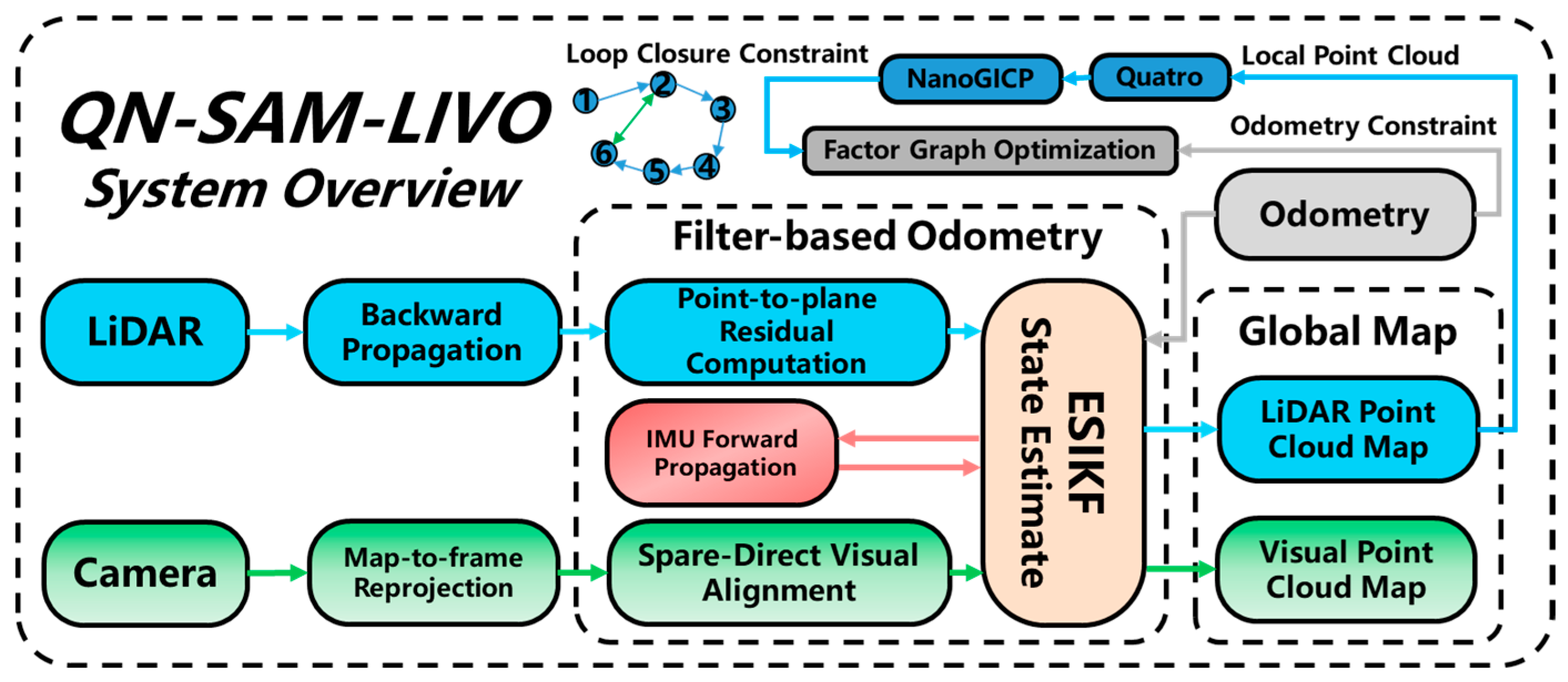
We present a real-time simultaneous localization, mapping, and coloring framework. Three parts of this framework are integrated through an ESIKF: the LIO module, the VIO module, and the loop closure detection module. The whole system fuses data from LIDAR, cameras, and IMUs together to achieve state estimation, while being able to reconstruct a dense, 3D, RGB-colored point cloud of the environment in real-time.
(2)
We propose a loop closure detection module utilizing Quatro and Nano-GICP, which accomplishes state estimation between LIDAR frames via a radius-based search and an extended point cloud alignment approach. Subsequently, we attain a more precise evaluation of the current state via factor graph optimization through the iSAM2 optimizer. The optimization framework exclusively contains the LIDAR odometry factor with the loop closure factor, resulting in a reduction in the optimization time for other states.
(3)
The developed system is validated on the open data sequence NTU VIRAL dataset [35] and our customized device data. The results show that our system outperforms other similar systems and that this approach effectively corrects the degradation of the LIO scheme in structured scenarios.
Abbreviations used in this paper have been compiled in a table in Abbreviations for better comprehension.

2. System Overview

An overview of our system is shown in Figure 1. It consists of three components: the LIO module, the VIO module, and the loop closure detection module, which estimate the states within the framework of the error state iterative Kalman filter, and together maintain the LIDAR global map and the visual global map, as described in Section 2.3.
The LIO module compensates for the motion distortion error of the LIDAR via back propagation based on the estimated state of the IMU, and finally obtains the odometry of the LIO module by constraining the residuals of the mapping from the point to the plane in the LIDAR frames. The VIO module uses LIDAR sparse measurements within the camera FOV through a non-feature-extracted direct matching method and tracks the image by minimizing the direct photometric error. To further improve the LIDAR measurements, we added a synchronously threaded, low-occupancy, optimization-based, coarse-to-fine loop closure detection module for correcting cumulative errors over long periods of time and distances, and updated the optimized localization information obtained from the QN-c2f-SAM module matching into a Kalman filter to obtain a more accurate state estimation, as described in Section 5. The three modules are tightly coupled together through an ESIKF, so that the IMU measurements performed with multiple sensors, image alignment based on photometric errors, and LIDAR scanning alignment together enable the acquisition of high-precision odometry, and are able to operate for long periods of time without cumulative systematic errors.

2.1. Filter-Based Odometry

2.1.1. System Definitions

In our system, we assume that the time offsets between the three sensors (LIDAR, the IMU, and the camera) are known and can be calibrated or synchronized in advance. We use the IMU coordinate system (denoted as I) as the body coordinate system, and the first-frame body coordinate system as the global coordinate system origin (denoted as G). In addition, we assume that the three sensors are rigidly connected together and that all external sensors used are pre-calibrated.

2.1.2. The Boxplus “ ” and Boxminus “ ” Operator

The equation of state used in this paper is defined with the specified manifold M = S O ( 3 ) × R n , and the two operators “ ” and “ ” are defined to carry out the computation of the state error with the manifold:
                                : M × R n M ;                                       : M × M R n M = S O ( 3 ) :       R r = R Exp ( r ) ;     R 1 R 2 = Log R 2 T R 1 M = R n :                   a b = a + b ;                   a b = a b
with r R 3 , a , b R n . E x p ( ) and L o g ( ) denote the bi-directional mappings between rotation matrices and rotation vectors derived from Rodrigues’s formula. Thus, we can obtain the following definition of the state operation equation:
R a r b = R r a + b , R 1 a R 2 b = R 1 R 2 a b

2.1.3. Discrete State Transition Model

Based on the operations defined in (1), we can obtain the following discrete state transfer model at the i th IMU measurement:
x i + 1 = x i ( Δ t f ( x i , u i , w i ) )
where Δ t is the IMU sample period, and the state x , input u , process noise w , and function f are defined as follows:
M = S O ( 3 ) × R 15 , d i m ( M ) = 18 x [ G R I T G p I T G v I T b ω T b a T G g T ] T M u [ ω m T a m T ] T , w [ n ω T n a T n b ω T n b a T ] T f ( x i , u i , w i ) = ω m i b ω i n ω i G v I i G R I i a m i b a i n a i + G g i n b ω i n b a i 0 3 × 1
where G R I and   G p I denote the current pose and position in the global frame; G g denotes the unknown gravity vector; ω m and a m are directly measured by the IMU, accompanied by their corresponding white noise; and b ω and b a of the state are IMU biases, which are modeled as random walks driven by Gaussian noise n b ω and n b a .

2.2. IMU Forward Propagation

In the tightly coupled system proposed in this paper, the error calculations of both direct measurement models are based on the state estimates obtained from the forward propagation of high-frequency IMUs. Also the arrival of data from the three important modules mentioned in this paper (LIO module, VIO module, and loop closure module) triggers the forward propagation process of the IMU. When the IMU input data u i arrives, the calculation procedure for the state and its covariance, assuming a zero process error in (3), is as follows:
x ^ i + 1 = x ^ i Δ t f x ^ i , u i , 0
P ^ i + 1 = F δ x ^ P ^ i F δ x ^ T + F w Q F w T F δ x ^ = δ x ^ i + 1 δ x ^ i δ x ^ i = 0 , w i = 0 , F w = δ x ^ i + 1 w i δ x ^ i = 0 , w i = 0
where Q is the covariance of w . The associated estimation error is propagated in the linearized error space as follows (more detailed derivations are available in Appendix A):
δ x ^ i + 1 = x i + 1 x ^ i + 1 = x i Δ t f x i , u i , w i x ^ i Δ t f x ^ i , u i , 0 N 0 , Σ δ x ^ k + 1 ,
where:
Σ δ x ^ i + 1 = F δ x ^ Σ δ x ^ i F δ x ^ T + F w Q F w T F δ x ^ = δ x ^ i + 1 δ x ^ i δ x ^ i = 0 , w i = 0 , F w = δ x ^ i + 1 w i δ x ^ i = 0 , w i = 0
The time for IMU forward propagation (Equations (5) and (6)) is the time between measurements of the two key data, i.e., from the time of arrival of the previous LIDAR or image, t i + 1 , to the time of arrival of the propagation to the current LIDAR or image data, t k . In general, forward propagation involves using the current state estimate obtained by the ESIKF as the base state, and the results are used to calculate the error terms required for the ESIKF. Particularly, when loop closure detection optimization yields superior results, the base state is replaced with the latest state obtained from the loop closure module.

2.3. Map Management

In this paper, map management encompasses three distinct types of point cloud maps: a LIDAR point cloud map designed for LIDAR point cloud matching, a point-patch cloud map utilized for photometric error calculation, and a colored point cloud map employed for visualization purposes.

2.3.1. LIDAR Point Cloud Map

LIDAR point clouds are organized and queried using the ikd-Tree method described in [22]. The merging of scan results of point clouds is triggered by the update rate of filters caused by the LIO module or loop closure module. The insertion of new map points occurs recursively under downsampling at a given resolution. To maintain efficient queries during prolonged operation, only points within a distance l from the current state position are involved in building the ikd-Tree. Additionally, during each incremental process, the ikd-Tree actively monitors its balance characteristics. It dynamically rebalances itself by reconstructing relevant subtrees, ensuring complete accuracy in nearest neighbor searches through its reconstruction mechanism with a caching mechanism.

2.3.2. Point-Patch Cloud Map

The point-patch cloud map utilized for the VIO module is fundamentally a sparse point cloud map jointly constructed by points from the LIDAR point cloud map and their observed patches. Its data structure encompasses voxel positions for swift indexing, patch pyramids for all images, observing the point along with their corresponding poses, and the specific location in the global coordinate system. When data points in the point-patch cloud map are employed for error computation in the VIO module, post-projection, a rejection mechanism using outlier removal, as outlined in the “livo” method, is applied to eliminate points with depth inconsistencies or those obscured in the image. Updates to points in the map occur when the distance exceeds a set value or when the computed photometric difference surpasses a defined range.

2.3.3. Colored Point Cloud Map

Traditional LIO systems typically visualize point clouds using intensity points or physical information such as position and height, making it challenging to intuitively assess the true attributes of objects. Although VIO systems can densely map and capture point clouds with genuine color information, their poor depth quality often leads to suboptimal mapping results.
In contrast, the multi-sensor SLAM system proposed in this paper goes beyond conventional approaches. It projects registered LIDAR point clouds onto corresponding frames of images, extracting RGB information from the images. This process results in a colored point cloud map that offers superior visualization compared to visually dense maps. In comparison to FAST-LIVO, this paper further optimizes the adaptation process for commonly used mechanical LIDARs, achieving a comprehensive RGB point cloud mapping visualization algorithm applicable to all prevalent types of LIDARs in the market.

2.4. Frame-to-Map Measurement Error Model

2.4.1. LIDAR Point-to-Plane Residual Error Model

During the measurement process of mechanical LIDAR, motion distortion can lead to a mismatch between the collected point cloud and the reference frame. Utilizing the reverse propagation method in [21], it is possible to compensate for the point cloud   L p j collected at sampling intervals in the local LIDAR coordinate system L at the time t k when a certain level of cumulative data is reached. Assuming these corrected point clouds are adjacent to a normal u j   and a central point q j in the global map, we can define the error term as these point-to-plane distances when the point cloud is projected into the global coordinate system:
r l x ˇ k + 1 , L p j = u j T G T I k + 1 I T L L p j q j

2.4.2. Visual Photometric Error

In processing visual data, this paper employs a sparse direct matching method based on [5] that does not rely on visual features. This approach omits the conventional VIO stages of visual feature extraction and depth estimation. Instead, it directly utilizes the visual intensity point cloud from camera-observed patches for the matching and tracking processes, yielding motion state estimation results between visual images, as schematically shown in Figure 2.
Precisely, we implement a relative transformation I k ( · ) from the global points   G p i in the visual point cloud map to the points corresponding to the current frame. By projecting these points using π ( · ) , we filter out those within the camera field of view (FOV) and match the newly obtained sparse image points with the nearest projected points. This process yields the observation paths Q i for the same point in other images and their corresponding coefficients A i for the photometric value retrieval. The visual error term, formulated for state updates, manifests as the photometric error resulting from distinct observation paths within the sparse point block obtained in the current image:
r c x ˇ k + 1 , G p i = I k + 1 π I T C 1 G T I k + 1 1 G p i A i Q i

2.4.3. Loop Closure Detection Error Model

The specific method for loop closure detection is detailed in Section 5. The foundational factor graph nodes are established based on the poses of each historical LIDAR keyframe, and initial pose transformations between nodes are obtained using the corresponding odometry differences at each moment. Newly received LIDAR keyframes are inserted as new nodes into the existing factor graph. They are matched with the closest keyframes based on odometry information using the minimum radius method. When an accurate loop closure is detected, the calculated pose transformation between the current keyframe and its corresponding loop closure frame serves as an edge. This edge, along with odometry transformation edges between other neighboring nodes, is used in conjunction with the Bayesian tree’s incremental smoothing and mapping to optimize the factor graph [19]. The results of graph optimization are then used to update the foundational state of the current system.

2.5. ESIKF Update

Building upon the forward propagation of IMU data conducted in (5) to obtain the state x k + 1 , with reference to the derivation in [34], we can define its prior distribution as follows:
x k + 1 x ^ k + 1 = x ˇ k + 1 δ x ˇ k + 1 x ^ k + 1 x ˇ k + 1 x ^ k + 1 + H δ x ˇ k + 1 N 0 , Σ δ x ^ k + 1
with
H = x ˇ k + 1 δ x ˇ k + 1 x ^ k + 1 δ x ˇ k + 1 δ x ˇ k + 1 = 0
Hence, the prior distribution of δ x ˇ k + 1 in Equation (7) can be articulated as follows:
δ x ˇ k + 1 N H 1 x ˇ k + 1 x ^ k + 1 , H 1 Σ δ x ^ k + 1 H T
Taking into account the measurement errors involved in the direct method, and combining it with the prior distribution in (13), we can obtain the maximum a posteriori (MAP) estimate for δ x ˇ k + 1 by cumulatively combining the error distributions from the LIDAR measurement and the image formula. The MAP estimate is expressed as follows:
m i n δ x ˇ k + 1   x ˇ k + 1 x ^ k + 1 + H δ x ˇ k + 1 Σ δ x ~ k + 1 1 + j = 1 m l   r l x ˇ k + 1 , L p j + H j l δ x ˇ k + 1 Σ α j 1 2 + s = 1 m c   r c x ˇ k + 1 , C p s , G P s + H s c δ x ˇ k + 1 Σ β s 1 2
where the cumulative formula is given by x Σ 2 = x T Σ 1 x , with other notations maintained as follows:
H T = H 1 l , , H m l l , H 1 c T , , H m c c T R = diag Σ α 1 , , Σ α m l , Σ β 1 , , Σ β m c z ˇ k + 1 T = r l x ˇ k + 1 , L p 1 , , r l x ˇ k + 1 , L p m l , r c x ˇ k + 1 , C p 1 , G P 1 , , r c x ˇ k + 1 , C p m c , G P m c P = ( H ) 1 Σ δ x ^ k + 1 ( H ) T
The update for the Kalman gain is referenced from [21]:
K = H T R 1 H + P 1 1 H T R 1
Finally, the updated state can be derived as follows:
x ˇ k + 1 = x ˇ k + 1 K z ˇ k + 1 ( I K H ) ( H ) 1 x ˇ k + 1 x ^ k + 1
In this context, optimization takes the form of the iterated Kalman filter using the Gauss–Newton method [30] for iterative solving. The optimized state, as indicated in Equations (16) and (17), is subsequently employed in the IMU forward propagation process outlined in Equations (5) and (6). Concurrently, the map management described in Section 2.3 also uses the updated state as the odometry for registration:
x ^ k + 1 = x ˇ k + 1 , Σ ^ δ x ¯ k + 1 = ( I K H ) Σ ˇ δ x k + 1
It is essential to emphasize that this formula can have different forms depending on the triggering of different modules within the system. For instance, when the results from the loop closure module arrive, the updated state values and error terms change from the filter’s updated results to the loop closure results. Similarly, for the two error terms, when LIDAR data arrives, the image photometric residual term will not be activated, and vice versa.

3. QN-C2F-SAM Loop Method

The tightly coupled framework established by FAST-LIVO [29] performs well in the realm of multi-sensor fusion, but it lacks an effective solution for errors accumulated over a long period. We propose QN-C2F-SAM, a coarse-to-fine point cloud loop closure method. This approach utilizes optimized odometry information and local point clouds. It employs the QN-C2F point cloud registration method to search for and obtain relative poses within a certain radius R for historical keyframes. Subsequently, an incremental factor graph is constructed, and the iSAM optimizer is employed to optimize the poses of historical keyframes, resulting in a more accurate transformation for the current pose. Its structure is depicted in Figure 3.

3.1. Coarse Matching Method

Quatro [36] is an efficient point cloud registration method operating at a global scale. It takes full advantage of the characteristics of small rotations in the x- and y-axis directions in urban spaces. Instead of the general rotation R ^ + , it employs an approximate estimation of rotation R ^ , which is more focused on the z-axis. This approach effectively addresses the issue of degraded matching quality due to large viewpoint distances and excessive rotations. It completes the task of estimating relative poses for loop closure candidates in various degenerate situations. We utilize the Quatro-SO(3) estimation algorithm and the COTE algorithm to estimate the transformation T , composed of the rotation relationship R ^ + and translation estimate t ^ , between the current keyframe point cloud and the historical keyframes within a radius r . We consider them as two matching point cloud clusters A = a i , B = b i .

3.2. Fine Matching Method

The standard ICP method [37] is renowned for its exceptional accuracy, but this algorithm (as well as other ICP variants) heavily relies on nearest neighbor searches to associate the closest points [38]. NanoFLANN, a derivative of FLANN, is a C++ library based on kd-Trees. It is designed to approximate the neighbors around a point in a two-dimensional or three-dimensional point cloud. It is invoked within the nearest neighbor function to expedite the computation speed of FeatureAffine and Strain. GICP [39], building upon the standard ICP algorithm, extends the matching approach by utilizing the surface covariance matrix of the point cloud to construct the cost function, as follows:
We use Gaussian distributions to define the previously matched point cloud clusters, where a i N a ^ i , C i A , b i N b ^ i , C i B is the covariance matrix for each corresponding point. We combine the estimates obtained from Quatro to define the rigid transformation matrix T . Thus, the matching error can be defined in the following form:
d ^ i = b ^ i T a ^ i
Due to the translational invariance property of the Gaussian distribution, the registration error in (18) can be expressed as:
d i N b ^ i T a ^ i , C i B + T C i A T T = N 0 , C i B + T C i A T T
Therefore, the cost function in the standard ICP process is replaced by:
T = arg m i n T i   d i T C i B + T C i A T T 1 d i
In the selection of the optimizer, we adhered to the choice of the Gauss–Newton optimizer used in VGICP [39]. This has been validated to demonstrate superior speed and accuracy compared to the Broyden–Fletcher–Goldfarb–Shanno (BFGS) optimizer in the PCL library.

3.3. Factor Graph Optimization

Concurrently, we utilize the optimized odometry information and local point cloud map information from the other two modules as inputs to construct an incremental graph. This graph has states as nodes, and frame-to-frame pose relations along with loop closure detections as factors. The update process of this graph is computationally lightweight: when only frame-to-frame pose relations are present as factors, the incremental graph will not trigger an optimization process. The iSAM2 optimizer [19] updates the entire graph only when the point cloud registration result is added as a loop closure factor to the graph.
In a filter-based reasoning SLAM system faced with inputs of lower quality, noticeable cumulative errors may occur. For our loop closure system, factor graph optimization is employed to store and build relationships among sparse historical keyframes. This enables us to eliminate accumulated errors resulting from degradation and misalignment by leveraging both loop closure constraints and inter-frame pose change constraints when a loop is detected.

4. Experiments and Results

In this section, we will validate the proposed method using both open and private datasets.

4.1. Benchmark Dataset

In this segment, quantitative experiments have been systematically conducted on the complete set of nine sequences encompassed within the NTU-VIRAL open dataset [35]. This dataset incorporates data from the left camera, the horizontal 16-channel OS1 gen14 Light Detection and Ranging (LIDAR) sensor, and its internal Inertial Measurement Unit (IMU). For these, we measured fundamental information such as time and distance, and the results are presented in Table 1.
The evaluative framework involves a comparative analysis of our proposed methodology against several open-source odometry systems, which include FAST-LIVO [29]—a tightly coupled LIDAR-inertial-visual odometry employing a direct method. Additionally, R2LIVE [34], characterized by feature-based full LIDAR-inertial-visual odometry, SVO2.0 [40], a semi-direct visual-inertial odometry, and DVL-SLAM [41], a direct LIDAR-visual SLAM system, are included in the comparative assessment. All systems were downloaded from their GitHub repositories. R2LIVE and DVL-SLAM used the recommended outdoor parameters. SVO2.0 parameters were tuned for optimal results. The control experiment used the same DVL-SLAM version as FAST-LIVO, maintaining sliding window optimization for accuracy. Our reason for not discussing the excellent multi-sensor solution LVI-SAM in this paper is that it requires a nine-axis IMU as a data input.

4.1.1. Algorithmic Analysis Tool

In this study, all algorithm-derived odometry data were stored in TUM format, and comparative experiments were conducted using the evo tool, which is a widely utilized toolkit for processing, evaluating, and comparing the trajectory outputs of odometry obtained through SLAM algorithms. The odometry and the ground truth of the dataset were initially filtered based on ROS timestamps under the TUM format. Subsequently, spatial registration was conducted using the Umeyama method [42], and evaluation metrics such as the absolute translational error (APE), relative translational error (RPE), and root mean squared error (RSME) over the entire time domain were employed to assess trajectory accuracy.

4.1.2. Numerical Comparison

The RMSE results of the APE obtained through evo across the entire sequence are presented in Table 2, with each method employing consistent parameters across all sequences. Our method demonstrated the superior accuracy in most sequences, except for the “sbs 02” and “sbs 03” sequences, where it only falls below FAST-LIVO. We attribute this to the challenges in the loop closure detection process, wherein rapid changes in the UAV’s orientation hindered the low-frequency loop module from obtaining sufficient positional information. Benefiting from the tight coupling of multi-sensor information, our approach outperforms traditional visual/LIDAR SLAM methods that rely solely on the IMU for auxiliary information.
Due to the inadequate prior information caused by the rapid rotation of the UAV and strong image blurring, SVO 2.0 fails in some sequences. In contrast, DVL-SLAM, utilizing LIDAR measurements in its VO module, survived in these sequences. R2LIVE, employing point cloud features for matching, encounters reduced data availability when a non-solid-state radar is used. FAST-LIVO, lacking a loop closure module, exhibits noticeable odometer accuracy deviations in long-duration, long-distance scenarios. However, excessive loop closure detection optimization in regions of minor UAV positional changes may lead to reduced accuracy.

4.1.3. Visual Comparison

The visualization trajectory tool in the evo toolkit offers a more intuitive and clear presentation of data comparison and error distribution among different algorithms. Figure 4 and Figure 5 illustrates the trajectory comparison distribution and independent deviations in the x, y, and z directions for FAST-LIVO, SVO 2.0, and our algorithm on sequences “eee_03” and “nya_01”. It is evident that our algorithm achieved the best results in both scenarios. During our analysis, we observed that FAST-LIVO and SVO, when subjected to time-matched filtering through evo, exhibited significantly fewer fundamental matching points compared to our approach. This discrepancy resulted in non-smooth trajectories in the figures. In comparison, while FAST-LIVO obtained results closer to the ground truth trajectory, it exhibited noticeable jitter in certain rotations in the “eee_03” sequence. In the “nya_01” sequence, characterized by a narrower overall range of motion, our algorithm maintained its accuracy, similar to FAST-LIVO.
In Figure 6, we present a comparative error distribution between our algorithm and FAST-LIVO. Error calculations were conducted by comparing the trajectories obtained by both algorithms with the ground truth trajectory in the “nya_03” sequence, utilizing various calculation methods for result analyses. The error distributions for both algorithms are similar in their APE values, with our algorithm slightly outperforming FAST-LIVO, particularly in trajectories near the edges. Regarding RPE distribution, our algorithm significantly outperforms FAST-LIVO, achieving errors below the median in the majority of trajectories.

4.2. Private Dataset

4.2.1. Handheld Device Dataset

Our data acquisition setup, illustrated in Figure 7, comprises a VLP-16 LIDAR(Velodyne, San Jose, Silicon Valley, CA, USA), an D455 camera (Intel, Santa Clara, CA, USA), and a MicroStrain 3DM-GX5-25 IMU(Parker Hannifin, Cleveland, OH, USA). These devices can be affixed to a compact vehicle platform through connectors or operated manually. The sensors, characterized by distinct frequencies, undergo time-soft synchronization via ports in a Precision Time Protocol (PTP) mode, ensuring uniform timestamps within the Robot Operating System (ROS) framework.
In the delineated dataset, the entire data collection process was conducted by an operator holding the device. The scenes encompass a wide range of dynamic objects, structural and non-structural point clouds, as well as variations in brightness within small tunnels. Figure 8 illustrates the trajectory schematic and angular velocity changes. For testing the loop closure module, the recorded routes include identifiable similar scenes in both forward and reverse directions. Unlike scenarios involving vehicles or UAVs, the system’s motion process is slower, introducing numerous small disturbances caused by shaking and oscillations, amplifying measurement noise in the IMU. The dataset also includes significant variations in lighting conditions, transformations between structured and unstructured environments, and some dynamic interferences, including moving crowds and nearby cycling motion. Overall, this presents a relatively challenging scenario for comprehensive assessment.
The camera–IMU calibration was accomplished by determining the extrinsic parameters through the stereo version of VINS-FUSION. The resultant obtained parameters between the IMU and the left camera were utilized for calibration. For the LIDAR–IMU calibration, the online calibration method from FAST-LIO2 [22] was employed, optimizing the calibration in standard structured scenes.

4.2.2. Mapping with Normal Point Cloud

Our proposed method successfully generated highly detailed point cloud maps on a private dataset. The projection of the results onto real satellite images are illustrated in Figure 9. Particularly when viewed from a top angle, the mapping performance is outstanding, showcasing detailed representations of buildings and roads. There is no noticeable z-axis offset in the planar view. When observed from a third perspective, the point cloud maps exhibit a high level of fidelity with no evident trailing or noise issues.
We compared the results obtained in this study with some exemplary radar-based SLAM solutions, and the outcomes of this comparison are presented in Figure 10. Initially, the performance of FAST-LIO2 exhibited a commendable mapping quality in the early stages, but experienced degradation when navigating through a challenging narrow tunnel, resulting in a decline in the initially high-precision mapping performance. Both LIO-SAM and our proposed method produced point cloud maps with comparable effects; however, our algorithm demonstrated superior accuracy at specific locations, such as road and building boundaries, manifesting a slight overall angular offset. In the case of LVI-SAM, utilizing identical sensor extrinsics, the system failed to successfully complete the mapping task, experiencing degradation within the initial 20 s of the dataset and leading to irreversible drift (whether employing real-time extrinsic optimization or fixed extrinsics).
In the context of point cloud details, we conducted an exhaustive comparative analysis between our algorithm and FAST-LIO2 across various categories of point cloud details, as elucidated in Figure 11. In Figure 11a,b, depicting structured scenes at the edges and center, our algorithm captures detailed features, while FAST-LIO2 exhibits incorrect artifacts due to rotational scale drift, particularly evident around the depicted vehicle. Figure 11c highlights clearer boundaries in our algorithm with fewer point clouds, despite noise introduced by dynamic objects. Nonetheless, the presence of dynamic elements such as people and bicycles introduces some noise points, particularly noticeable around the image center. In Figure 11d, the central display highlights the point cloud corresponding to the canopy of a tree within the scene. A comparative assessment underscores that our algorithm’s point cloud map distinctly delineates the boundaries between the tree trunk and the canopy. Even from a top view, the discernibility of the tree and surrounding structures is evident.

4.2.3. Mapping with RGB Point Cloud

The color point cloud mapping scheme proposed in FAST-LIVO is specifically designed for AVIA solid-state LIDAR and does not have compatibility with traditional mechanical LIDAR in a multi-sensor setup. This paper extends that groundwork and refines this approach, rectifying the inaccurate point cloud mapping relationships for mechanical LIDAR. The outcome is a mapping relationship aligned with the camera’s field of view (FOV), facilitating the generation of an RGB point cloud map.
The real-time reconstructed RGB point cloud map using our algorithm is illustrated in Figure 12. In comparison to conventional point cloud maps, color-coded based on intensity or position, the colored point cloud distinctly emphasizes object boundaries, thereby enhancing scene fidelity and improving the interpretability of the mapping process.

4.3. Time Analysis

In this section, we evaluated module time consumption on our eight-core Intel Core i7-10875 notebook PC, as shown in Table 3. The LIO module processed frames at the fastest rate, averaging at 18.02 ms. While the VIO module initially matched this rate, it stabilized at around three times the LIO module’s consumption as the map size increased. The loop closure module, based on optimization, followed a similar trend to the VIO module. By employing a faster point cloud matching tool and optimizing execution timing, the graph optimization per frame was reduced to 25.24 ms, resulting in an overall time consumption of 39.80 ms. It is evident that, by employing a faster point cloud matching tool and a low-frequency graph optimization design, we achieved real-time loop closure estimation with only a modest increase in time consumption.

5. Conclusions

This paper presents a fast, robust, sparse direct LIDAR-inertial-visual fusion framework, surpassing the state-of-the-art LIVO algorithm. We integrate LIDAR, inertial, and camera sensor measurements into an error-state iterative Kalman filter. The real-time loop closure module provides accuracy corrections for temporally and spatially repetitive scenes. When tested on open datasets, the experimental results showcase superior overall performance and robustness compared to advanced LIO, VIO, and LIVO algorithms. On private datasets, our system yields improved RGB point cloud mapping results with non-solid-state LIDAR.

Author Contributions

Conceptualization, W.W.; methodology, C.Y. and H.X.; software, Z.C. and H.X.; writing—original draft preparation, C.Y.; writing—review and editing, Y.H. and H.X.; supervision, W.W. All authors have read and agreed to the published version of the manuscript.

Funding

This research was funded by the National Key R&D Program of China (grant no. 2021YFC3100705), the Key Laboratory of Thermal Management and Energy Utilization of Aircraft, Ministry of Industry and Information Technology (grant no. CEPE2022016), and the State Key Laboratory of Mechanics and Control for Aerospace Structures (Nanjing University of Aeronautics and Astronautics) (grant no. MCMS-E-0323Y01).

Data Availability Statement

The open-source data presented in this study are openly available at https://ntu-aris.github.io/ntu_viral_dataset/ (accessed on 6 November 2021) and at https://doi.org/10.1177/02783649211052312 (accessed on 6 November 2021), reference number [35]. The data presented in this study are available on request from the corresponding author. The private data are not publicly available due to some sensitive scenarios involved in the dataset.

Conflicts of Interest

The authors declare no conflict of interest.

Abbreviations

SLAMSimultaneous Localization and Mapping
LIDARLight Detection and Ranging
IMUInertial Measurement Unit
ICPIterative Closest Point
LOAMLIDAR Odometry and Mapping
VIOVisual-Inertial Odometry
LIOLIDAR-Inertial Odometry
LVIOLIDAR-Visual-Inertial Odometry
ESIKFError-State Iterative Kalman Filter
UAVUnmanned Aerial Vehicles
APEAbsolute Pose Error
RPERelative Pose Error

Appendix A

Initially, within the ESIKF framework, the error terms are depicted by the state estimates x i and their covariance Σ δ x ^ i in the tangent space as follows:
δ x ^ i x i x ^ i = G δ r ^ I i T G δ p ^ I i T I δ r ^ C i T I δ p ^ C i T G δ v ^ i T δ b ^ g i T δ b ^ a i T T N 0 21 × 1 , Σ δ x ^ i
with
  G δ r ^ I i = l o g   G R ^ I i T   G R I i T ,   I δ r ^ C i = l o g   I R ^ C i T   I R C i
Building upon Equations (3) and (5), we can extend Equation (7) to the following:
δ x ^ i + 1 = x i + 1 x ^ i + 1 = x i Δ t f x i , u i , w i x ^ i Δ t f x ^ i , u i , 0 = l o g   G R ^ I i E x p ω ^ i Δ t T   G R ^ I i E x p   G δ r I i E x p ω i Δ t   G δ p I i +   G δ v i Δ t + 1 2 a i Δ t 2 1 2 a ^ i Δ t 2   I δ r C i   I δ p C i   G δ v i +   G R ^ I i E x p   G δ r I i a i Δ t   G R ^ I i a ^ i Δ t δ b ω i + n b ω i δ b a i + n b a i N 0 , Σ δ x ^ i + 1
The following approximations of perturbation are employed to streamline the representation of error terms:
E x p ( r + δ r ) & E x p ( r ) E x p J r ( r ) δ r
E x p ( r ) E x p ( δ r ) & E x p r + J r 1 ( r ) δ r
R E x p ( δ r ) u & R I + [ δ r ] × u = R u R [ u ] × δ r
so that we have the following three simplifications for the representation.
log   G R ^ I i E x p ω ^ i Δ t T   G R ^ I i E x p   G δ r I i E x p ω i Δ t = log E x p ω ^ i Δ t T E x p   G δ r I i E x p ω i Δ t log E x p ω ^ i Δ t T E x p   G δ r I i E x p ω ^ i Δ t . Exp J r ω ^ i Δ t δ b ω i + n b ω i
Exp J r ω ^ i Δ t δ b g i + n g i Exp ω ^ i Δ t   G δ r I i J r ω ^ i Δ t T δ b g i J r ω ^ i Δ t T n b ω i
  G R I i E x p   G δ r I i a i Δ t   G R I i I +   G δ r I i × a ^ i δ b a i n b a Δ t G R I i a ^ i Δ t   G R I i δ b a i Δ t   G R I i n b a i Δ t   G R I i a ^ i ×   G δ r I i
Hence, we can derive a more intricate expression for F δ x ^ and F w in Equation (8), as follows:
F δ x ^ = δ x ^ i + 1 δ x ^ i δ x ^ i = 0 , w i = 0 = E x p ω ^ i Δ t 0 0 0 0 J r ω ^ i Δ t T 0 0 I 0 0 I Δ t 0 0 0 0 I 0 0 0 0 0 0 0 I 0 0 0 G R ^ I i a ^ i × Δ t 0 0 0 I 0 G R ^ I i Δ t 0 0 0 0 0 I 0 0 0 0 0 0 0 I
F w = δ x ^ i + 1 w i δ x ^ i = 0 , w i = 0 = J r ω ^ i Δ t T 0 0 0 0 0 0 0 0 0 0 0 0 0 0 0 0   G R ^ I i Δ t 0 0 0 0 I Δ t 0 0 0 0 I Δ t

References

  1. Cadena, C.; Carlone, L.; Carrillo, H.; Latif, Y.; Scaramuzza, D.; Neira, J.; Reid, I.; Leonard, J.J. Past, Present, and Future of Simultaneous Localization and Mapping: Toward the Robust-Perception Age. IEEE Trans. Robot. 2016, 32, 1309–1332. [Google Scholar] [CrossRef]
  2. Zhang, J.; Singh, S. LOAM: LIDAR Odometry and Mapping in Real-Time, Robotics: Science and Systems. In Proceedings of the Robotics: Science and Systems, Berkeley, CA, USA, 12–16 July 2014; Volume 2, pp. 1–9. [Google Scholar]
  3. Low, K.-L. Linear Least-Squares Optimization for Point-to-Plane ICP Surface Registration; University of North Carolina: Chapel Hill, NC, USA, 2004; pp. 2–4. [Google Scholar]
  4. Shan, T.; Englot, B. LeGO-LOAM: Lightweight and Ground-Optimized LIDAR Odometry and Mapping on Variable Terrain. In Proceedings of the 2018 IEEE/RSJ International Conference on Intelligent Robots and Systems (IROS), Madrid, Spain, 1–5 October 2018; pp. 4758–4765. [Google Scholar] [CrossRef]
  5. Chen, K.; Lopez, B.T.; Agha-Mohammadi, A.A.; Mehta, A. Direct LIDAR Odometry: Fast Localization With Dense Point Clouds. IEEE Robot. Autom. Lett. 2022, 7, 2000–2007. [Google Scholar] [CrossRef]
  6. Qin, T.; Li, P.; Shen, S. VINS-Mono: A Robust and Versatile Monocular Visual-Inertial State Estimator. IEEE Trans. Robot. 2018, 34, 1004–1020. [Google Scholar] [CrossRef]
  7. Mur-Artal, R.; Tardos, J.D. ORB-SLAM2: An Open-Source SLAM System for Monocular, Stereo, and RGB-D Cameras. IEEE Trans. Robot. 2017, 33, 1255–1262. [Google Scholar] [CrossRef]
  8. Campos, C.; Elvira, R.; Rodriguez, J.J.G.; Montiel, J.M.M.; Tardos, J.D. ORB-SLAM3: An Accurate Open-Source Library for Visual, Visual-Inertial, and Multimap SLAM. IEEE Trans. Robot. 2021, 37, 1874–1890. [Google Scholar] [CrossRef]
  9. Zhang, J.; Singh, S. Visual-LIDAR Odometry and Mapping: Low-Drift, Robust, and Fast. In Proceedings of the 2015 IEEE International Conference on Robotics and Automation (ICRA), Seattle, WA, USA, 26–30 May 2015. [Google Scholar] [CrossRef]
  10. Zhang, J.; Singh, S. Laser–Visual–Inertial Odometry and Mapping with High Robustness and Low Drift. J. Field Robot. 2018, 35, 1242–1264. [Google Scholar] [CrossRef]
  11. Wang, Z.; Zhang, J.; Chen, S.; Yuan, C.; Zhang, J.; Zhang, J. Robust High Accuracy Visual-Inertial-Laser SLAM System. In Proceedings of the 2019 IEEE/RSJ International Conference on Intelligent Robots and Systems (IROS), Macau, China, 3–8 November 2019; pp. 6636–6641. [Google Scholar] [CrossRef]
  12. Lowe, T.; Kim, S.; Cox, M. Complementary Perception for Handheld SLAM. IEEE Robot. Autom. Lett. 2018, 3, 1104–1111. [Google Scholar] [CrossRef]
  13. Forster, C.; Carlone, L.; Dellaert, F.; Scaramuzza, D. IMU Preintegration on Manifold for Efficient Visual-Inertial Maximum-a-Posteriori Estimation. In Proceedings of the Robotics: Science and Systems, Rome, Italy, 13–17 July 2015; Volume 11. [Google Scholar] [CrossRef]
  14. Forster, C.; Carlone, L.; Dellaert, F.; Scaramuzza, D. On-Manifold Preintegration for Real-Time Visual--Inertial Odometry. IEEE Trans. Robot. 2017, 33, 1–21. [Google Scholar] [CrossRef]
  15. Geneva, P.; Eckenhoff, K.; Yang, Y.; Huang, G. LIPS: LIDAR-Inertial 3D Plane SLAM. In Proceedings of the 2018 IEEE/RSJ International Conference on Intelligent Robots and Systems (IROS), Madrid, Spain, 1–5 October 2018; pp. 123–130. [Google Scholar] [CrossRef]
  16. Gentil, C.L.; Vidal-Calleja, T.; Huang, S. IN2LAMA: INertial LIDAR Localisation And MApping. In Proceedings of the 2019 International Conference on Robotics and Automation (ICRA), Montreal, QC, Canada, 20–24 May 2019; pp. 6388–6394. [Google Scholar] [CrossRef]
  17. Ye, H.; Chen, Y.; Liu, M. Tightly Coupled 3D LIDAR Inertial Odometry and Mapping. In Proceedings of the 2019 International Conference on Robotics and Automation (ICRA), Montreal, QC, Canada, 20–24 May 2019. [Google Scholar] [CrossRef]
  18. Shan, T.; Englot, B.; Meyers, D.; Wang, W.; Ratti, C.; Rus, D. LIO-SAM: Tightly-Coupled LIDAR Inertial Odometry via Smoothing and Mapping. In Proceedings of the IEEE/RSJ International Conference on Intelligent Robots and Systems (IROS), Las Vegas, NV, USA, 24–30 October 2020. [Google Scholar] [CrossRef]
  19. Kaess, M.; Johannsson, H.; Roberts, R.; Ila, V.; Leonard, J.J.; Dellaert, F. ISAM2: Incremental Smoothing and Mapping Using the Bayes Tree. Int. J. Robot. Res. 2012, 31, 216–235. [Google Scholar] [CrossRef]
  20. Qin, C.; Ye, H.; Pranata, C.E.; Han, J.; Zhang, S.; Liu, M. LINS: A LIDAR-Inertial State Estimator for Robust and Efficient Navigation. In Proceedings of the 2020 IEEE International Conference on Robotics and Automation (ICRA), Paris, France, 31 May–31 August 2020. [Google Scholar] [CrossRef]
  21. Xu, W.; Zhang, F. FAST-LIO: A Fast, Robust LIDAR-Inertial Odometry Package by Tightly-Coupled Iterated Kalman Filter. IEEE Robot. Autom. Lett. 2021, 6, 3317–3324. [Google Scholar] [CrossRef]
  22. Xu, W.; Cai, Y.; He, D.; Lin, J.; Zhang, F. FAST-LIO2: Fast Direct LIDAR-Inertial Odometry. IEEE Trans. Robot. 2022, 38, 2053–2073. [Google Scholar] [CrossRef]
  23. Wang, T.; Su, Y.; Shao, S.; Yao, C.; Wang, Z. GR-Fusion: Multi-Sensor Fusion SLAM for Ground Robots with High Robustness and Low Drift. In Proceedings of the 2021 IEEE/RSJ International Conference on Intelligent Robots and Systems (IROS), Prague, Czech Republic, 27 September–1 October 2021; pp. 5440–5447. [Google Scholar] [CrossRef]
  24. Jia, Y.; Luo, H.; Zhao, F.; Jiang, G.; Li, Y.; Yan, J.; Jiang, Z.; Wang, Z. Lvio-Fusion: A Self-Adaptive Multi-Sensor Fusion SLAM Framework Using Actor-Critic Method. In Proceedings of the 2021 IEEE/RSJ International Conference on Intelligent Robots and Systems (IROS), Prague, Czech Republic, 27 September–1 October 2021; pp. 286–293. [Google Scholar] [CrossRef]
  25. Zheng, T.X.; Huang, S.; Li, Y.F.; Feng, M.C. Key Techniques for Vision Based 3D Reconstruction: A Review. Zidonghua Xuebao/Acta Autom. Sin. 2020, 46, 631–652. [Google Scholar] [CrossRef]
  26. Theodorou, C.; Velisavljevic, V.; Dyo, V. Visual SLAM for Dynamic Environments Based on Object Detection and Optical Flow for Dynamic Object Removal. Sensors 2022, 22, 7553. [Google Scholar] [CrossRef]
  27. Shan, T.; Englot, B.; Ratti, C.; Rus, D. LVI-SAM: Tightly-Coupled LIDAR-Visual-Inertial Odometry via Smoothing and Mapping. In Proceedings of the 2021 IEEE International Conference on Robotics and Automation (ICRA), Xi’an, China, 30 May–5 June 2021. [Google Scholar] [CrossRef]
  28. Yang, Y.; Geneva, P.; Zuo, X.; Eckenhoff, K.; Liu, Y.; Huang, G. Tightly-Coupled Aided Inertial Navigation with Point and Plane Features. In Proceedings of the 2019 International Conference on Robotics and Automation (ICRA), Montreal, QC, Canada, 20–24 May 2019; pp. 6094–6100. [Google Scholar] [CrossRef]
  29. Zheng, C.; Zhu, Q.; Xu, W.; Liu, X.; Guo, Q.; Zhang, F. FAST-LIVO: Fast and Tightly-Coupled Sparse-Direct LIDAR-Inertial-Visual Odometry. In Proceedings of the 2022 IEEE/RSJ International Conference on Intelligent Robots and Systems (IROS), Kyoto, Japan, 23–27 October 2022; pp. 4003–4009. [Google Scholar] [CrossRef]
  30. Bell, B.M.; Cathey, F.W. The Iterated Kalman Filter Update as a Gauss-Newton Method. IEEE Trans. Autom. Control 1993, 38, 294–297. [Google Scholar] [CrossRef]
  31. He, D.; Xu, W.; Zhang, F. Kalman Filters on Differentiable Manifolds. arXiv 2021, arXiv:2102.03804. [Google Scholar] [CrossRef]
  32. Zuo, X.; Geneva, P.; Lee, W.; Liu, Y.; Huang, G. LIC-Fusion: LIDAR-Inertial-Camera Odometry. In Proceedings of the IEEE International Conference on Intelligent Robots and Systems, Macau, China, 3–8 November 2019. [Google Scholar] [CrossRef]
  33. Zuo, X.; Yang, Y.; Geneva, P.; Lv, J.; Liu, Y.; Huang, G.; Pollefeys, M. LIC-Fusion 2.0: LIDAR-Inertial-Camera Odometry with Sliding-Window Plane-Feature Tracking. In Proceedings of the IEEE International Conference on Intelligent Robots and Systems, Las Vegas, NV, USA, 24 October 2020–24 January 2021. [Google Scholar] [CrossRef]
  34. Lin, J.; Zheng, C.; Xu, W.; Zhang, F. R2LIVE: A Robust, Real-Time, LIDAR-Inertial-Visual Tightly-Coupled State Estimator and Mapping. IEEE Robot. Autom. Lett. 2021, 6, 7469–7476. [Google Scholar] [CrossRef]
  35. Nguyen, T.-M.; Yuan, S.; Cao, M.; Lyu, Y.; Nguyen, T.H.; Xie, L. NTU VIRAL: A Visual-Inertial-Ranging-LIDAR Dataset, from an Aerial Vehicle Viewpoint. Int. J. Robot. Res. 2021, 41, 270–280. [Google Scholar] [CrossRef]
  36. Lim, H.; Yeon, S.; Ryu, S.; Lee, Y.; Kim, Y.; Yun, J.; Jung, E.; Lee, D.; Myung, H. A Single Correspondence Is Enough: Robust Global Registration to Avoid Degeneracy in Urban Environments. In Proceedings of the 2022 International Conference on Robotics and Automation (ICRA), Philadelphia, PA, USA, 23–27 May 2022; pp. 8010–8017. [Google Scholar] [CrossRef]
  37. Magnusson, M.; Lilienthal, A.; Duckett, T. Scan Registration for Autonomous Mining Vehicles Using 3D-NDT. J. Field Robot. 2007, 24, 803–827. [Google Scholar] [CrossRef]
  38. Rusinkiewicz, S.; Levoy, M. Efficient Variants of the ICP Algorithm. In Proceedings of the Third International Conference on 3-D Digital Imaging and Modeling, Quebec City, QC, Canada, 28 May–1 June 2001. [Google Scholar] [CrossRef]
  39. Koide, K.; Yokozuka, M.; Oishi, S.; Banno, A. Voxelized GICP for Fast and Accurate 3D Point Cloud Registration. In Proceedings of the 2021 IEEE International Conference on Robotics and Automation (ICRA), Xi’an, China, 30 May–5 June 2021; pp. 11054–11059. [Google Scholar] [CrossRef]
  40. Forster, C.; Zhang, Z.; Gassner, M.; Werlberger, M.; Scaramuzza, D. SVO: Semidirect Visual Odometry for Monocular and Multicamera Systems. IEEE Trans. Robot. 2017, 33, 249–265. [Google Scholar] [CrossRef]
  41. Shin, Y.S.; Park, Y.S.; Kim, A. DVL-SLAM: Sparse Depth Enhanced Direct Visual-LIDAR SLAM. Auton. Robot. 2020, 44, 115–130. [Google Scholar] [CrossRef]
  42. Umeyama, S. Least-Squares Estimation of Transformation Parameters Between Two Point Patterns. IEEE Trans. Pattern Anal. Mach. Intell. 1991, 13, 376–380. [Google Scholar] [CrossRef]
Figure 1. The overview of our proposed system.
Robotics 13 00002 g001
Figure 2. Our VIO module tracks with minimizing the frame-to-map photometric error of the patches under different states and different observation paths.
Robotics 13 00002 g002
Figure 3. Our loop detection module updates the state estimation by optimizing (with iSAM2) a factor graph based on both LIDAR odometry constraints and loop closure constraints.
Robotics 13 00002 g003
Figure 4. The left graph (a) illustrates distinct trajectories in the “eee_03” sequences, while the right graphs (b) display independent errors along the three axes.
Robotics 13 00002 g004
Figure 5. The left graph (a) illustrates distinct trajectories in the “nya_01” sequences, while the right graphs (b) display independent errors along the three axes.
Robotics 13 00002 g005
Figure 6. Error distribution along the trajectory, depicting (a) our method (APE), (b) FAST-LIVO (APE), (c) our method (RPE), and (d) FAST-LIVO (RPE).
Robotics 13 00002 g006
Figure 7. Our platform setup with software synchronization for data collection. (a) Composition of our hardware components, (b) schematic diagram of software time synchronization based on PTP.
Robotics 13 00002 g007
Figure 8. The upper panel illustrates a trajectory schematic of our proprietary dataset, while the lower panel depicts the corresponding gyroscope-measured angular velocity over time.
Robotics 13 00002 g008
Figure 9. Visualization of our point cloud mapping results. (a) Merged intensity-colored map and real satellite imagery; (b) buildings from a top view perspective; (c) roads and trees from a third-person perspective; (d) front view of the scene. The white boxes on the map show a narrow tunnel scene and some scenes with dynamic objects including pedestrians and bicycles.
Robotics 13 00002 g009
Figure 10. (a) The 3D mapping results of our method, FAST-LIO2 (b), LIO-SAM (c), and LVI-SAM (d) mapped onto our dataset. The point clouds are colored based on intensity.
Robotics 13 00002 g010
Figure 11. Detailed comparison of the intensity-colored point clouds generated by our algorithm and FAST-LIO2 mapped onto our proprietary dataset.
Robotics 13 00002 g011
Figure 12. Illustration of RGB-colored point cloud maps based on non-solid-state LIDAR. (a) Original incorrect projection method in FAST-LIVO. (b) Corrected projection method after our modification. (c) Comparison between intensity-colored and RGB-colored point clouds, the red box shows the real picture, and the white box shows the corresponding point cloud details.
Robotics 13 00002 g012
Table 1. Details of all benchmark datasets.
NameDistance (m)Duration (s)Remark
eee_01237.01 m398.7 sCollected at the School of EEE’s central carpark
eee_02171.08 m321.1 sCollected at the School of EEE’s central carpark
eee_03127.83 m181.4 sCollected at the School of EEE’s central carpark
sbs_01202.87 m354.2 sCollected at the School of Bio. Science’s front square
sbs_02183.57 m373.3 sCollected at the School of Bio. Science’s front square
sbs_03198.54 m389.3 sCollected at the School of Bio. Science’s front square
nya_01160.24 m396.3 sCollected inside the Nanyang Auditorium
nya_02249.10 m428.7 sCollected inside the Nanyang Auditorium
nya_03315.47 m411.2 sCollected inside the Nanyang Auditorium
Table 2. Absolute translational errors (RMSE, METERS) in NTU-VIRAL datasets with good ground truth.
eee_01eee_02eee_03sbs_01sbs_02sbs_03nya_01nya_02nya_03
Ours0.220.200.250.250.240.220.230.230.25
FAST-LIVO0.240.270.270.240.230.30.240.250.28
R2LIVE0.620.440.970.670.310.480.310.630.31
SVO2.0FailFail5.258.88FailFail2.493.564.49
DVL-SLAM2.962.565.222.042.582.553.582.343.33
Table 3. Mean time consumption of different process steps in military seconds.
LIO ModuleVIO ModuleLoop Closure Module
QuatroGICPGraph Optimization
(Average per Frame)
Total Time
Intel i7-1087556.4618.021.0813.4825.2439.80
Disclaimer/Publisher’s Note: The statements, opinions and data contained in all publications are solely those of the individual author(s) and contributor(s) and not of MDPI and/or the editor(s). MDPI and/or the editor(s) disclaim responsibility for any injury to people or property resulting from any ideas, methods, instructions or products referred to in the content.

