
A Novel Control Architecture Based on Behavior Trees for an Omni-Directional Mobile Robot


Abstract
:1. Introduction
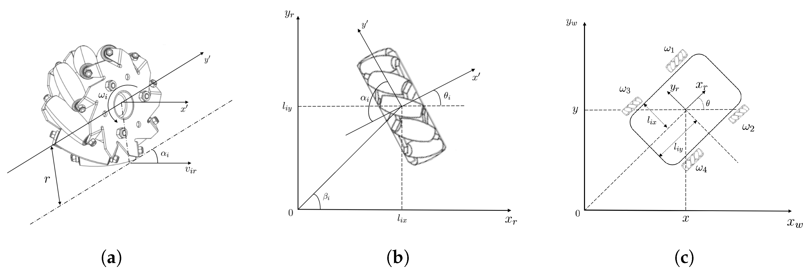
2. Robot Modeling
Kinematics Modeling
3. Proposed Control Architecture
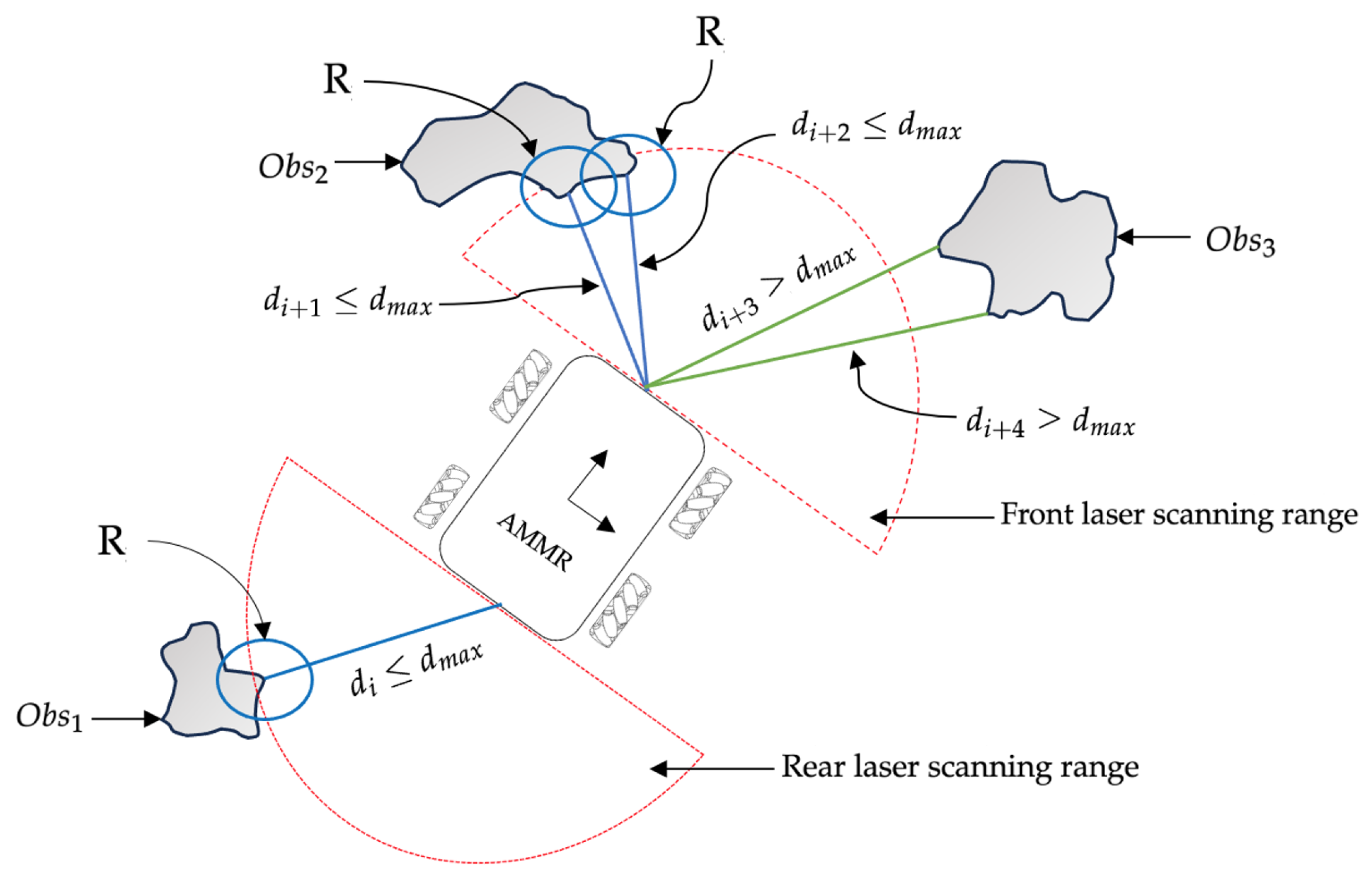
3.1. Detection of Obstacles for Collision Avoidance
3.1.1. Autonomous Obstacle Detection
3.1.2. Previously Known Obstacles
3.2. Controller Formulation
3.3. NMPC Implementation
3.4. Implementation in the ROS Environment
4. Simulation and Experimental Results
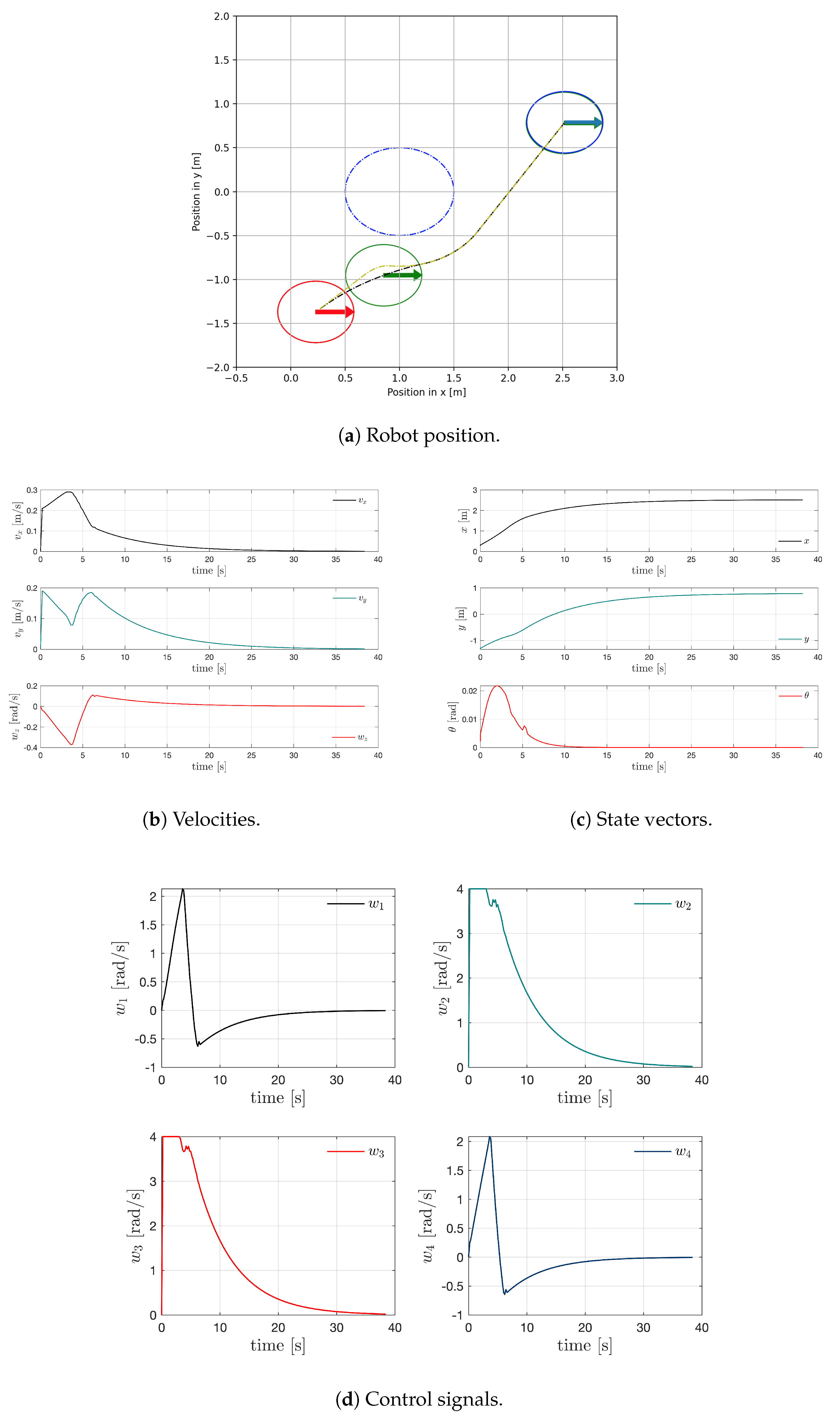
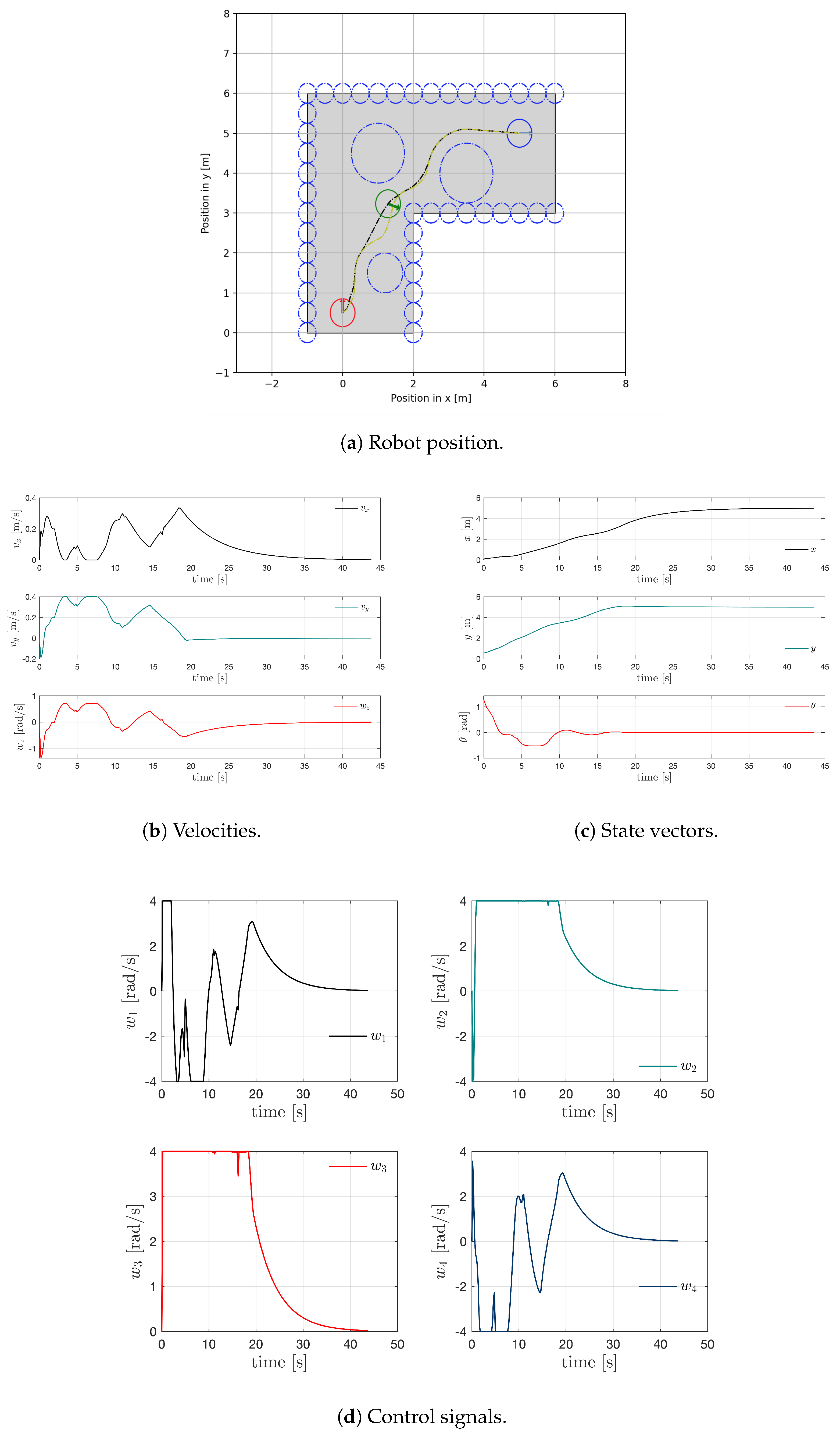
4.1. Simulation Results
4.2. Experimental Validation
5. Conclusions
Author Contributions
Funding
Data Availability Statement
Conflicts of Interest
References
- Bernardo, R.; Sousa, J.M.; Gonçalves, P.J. Survey on robotic systems for internal logistics. J. Manuf. Syst. 2022, 65, 339–350. [Google Scholar] [CrossRef]
- Elbanhawi, M.; Simic, M. Sampling-based robot motion planning: A review. IEEE Access 2014, 2, 56–77. [Google Scholar] [CrossRef]
- Zhang, J.; Shao, X.; Zhang, W.; Na, J. Path-Following Control Capable of Reinforcing Transient Performances for Networked Mobile Robots Over a Single Curve. IEEE Trans. Instrum. Meas. 2023, 72, 1–12. [Google Scholar] [CrossRef]
- Hung, N.; Rego, F.; Quintas, J.; Cruz, J.; Jacinto, M.; Souto, D.; Potes, A.; Sebastiao, L.; Pascoal, A. A review of path following control strategies for autonomous robotic vehicles: Theory, simulations, and experiments. J. Field Robot. 2023, 40, 747–779. [Google Scholar] [CrossRef]
- Gu, D.; Hu, H. Receding horizon tracking control of wheeled mobile robots. IEEE Trans. Control Syst. Technol. 2006, 14, 743–749. [Google Scholar]
- Ye, H.; Wang, S. Trajectory tracking control for nonholonomic wheeled mobile robots with external disturbances and parameter uncertainties. Int. J. Control. Autom. Syst. 2020, 18, 3015–3022. [Google Scholar] [CrossRef]
- Azizi, M.R.; Keighobadi, J. Point stabilization of nonholonomic spherical mobile robot using nonlinear model predictive control. Robot. Auton. Syst. 2017, 98, 347–359. [Google Scholar] [CrossRef]
- Rösmann, C.; Makarow, A.; Bertram, T. Online motion planning based on nonlinear model predictive control with non-euclidean rotation groups. In Proceedings of the 2021 European Control Conference (ECC), Delft, The Netherlands, 29 June–2 July 2021; pp. 1583–1590. [Google Scholar]
- Zavala, V.M.; Biegler, L.T. The advanced-step NMPC controller: Optimality, stability and robustness. Automatica 2009, 45, 86–93. [Google Scholar] [CrossRef]
- Mehrez, M.W.; Mann, G.K.; Gosine, R.G. Stabilizing nmpc of wheeled mobile robots using open-source real-time software. In Proceedings of the 2013 16th International Conference on Advanced Robotics (ICAR), Montevideo, Uruguay, 25–29 November 2013; pp. 1–6. [Google Scholar]
- Siegwart, R.; Nourbakhsh, I.R.; Scaramuzza, D. Introduction to Autonomous Mobile Robots; MIT Press: Cambridge, MA, USA, 2011. [Google Scholar]
- Rojas, R.; Förster, A.G. Holonomic control of a robot with an omnidirectional drive. KI-Künstliche Intell. 2006, 20, 12–17. [Google Scholar]
- Masmoudi, M.S.; Krichen, N.; Masmoudi, M.; Derbel, N. Fuzzy logic controllers design for omnidirectional mobile robot navigation. Appl. Soft Comput. 2016, 49, 901–919. [Google Scholar] [CrossRef]
- Zijie, N.; Qiang, L.; Yonjie, C.; Zhijun, S. Fuzzy control strategy for course correction of omnidirectional mobile robot. Int. J. Control Autom. Syst. 2019, 17, 2354–2364. [Google Scholar] [CrossRef]
- Huang, J.T.; Chiu, C.K. Adaptive fuzzy sliding mode control of omnidirectional mobile robots with prescribed performance. Processes 2021, 9, 2211. [Google Scholar] [CrossRef]
- Xie, Y.; Zhang, X.; Meng, W.; Xie, S.; Jiang, L.; Meng, J.; Wang, S. Coupled sliding mode control of an omnidirectional mobile robot with variable modes. In Proceedings of the 2020 IEEE/ASME International Conference on Advanced Intelligent Mechatronics (AIM), Boston, MA, USA, 6–9 July 2020; pp. 1792–1797. [Google Scholar]
- Morales, S.; Magallanes, J.; Delgado, C.; Canahuire, R. LQR trajectory tracking control of an omnidirectional wheeled mobile robot. In Proceedings of the 2018 IEEE 2nd Colombian Conference on Robotics and Automation (CCRA), Barranquilla, Colombia, 1–3 November 2018; pp. 1–5. [Google Scholar]
- Kanjanawanishkul, K. MPC-Based path following control of an omnidirectional mobile robot with consideration of robot constraints. Adv. Electr. Electron. Eng. 2015, 13, 54–63. [Google Scholar] [CrossRef]
- Schwenzer, M.; Ay, M.; Bergs, T.; Abel, D. Review on model predictive control: An engineering perspective. Int. J. Adv. Manuf. Technol. 2021, 117, 1327–1349. [Google Scholar] [CrossRef]
- Rao, A.V. A survey of numerical methods for optimal control. Adv. Astronaut. Sci. 2009, 135, 497–528. [Google Scholar]
- Bock, H.G.; Plitt, K.J. A multiple shooting algorithm for direct solution of optimal control problems. IFAC Proc. Vol. 1984, 17, 1603–1608. [Google Scholar] [CrossRef]
- Ghzouli, R.; Berger, T.; Johnsen, E.B.; Wasowski, A.; Dragule, S. Behavior Trees and State Machines in Robotics Applications. IEEE Trans. Softw. Eng. 2023, 49, 4243–4267. [Google Scholar] [CrossRef]
- Banerjee, B. Autonomous acquisition of behavior trees for robot control. In Proceedings of the 2018 IEEE/RSJ International Conference on Intelligent Robots and Systems (IROS), Madrid, Spain, 1–5 October 2018; pp. 3460–3467. [Google Scholar]
- Colledanchise, M.; Ögren, P. Behavior Trees in Robotics and AI: An Introduction; CRC Press: Boca Raton, FL, USA, 2018. [Google Scholar]
- Colledanchise, M.; Almeida, D.; Ögren, P. Towards blended reactive planning and acting using behavior trees. In Proceedings of the 2019 International Conference on Robotics and Automation (ICRA), Montreal, QC, Canada, 20–24 May 2019; pp. 8839–8845. [Google Scholar]
- Bhat, S.; Stenius, I. Controlling an underactuated auv as an inverted pendulum using nonlinear model predictive control and behavior trees. In Proceedings of the 2023 IEEE International Conference on Robotics and Automation (ICRA), London, UK, 29 May–2 June 2023; pp. 12261–12267. [Google Scholar]
- Marzinotto, A.; Colledanchise, M.; Smith, C.; Ögren, P. Towards a unified behavior trees framework for robot control. In Proceedings of the 2014 IEEE International Conference on Robotics and Automation (ICRA), Hong Kong, China, 31 May–7 June 2014; pp. 5420–5427. [Google Scholar]
- Breivik, M. MPC-based mid-level collision avoidance for ASVs using nonlinear programming. In Proceedings of the 2017 IEEE Conference on Control Technology and Applications (CCTA), Maui, HI, USA, 27–30 August 2017; pp. 766–772. [Google Scholar]
- Raffo, G.V.; Gomes, G.K.; Normey-Rico, J.E.; Kelber, C.R.; Becker, L.B. A predictive controller for autonomous vehicle path tracking. IEEE Trans. Intell. Transp. Syst. 2009, 10, 92–102. [Google Scholar] [CrossRef]
- Marques, F.; Flores, P.; Pimenta Claro, J.; Lankarani, H.M. A survey and comparison of several friction force models for dynamic analysis of multibody mechanical systems. Nonlinear Dyn. 2016, 86, 1407–1443. [Google Scholar] [CrossRef]
- Hsieh, C.H.; Liu, J.S. Nonlinear model predictive control for wheeled mobile robot in dynamic environment. In Proceedings of the 2012 IEEE/ASME International Conference on Advanced Intelligent Mechatronics (AIM), Kaohsiung, Taiwan, 11–14 July 2012; pp. 363–368. [Google Scholar]
- Andersson, J.A.; Gillis, J.; Horn, G.; Rawlings, J.B.; Diehl, M. CasADi: A software framework for nonlinear optimization and optimal control. Math. Program. Comput. 2019, 11, 1–36. [Google Scholar] [CrossRef]
- Wächter, A.; Biegler, L.T. On the implementation of an interior-point filter line-search algorithm for large-scale nonlinear programming. Math. Program. 2006, 106, 25–57. [Google Scholar] [CrossRef]
- Iovino, M.; Scukins, E.; Styrud, J.; Ögren, P.; Smith, C. A survey of Behavior Trees in robotics and AI. Robot. Auton. Syst. 2022, 154, 104096. [Google Scholar] [CrossRef]
- Macenski, S.; Martín, F.; White, R.; Clavero, J.G. The marathon 2: A navigation system. In Proceedings of the 2020 IEEE/RSJ International Conference on Intelligent Robots and Systems (IROS), Las Vegas, NV, USA, 24 October 2020–24 January 2021; pp. 2718–2725. [Google Scholar]
- Macenski, S.; Foote, T.; Gerkey, B.; Lalancette, C.; Woodall, W. Robot Operating System 2: Design, architecture, and uses in the wild. Sci. Robot. 2022, 7, eabm6074. [Google Scholar] [CrossRef] [PubMed]
- Forgione, M.; Piga, D.; Bemporad, A. Efficient calibration of embedded MPC. IFAC-PapersOnLine 2020, 53, 5189–5194. [Google Scholar] [CrossRef]
- Kostavelis, I.; Gasteratos, A. Semantic mapping for mobile robotics tasks: A survey. Robot. Auton. Syst. 2015, 66, 86–103. [Google Scholar] [CrossRef]
- Bernardo, R.; Sousa, J.; Gonçalves, P.J. Planning robotic agent actions using semantic knowledge for a home environment. Intell. Robot. 2021, 1, 116–130. [Google Scholar] [CrossRef]


| i | Wheel | ||||||
|---|---|---|---|---|---|---|---|
| 1 | l | ||||||
| 2 | l | ||||||
| 3 | l | ||||||
| 4 | l |
Disclaimer/Publisher’s Note: The statements, opinions and data contained in all publications are solely those of the individual author(s) and contributor(s) and not of MDPI and/or the editor(s). MDPI and/or the editor(s) disclaim responsibility for any injury to people or property resulting from any ideas, methods, instructions or products referred to in the content. |
© 2023 by the authors. Licensee MDPI, Basel, Switzerland. This article is an open access article distributed under the terms and conditions of the Creative Commons Attribution (CC BY) license (https://creativecommons.org/licenses/by/4.0/).
Share and Cite
Bernardo, R.; Sousa, J.M.C.; Botto, M.A.; Gonçalves, P.J.S. A Novel Control Architecture Based on Behavior Trees for an Omni-Directional Mobile Robot. Robotics 2023, 12, 170. https://doi.org/10.3390/robotics12060170
Bernardo R, Sousa JMC, Botto MA, Gonçalves PJS. A Novel Control Architecture Based on Behavior Trees for an Omni-Directional Mobile Robot. Robotics. 2023; 12(6):170. https://doi.org/10.3390/robotics12060170
Chicago/Turabian StyleBernardo, Rodrigo, João M. C. Sousa, Miguel Ayala Botto, and Paulo J. S. Gonçalves. 2023. "A Novel Control Architecture Based on Behavior Trees for an Omni-Directional Mobile Robot" Robotics 12, no. 6: 170. https://doi.org/10.3390/robotics12060170