Human–Exoskeleton Interaction Force Estimation in Indego Exoskeleton

Abstract

Accurate interaction force estimation can play an important role in optimizing human–robot interaction in an exoskeleton. In this work, we propose a novel approach for the system identification of exoskeleton dynamics in the presence of interaction forces as a whole multibody system without imposing any constraints on the exoskeleton dynamics. We hung the exoskeleton through a linear spring and excited the exoskeleton joints with chirp commands while measuring the exoskeleton–environment interaction force. Several structures of neural networks were trained to model the exoskeleton passive dynamics and estimate the interaction force. Our testing results indicated that a deep neural network with 250 neurons and 10 time–delays could obtain a sufficiently accurate estimation of the interaction force, resulting in an RMSE of 1.23 on Z–normalized applied torques and an adjusted $R^2$ of 0.89.

1. Introduction

Lower–limb exoskeletons have demonstrated promising results in improving mobility and rehabilitation outcomes for individuals with lower–limb motor impairments [1]. These exoskeletons have contributed to the accessibility of early therapeutic intervention for people suffering from spinal cord injuries or stroke, boosting their recovery speed [2,3].

The efficacy of these robotic systems depends on their control strategy, particularly for partially impaired users, as the exoskeleton has to encourage the exploitation of the user’s residual motor capacity while providing the minimum assistance required for locomotion [4,5,6]. This requires the exoskeleton to softly switch between the follower and leader roles depending on the user’s performance [7,8]. Otherwise, considerable physical disagreement emerges in the human–exoskeleton interaction causing the user to yield motion to the exoskeleton to maintain comfort at the cost of hindering their motor recovery [5]. Therefore, developing an efficient exoskeleton controller is not a trivial task. A critical aspect of this endeavor is to optimize the interaction force, which is the force that is exchanged between the user and the exoskeleton during locomotion. Optimizing the interaction force is essential for improving the comfort, stability, and efficiency of the exoskeleton [9].

The human–exoskeleton interaction force is the key information that can reveal human intentions [10]. This makes exoskeleton controllers capable of adjusting their behavior to match each individual’s specific needs during therapy or everyday life. Accurate measurement of the interaction force is a challenging problem due to the complex nature of the exoskeleton–user interface as the exoskeleton interacts with the user through multiple contact points, including the feet, shanks, thighs, and the torso, which makes it difficult to isolate and measure the forces that are transmitted between human and robot [11].

The human–exoskeleton interaction can be modeled in a single–degree–of–freedom (DOF) exoskeleton using a spring–damper system allowing one to obtain a single dynamical equation that describes both human and exoskeleton behavior. As an example, human–exoskeleton dynamics were identified in [12] for a one–DOF back–support exoskeleton. A Kalman observer was then employed to estimate the interaction torque as a function of system states. Obtaining the human–exoskeleton dynamics together is not, however, straightforward in exoskeletons with higher DOFs. Moreover, the dynamic identification has to be repeated for each user. Therefore, the exoskeleton passive dynamics need to be identified independently. Hence, the interaction torque is required to be computed by the subtraction of the exoskeleton passive dynamics from the actuation torques (see [1,13]). Alternatively, disturbance observers could provide a more robust estimation of interaction torques with the assumption that the human contribution to the gait is an external disturbance ([14,15,16]).

Many of the previous works on the system identification of lower limb exoskeletons have primarily focused on identifying dynamics during the swing phase of walking [17,18,19]. These studies have often assumed a simplistic two– or three–link inverted pendulum model for each leg while ignoring the coupling between the hip joints. These simplifications frequently lead to inaccurate interaction torque estimations, particularly during the stance phase of walking. As a result, to achieve a precise interaction torque estimation throughout the entire gait cycle, it is crucial to identify the exoskeleton dynamics as a whole multibody system.

In contrast to previous work, a comprehensive multibody model considers the complex interactions between the exoskeleton and the user’s body segments, such as the torso. By incorporating these interactions, the model can provide more accurate estimates of the interaction forces and torques that are exchanged between the exoskeleton and the user throughout the entire gait cycle. In this regard, some recent studies have identified exoskeleton dynamics as a whole multibody system through a data–driven model that involves exciting the exoskeleton joints with rich torque commands while the exoskeleton is fixed to a rigid supporting platform [20]. However, while this approach is an improvement over the previous methods, it fails to capture the exoskeleton–environment interaction, which is the supporting force that fixes the exoskeleton to the platform. As a result, important information about the exoskeleton–environment interaction was ignored, which can limit the applicability of these methods for certain types of exoskeletons. For example, gait training systems such as Locomat (Hocoma, Switzerland), where the hip torque is applied between the femur and a fixed support [21], are better suited for this method than exoskeletons with trunk segments such as Indego (Ekso Bionics, Cleveland, OH, USA), where the hip torque is applied between the femur and trunk, and the interaction occurs primarily between the user’s core and the exoskeleton trunk segment [22]. Therefore, to accurately identify the exoskeleton dynamics and interaction torques, it is necessary to include the exoskeleton–environment interaction in the system identification process.

In order to address the aforementioned issue, an approach for identifying exoskeleton dynamics was proposed in [23]. This method involves learning the joint torques of the exoskeleton using a nonlinear autoregressive network with exogenous inputs (NARX), based on data collected while the user wears the exoskeleton and applies minimum joint torques. It is important to note that this method assumes that the user is able to completely disable their contribution to the motion, which is not feasible in the case of legged locomotion where maintaining stability is crucial. Moreover, the identified dynamics are a combination of the exoskeleton dynamics and the passive dynamics of the user. Consequently, the identification process must be repeated for each new user.

We propose a method for the identification of the exoskeleton’s passive dynamics that measures the exoskeleton interaction with the environment and includes it in the dynamic identification of the exoskeleton. To make this idea feasible, we limited the exoskeleton–environment interaction through an accurate linear spring allowing us to measure the external forces being applied to the exoskeleton from the spring length while exoskeleton joints were being extensively excited. Using the accurate estimation of the interaction forces, we then identified the dynamics of the exoskeleton with an artificial neural network (ANN).

2. Materials and Methods

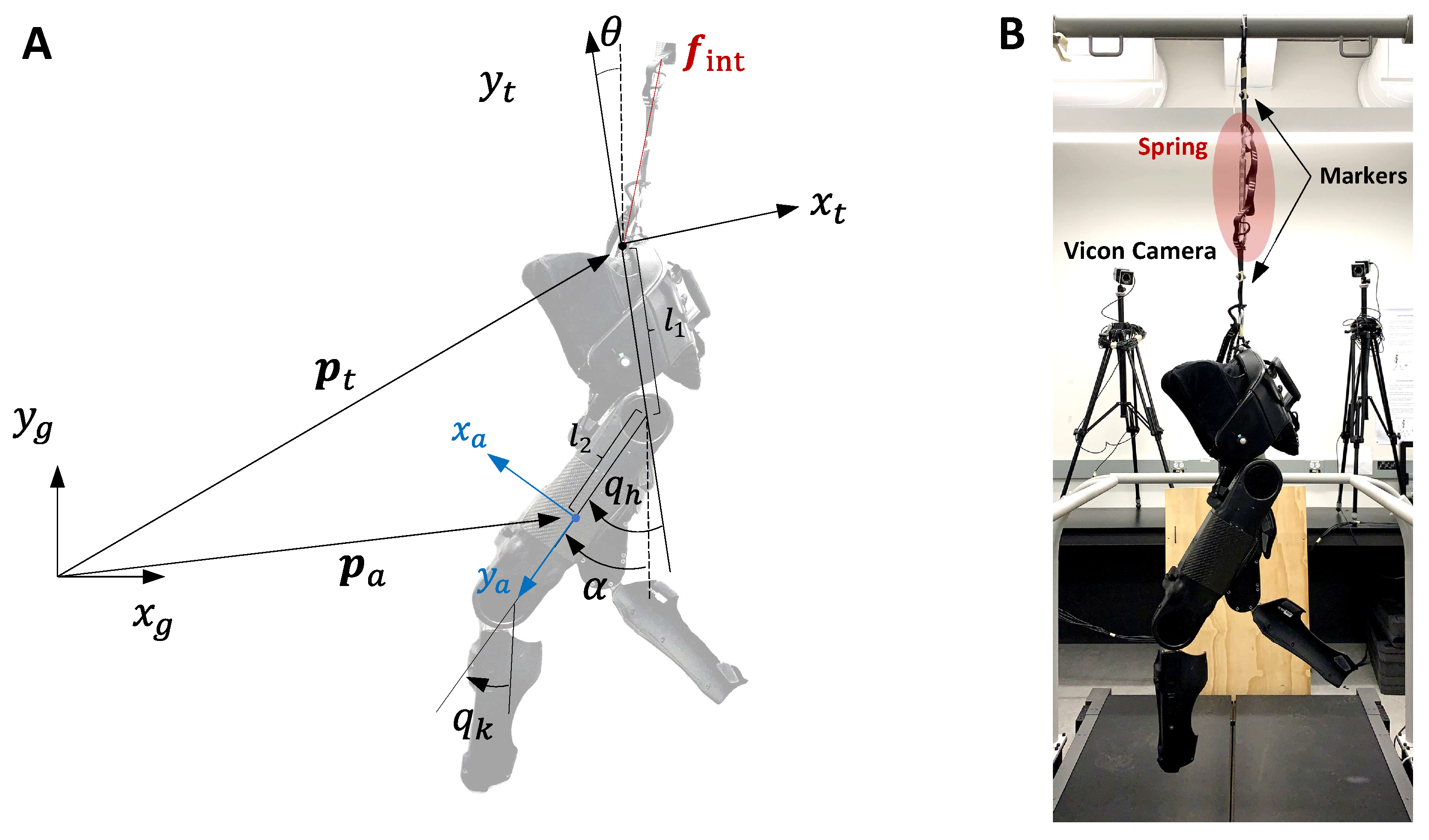
2.1. Interaction Torque Modeling

Figure 1A illustrates the Indego exoskeleton and its coordination systems in the sagittal plane. This lower limb exoskeleton has seven DOFs including one rotational and two translational DOFs of the trunk (three DOFs in total) with respect to the global frame and only four active DOFs of the exoskeleton knee and hip joints of the right and left legs. The exoskeleton also has two carbon–fiber ankle foot orthoses, which were removed from the exoskeleton due to their negligible mass. Given that the Indego exoskeleton does not have joints with off–sagittal–plane degrees of freedom (such as hip abduction and adduction DOFs) the off-sagittal dynamics of the exoskeleton during straight walking were negligible compared to its dynamics in the sagittal plane. The Indego lower–limb exoskeleton’s dynamics, with actuated hips and knees, in the presence of interaction forces and torques in the sagittal plane were considered as

$$\Gamma (\theta ,\dot{\theta },\ddot{\theta },\ddot{{\mathit{p}}_{\mathbf{1}}},\mathit{q},\dot{\mathit{q}},\ddot{\mathit{q}})={\mathit{u}}_{\mathrm{act}}+{\mathit{u}}_{\mathrm{int}}$$

(1)

where ${\mathit{p}}_{\mathbf{1}}=(p_{1,x};p_{1,y})\in {\mathbb{R}}^2$ and $\theta \in \mathbb{R}$ are the exoskeleton’s trunk segment position and orientation, respectively, described in the fixed global frame in the sagittal plane and ($\mathit{q}=[q_{h,r};q_{k,r};q_{h,l};q_{h,l}]\in {\mathbb{R}}^4$) consists of the exoskeleton right hip and knee joint angles followed by the left hip and knee joint angles. ${\mathit{u}}_{\mathrm{act}}=[{\mathbf{0}}_{3\times 1};{\mathit{\tau }}_{\mathrm{act}}]$ is the applied motor torques at the hip and knee joints of both legs (${\mathit{\tau }}_{\mathrm{act}}\in {\mathbb{R}}^4$). ${\mathit{u}}_{\mathrm{int}}=[{\mathit{f}}_{\mathrm{int}};m_{\mathrm{int}};{\mathit{\tau }}_{\mathrm{int}}]$ includes the interaction force (${\mathit{f}}_{\mathrm{int}}\in {\mathbb{R}}^2$) and moment ($m_{\mathrm{int}}\in \mathbb{R}$) applied to the exoskeleton trunk as well as the interaction torques applied to the exoskeleton joints (${\mathit{\tau }}_{\mathrm{int}}\in {\mathbb{R}}^4$). Finally, $\Gamma (.)$ represents the exoskeleton passive dynamics containing the inertial forces, centrifugal and Coriolis forces, and the forces due to gravity [24]. We note that ${\mathit{p}}_1$ and ${\dot{\mathit{p}}}_{\mathbf{1}}$ do not appear in $\Gamma$ as there are no forces being applied to the trunk due to the trunk linear position (${\mathit{p}}_{\mathbf{1}}$) and velocity($\dot{{\mathit{p}}_{\mathbf{1}}}$). Figure 1A provides a visual representation of the Indego lower-limb exoskeleton.

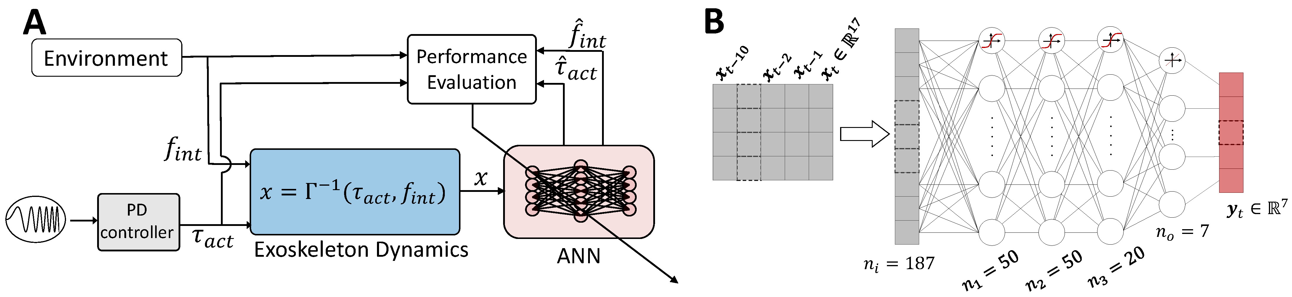
2.2. System Identification

To estimate the interaction forces and torques (${\mathit{u}}_{\mathrm{int}}$), we first identified the exoskeleton passive dynamics ($\Gamma$) without imposing any constraints on the system dynamics such as fixing the trunk segment. This was accomplished by hanging the exoskeleton from the ceiling by a spring with K = 1926.4 N/m, with reflective markers attached to both ends (Figure 1B). This way, we could measure the spring deflection and consequently compute the applied interaction force (${\mathit{f}}_{\mathrm{int}}$) accurately using Hooke’s law and a motion capture system consisting of eight Vero Cameras (Vicon, UK). Note that the absence of a human participant wearing the exoskeleton during the experiment did not hinder the identification of the exoskeleton passive dynamics as the measurements of the spring force and exoskeleton joint torques were sufficient for this purpose, without imposing any constraints on the system states. The identified exoskeleton passive dynamics could then be used to estimate the human–exoskeleton interaction.

The exoskeleton joints were excited in three different scenarios each for 500 s by applying chirp command trajectories controlled by joint–level PD controllers with $k_p$ = 1.5 N.m/deg and $k_d$ = 0.1 N.m.s/deg for the hip and $k_p$ = 0.2 N.m/deg and $k_d$ = 0.03 N.m.s/deg for the knee joint. Controller gains were obtained by trial and error to achieve a maximum tracking error of less than 10 degrees for the hip and 5 degrees for the knee joint during the experiment. The chirp commands had unique initial and final frequencies to prevent phase lock between joints (see Figure 2). The chirp signals were designed to cover at least 80% of each joint range of motion with frequencies between 0.2 to 0.9 Hz covering the speed ranges below 1.4 m/s for healthy individuals [25]. The spring force measurement, as well as the exoskeleton data consisted of its joint angles ($\mathit{q}$), angular velocity ($\dot{\mathit{q}}$), the angle of each thigh with respect to the gravity vector ($\gamma \in \mathbb{R}$), the linear acceleration of each thigh ($\mathit{a}=[a_x;a_y]\in {\mathbb{R}}^2$), and the applied joint torques (${\mathit{\tau }}_{\mathrm{act}}$) were acquired at 200 Hz. By choosing different upchirp and downchirp rates for the command trajectories to each joint, we applied three different patterns for the interaction forces to the exoskeleton trunk. During the first scenario (training dataset), the right hip and left knee frequencies upchirped from 0.2 Hz to 0.9 Hz, while the left hip and right knee frequencies downchirped from 0.9 Hz to 0.2 Hz. All joints in the second scenario (validation) upchirped from 0.2 Hz to 0.9 Hz. Finally, in the last scenario (test), the joints on the right leg upchirped from 0.2 to 0.9 Hz while those on the left leg downchirped from 0.9 to 0.2 Hz. In all these cases, the frequency sweep rate for the upchirping or downchirping joints were selected slightly different to prevent phase locking between joints (Figure 2).

According to Equation (1), we then computed the trunk orientation ($\theta$) and its derivative in addition to its linear acceleration (${\ddot{\mathit{p}}}_1$) to train a data–driven model for the estimation of exoskeleton passive dynamics ($\Gamma$). Even though this information was not directly included in the exoskeleton measurements, they were obtained using either of the thigh’s linear accelerometer measurements ($\mathit{a}$) or through obtaining its angle ($\gamma$) with respect to the gravity vector ($\mathit{g}$). The trunk orientation was then computed using the angle ($\gamma$) and the corresponding hip joint angle (the angle between the thigh and the upper segment) measured using the motor encoders. Therefore, we drop the leg index hereafter. According to Figure 1A, we could simply obtain the trunk orientation as

$$\theta =q_h-\gamma .$$

(2)

To obtain ${\ddot{\mathit{p}}}_1$, we first mapped the thigh acceleration ($\mathit{a}$) from the thigh coordinate to the global coordinate frame. As the thigh coordinate frame (($x_2,y_2$)) rotated clockwise by $\pi -\gamma$ rad compared to the global frame ($(x_0,y_0)$), the linear acceleration measured in the thigh frame ($\mathit{a}$) could be mapped to the global frame as

$${\ddot{\mathit{p}}}_2=R_2^0\left(\gamma \right)\mathit{a}=\left[\begin{array}{cc}cos\left(\pi -\gamma \right)& -sin\left(\pi -\gamma \right)\\ sin\left(\pi -\gamma \right)& cos\left(\pi -\gamma \right)\end{array}\right]\mathit{a}=\left[\begin{array}{cc}-cos\left(\gamma \right)& -sin\left(\gamma \right)\\ sin\left(\gamma \right)& -cos\left(\gamma \right)\end{array}\right]\mathit{a}.$$

(3)

Moreover, the following equation holds between the origin of the trunk frame and the accelerometer position with respect to the global frame (${\mathit{p}}_2=(P_{2,x};p_{2,y})$)

$${\mathit{p}}_1=\left(\begin{array}{c}{p}_{2,x}+l_{2}sin\left(\gamma \right)-l_{1}sin\left(\theta \right)\\ p_{2,y}+l_{2}cos\left(\gamma \right)+l_{1}cos\left(\theta \right)\end{array}\right).$$

(4)

Taking the second derivative from the above equation and substituting Equation (3), we obtain

$${\ddot{\mathit{p}}}_1=\left(\begin{array}{c}{l}_2{s}_{\gamma }{\dot{\gamma }}^2+l_1{s}_{\theta }{\dot{\theta }}^2-c_{\gamma }{a}_x-s_{\gamma }{a}_y+\ddot{\gamma }{c}_{\gamma }{l}_2-c_{\theta }{l}_1\ddot{\theta }\\ -c_{\gamma }{l}_2{\dot{\gamma }}^2-c_{\theta }{l}_1{\dot{\theta }}^2-c_{\gamma }{a}_x-s_{\gamma }{a}_y-\ddot{\gamma }{l}_2{s}_{\gamma }-l_1{s}_{\theta }\ddot{\theta }\end{array}\right),$$

(5)

where $c_x$ and $s_x$ are shorthanded versions of $sin\left(x\right)$ and $cos\left(x\right)$, respectively. According to Equations (2) and (5), both $\theta$ and its derivatives, as well as ${\ddot{\mathit{p}}}_1$, could be obtained as a function of the exoskeleton joint angles ($\mathit{q}$), thigh accelerations ($\mathit{a}$), thigh orientation with respect to gravity ($\gamma$), and their derivatives. In other words, we have

$$[\theta ;\dot{\theta };\ddot{\theta };{\ddot{\mathit{p}}}_{\mathbf{1}}]=h(\gamma ,\dot{\gamma },\ddot{\gamma },\mathit{q},\dot{\mathit{q}},\ddot{\mathit{q}},\mathit{a}).$$

(6)

Henceforth, without loss of generality, we can consider $\Gamma$ as only a function of the exoskeleton measurements and rewrite Equation (1) as

$$\Gamma (\gamma ,\dot{\gamma },\ddot{\gamma },\mathit{q},\dot{\mathit{q}},\ddot{\mathit{q}},\mathit{a})={\mathit{u}}_{\mathrm{act}}+{\mathit{u}}_{\mathrm{int}}.$$

(7)

Therefore, we can use the thigh angle with respect to the gravity vector and its linear acceleration instead of the position and orientation of trunk segment to identify Equation (1). Moreover, we defined the origin of the exoskeleton’s trunk frame exactly at the point where the spring force was applied (Figure 1). This allowed us to consider $m_{\mathrm{int}}=0$. Equation (1) can thus be further simplified as

$$\Gamma \left(\mathit{x}\right)=\mathit{y},$$

(8)

where $\mathit{x}=[\gamma ;\dot{\gamma };\ddot{\gamma };\mathit{q};\dot{\mathit{q}};\ddot{\mathit{q}};\mathit{a}]\in {\mathbb{R}}^{17}$ and $\mathit{y}=[{\mathit{f}}_{\mathrm{int}};0;{\mathit{\tau }}_{\mathrm{act}}]\in {\mathbb{R}}^7$.

Various time–delay ANNs [26] with a tanh activation function (Figure 3B) were trained on the training dataset to learn the exoskeleton’s passive dynamics ($\widehat{\Gamma }\left(\mathit{x}\right)=\widehat{\mathit{y}}$) by minimizing the root mean squared error (RMSE) between the Z–score normalized measured ($\mathit{y}$) and estimated ($\widehat{\mathit{y}}$) forces and torques (Figure 3A) using the scaled conjugate gradient backpropagation algorithm [27]. The training was stopped when 10 consecutive iterations did not improve the performance of the ANN on the validation dataset. Different combinations of network structure (ranging from a single hidden layer with 10 neurons to three hidden layers with 250 neurons in total), number of input delays (ranging from 0 to 50 samples), and $L^2$ weight regularization factors (ranging from 0 to 0.5) were evaluated according to (Figure 4A), by training each network five times and computing their mean performance on the validation dataset to compare networks and to obtain the best architecture.

2.3. Experimental Estimation of Human–Exoskeleton Interaction Torque

We estimated the human–exoskeleton interaction torques by conducting experiments on three able–bodied participants. Interaction torques were estimated in real time using the exoskeleton measurements fed to the N9 network implemented on a real–time kernel using MATLAB Simulink Desktop Real–time toolbox running at 200 Hz. The participants included two 22–year–old males with heights of 180 cm and 182 cm, and body masses of 82 kg and 90 kg, respectively, and a 24–year–old female with a height of 174 cm and body mass of 68 kg. They walked on a treadmill at slow (0.4 m/s), medium (0.6 m/s), and fast (0.8 m/s) speeds while wearing a passive exoskeleton. All participants had no known musculoskeletal impairments and provided informed consent prior to the experiment. The study protocol and procedures were approved by the University of Waterloo Clinical Research Ethics Committee (ORE#41794) and conformed to the Declaration of Helsinki.

Knowing the exoskeleton passive dynamics, we could estimate the human–exoskeleton interaction forces and torques using Equation (1) as

$${\mathit{u}}_{\mathrm{int}}=\widehat{\Gamma }\left(\mathit{x}\right)-{\mathit{u}}_{\mathrm{act}}=\widehat{\mathit{y}}-{\mathit{u}}_{\mathrm{act}}.$$

(9)

In this case, since the exoskeleton motors applied no torques (${\mathit{u}}_{act}=0$), the estimated interaction torques were obtained as ${\mathit{u}}_{int}=\widehat{\Gamma }$.

3. Results and Discussion

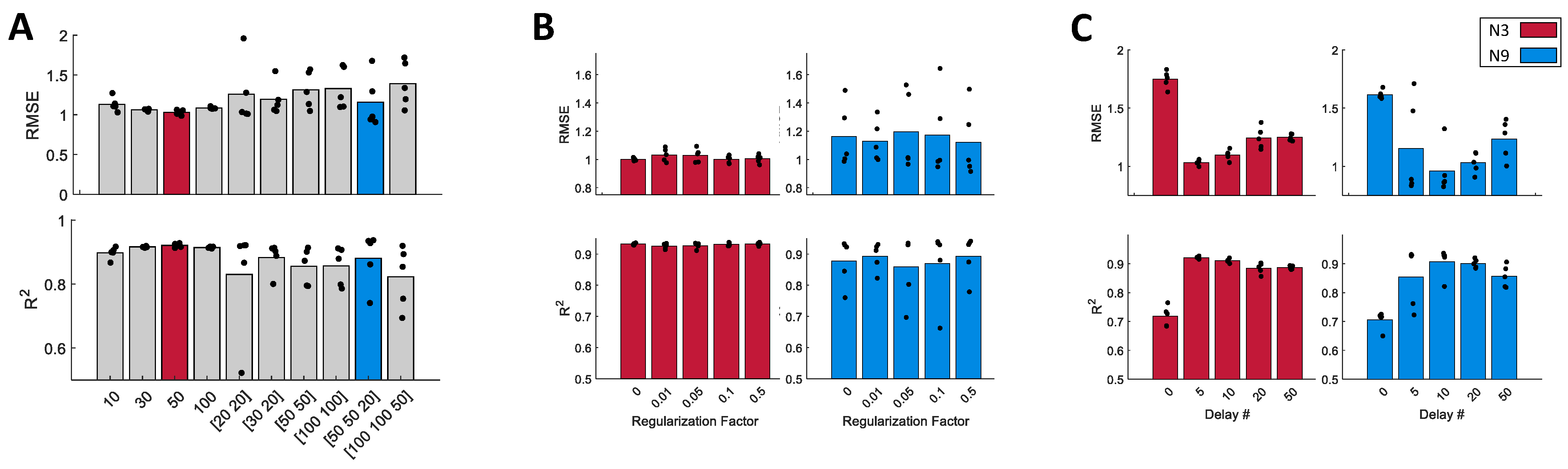
3.1. Tuning the Network Structure and Hyperparameters

To tune the network structure and complexity, we trained ten networks with complexities ranging from a single hidden layer with 10 neurons up to a network with three hidden layers with 250 neurons in total. Figure 4A shows the average RMSE and the coefficient of determination ($R^2$) computed using each of the trained networks on the validation datasets. The training procedure was repeated five times for each network to account for the randomness of the training process without a regularization coefficient and with input delays equal to five. Our results indicated that the average test performance dropped as the network complexity increased. This was indicated by the increase in the average RMSE and the decrease in the average adjusted $R^2$ after N3 (the third network denoted by red in Figure 4A), which resulted in one of the best performance results consistently in all five training trials (RMSE = 1.03 $R^2=0.92$). On the other hand, the RMSE and $R^2$ variations on the validation dataset also increased with the network complexity. This can be explained by the association between the networks’ expressiveness and overfitting. N9 (the ninth network denoted by blue in the same graph), for example, obtained one of the best validation performance results among all networks three out of five times. To further improve the results, the training procedure was repeated for N3 and N9 with regularization coefficients ranging from 0 to 0.5 and with different numbers of input delays ranging from 0 to 50 samples equal to 0–250 ms.

Figure 4B investigates the effect of the regularization coefficient on N3 and N9’s performance results, indicating that increasing the regularization coefficient improved neither the network performance in the case of N3 nor the consistency of the validation results in case of N9. The number of input delays, on the contrary, showed to be effective in enhancing both networks’ performance. According to Equation (8), providing ANNs with histories of $\mathit{x}$ would not be effective as $\Gamma$ is solely a function of $\mathit{x}$. However, the best performance for N3 was obtained with 5 input delays (RMSE = 0.99 and $R^2$ = 0.92), while N9’s best performance was obtained with 10 input delays (RMSE = 0.82 and $R^2=0.93$). The underlying reason was that by adding input delays, the ANNs could learn to smooth the input data and therefore become less sensitive to the input noise. The more flexible structure of N9 enabled it to benefit from the additional information embedded in the input history, while N3’s capacity became saturated with more than five input delays, and therefore, N9 was able to reach a less biased performance. Hence, we chose N9 consisting of three hidden layers each with 50, 50, and 20 neurons, respectively, with 10 input delays, for the estimation of the exoskeleton dynamics.

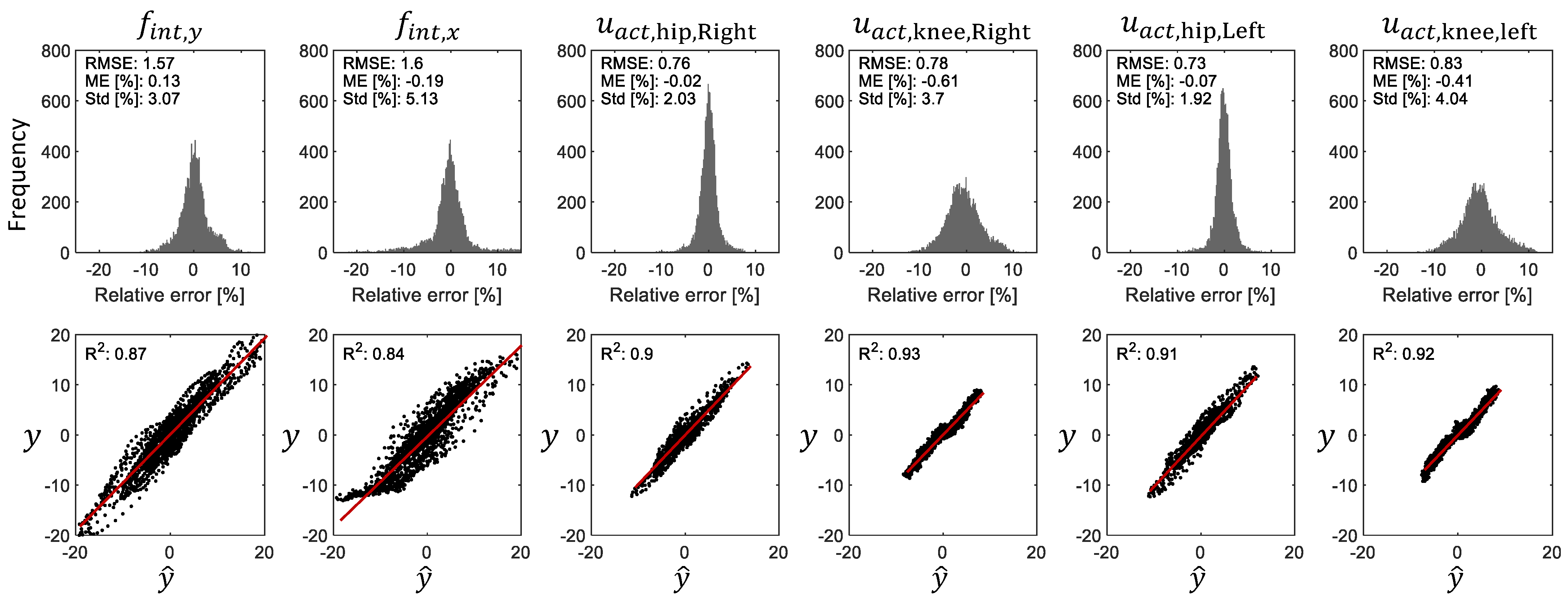
3.2. N9 Performance on Test Dataset

The overall RMSE of N9 on the test dataset was 1.23 and $R^2$ = 0.89. Figure 5 shows the test performance of N9 for each output channel. The relative error was computed by normalizing the estimation error over the maximum range of each output channel. For example, according to Figure 2, the range of $f_{int,y}$ was about 200 N. In that case, 1% of relative error means 2 N of force estimation error. The trained network exhibited an accurate estimation of the applied exoskeleton joint torques with a coefficient of determination greater than 0.9. The knee torque estimation was slightly more biased compared to the hip due to the more pronounced static friction at the knee. Particularly, at lower speeds, the larger mass (4.7 kg) of the thigh segment dominated the static friction of the motor gears at the hip joint, resulting in a more predictable dynamical behavior. The light weight of the shank segments, in contrast, was negligible (0.6 kg) compared to the static friction and motor backlash, causing a greater estimation bias at the knee. This was evident from the dead zone–like behavior emerging in the y–$\widehat{y}$ graphs for the knees. At the higher speeds when static friction was dominated by inertial and damping torques, the knee torque estimations were more accurate than the hip joint due to its smaller moment of inertia leading to a higher coefficient of determination at the knee joint. The RMSE value for the interaction forces was higher than the joint torques. Simplifying the exoskeleton dynamics into the sagittal plane was the main reason behind this, as our model could not represent the applied interaction force to the exoskeleton trunk in the z direction. The external forces were also estimated with an RMSE smaller than 1.6 with a negligible bias (ME < 0.2%).

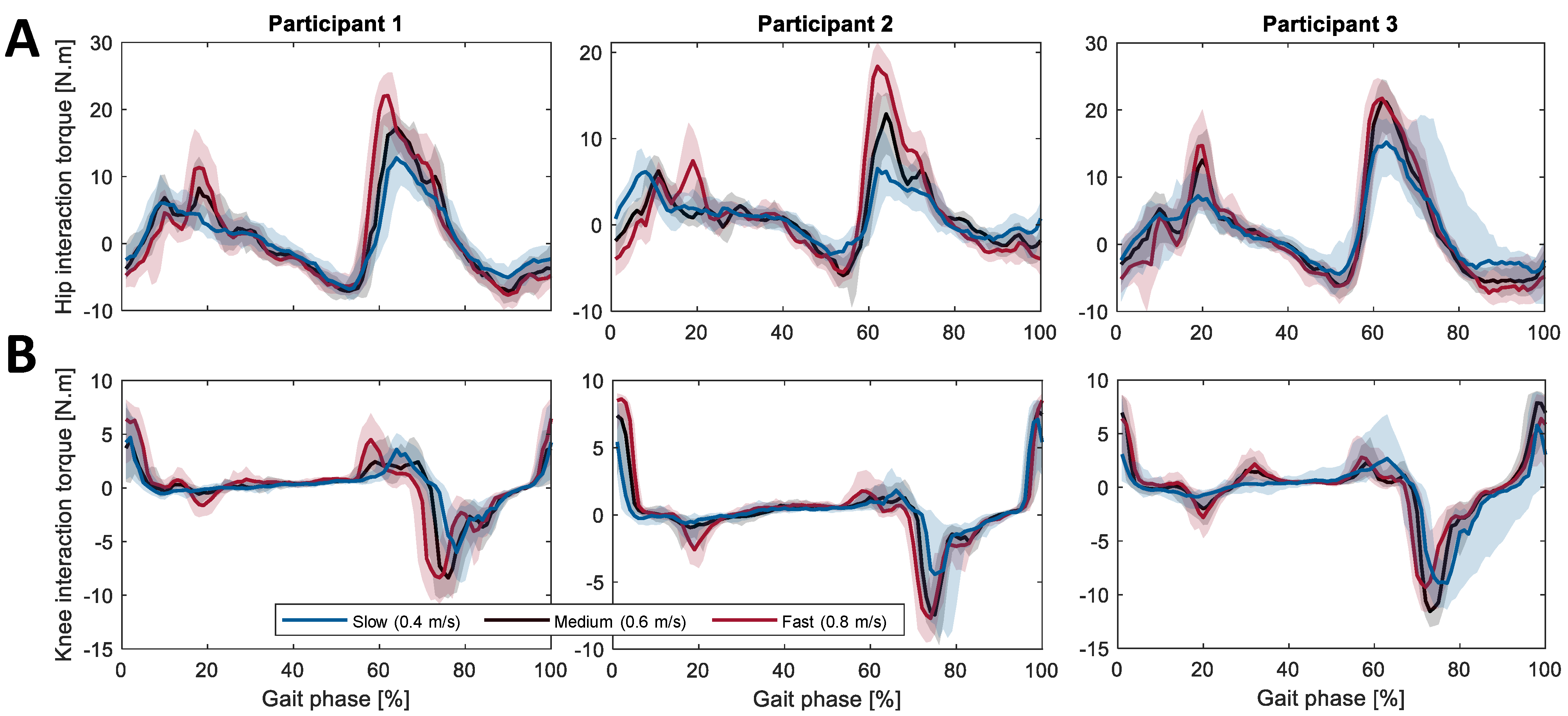
3.3. Human–Exoskeleton Interaction Torque Estimation

The estimated interaction torques at the hip and knee joints of the right leg are presented for three participants walking on a treadmill at slow, medium, and fast speeds in Figure 6. The estimated torques are plotted against the estimated gait phase [28], i.e., a gait–cycle–based monotonic measure often defined based on gait events such as heel strike and used to elucidate the evolution of the gait cycle [29]. The results showed a similar behavior in the estimated interaction torques at both joints regardless of the participant and walking speed. As expected, the magnitude of the interaction torques at both joints increased as the walking speed increased. At the knee joint (Figure 6B), a large peak during the late swing and early stance phase (about 10% of the gait cycle) indicated that the interaction torque was in favor of a knee flexion for damping the knee ballistic swing before the heel strike and stabilizing the knee after the heel strike. In the late stance and early swing phases (approximately 60% of the gait cycle), a negative interaction torque peak was in the direction of a knee extension, which was required to throw the exoskeleton shank segment forward during the swing phase.

At the hip joint (Figure 6A), a relatively large peak occurred during the late stance phase, indicating that the user torque tended to flex the exoskeleton hip joint. Similarly, a less pronounced and unexpected peak was also exhibited in the early stance phase. This was surprising since the hip joint typically extends during this phase, leading to an anticipated negative interaction torque. To better understand this observation, it was necessary to consider the left hip gait phase and its interaction torque. During the early stance phase of the right leg, the left leg was in its early swing phase, applying a large positive interaction torque to the left joints of the exoskeleton. Since the trunk segment of the exoskeleton was shared between the right and left thigh segments, the isolation of those two interaction torques was not fully possible, leading to a leakage of interaction torques between the left and right hip joints of the exoskeleton. Consequently, the large positive flexion torque of the left hip manifested itself in the estimated interaction torque at the right hip, and vice versa when the left leg was in the early stance phase.

4. Conclusions

The dynamics of a lower–body exoskeleton were identified and used for the estimation of the human–exoskeleton interaction torques. An exoskeleton was hung using a linear spring allowing us to measure the exoskeleton–environment interaction forces by motion capture. Meanwhile, exoskeleton joints were excited with different chirp commands designed to cover the range of motion of all joints in three scenarios, each used either for the training, validation, or test of data–driven models. Various time–delay ANNs were trained and validated on the collected datasets and the network structure, the number of input delays, and regularization factors were tuned according to their validation performance. Testing results indicated an accurate performance of the exoskeleton joint torque estimation (RMSE < 0.85, ME < 0.6%, and $R^2$ > 0.9) as well as an acceptable performance of the interaction force estimation (RMSE < 1.6, $R^2$ > 0.84). One of the challenges of the presented method was the redundancy between the estimated interaction torques at the left and right hips due to sharing the trunk segment. Modeling the exoskeleton motion in the sagittal plane is another limitation of this work. Even though a high accuracy in the joint torque estimation was obtained, with more accurate modeling of the exoskeleton in 3D space, we could model the interaction forces applied to the exoskeleton better. Developing a driftless trunk orientation estimation method is another challenge in this regard, which is required for monitoring the orientation of the exoskeleton trunk in 3D space continuously. Despite these challenges, this direction will have implications for building a data–driven ground reaction force estimator in our future work or using force–plate–free predictions of joint net torques [30]. Our next step, however, is to integrate the identified exoskeleton dynamics in our adaptive trajectory and feed–forward controllers [31,32], which were only tested in simulation due to the lack of ability to estimate the human–exoskeleton interaction torques.

References

1. Duschau-Wicke, A.; Von Zitzewitz, J.; Caprez, A.; Lunenburger, L.; Riener, R. Path control: A method for patient-cooperative robot-aided gait rehabilitation. IEEE Trans. Neural Syst. Rehabil. Eng. 2009, 18, 38–48. [Google Scholar] [CrossRef] [PubMed] [Green Version]
2. Huang, V.S.; Krakauer, J.W. Robotic neurorehabilitation: A computational motor learning perspective. J. Neuroeng. Rehabil. 2009, 6, 5. [Google Scholar] [CrossRef] [Green Version]
3. Moreno, J.C.; Asin, G.; Pons, J.L.; Cuypers, H.; Vanderborght, B.; Lefeber, D.; Ceseracciu, E.; Reggiani, M.; Thorsteinsson, F.; Del-Ama, A.; et al. Symbiotic wearable robotic exoskeletons: The concept of the biomot project. In Proceedings of the International Workshop on Symbiotic Interaction, Helsinki, Finland, 30–31 October 2014; Springer: Berlin/Heidelberg, Germany, 2015; pp. 72–83. [Google Scholar]
4. Murray, S.A.; Ha, K.H.; Hartigan, C.; Goldfarb, M. An assistive control approach for a lower-limb exoskeleton to facilitate recovery of walking following stroke. IEEE Trans. Neural Syst. Rehabil. Eng. 2014, 23, 441–449. [Google Scholar] [CrossRef] [PubMed]
5. Riener, R.; Lunenburger, L.; Jezernik, S.; Anderschitz, M.; Colombo, G.; Dietz, V. Patient-cooperative strategies for robot-aided treadmill training: First experimental results. IEEE Trans. Neural Syst. Rehabil. Eng. 2005, 13, 380–394. [Google Scholar] [CrossRef]
6. Banala, S.K.; Agrawal, S.K.; Scholz, J.P. Active Leg Exoskeleton (ALEX) for gait rehabilitation of motor-impaired patients. In Proceedings of the 2007 IEEE 10th International Conference on Rehabilitation Robotics, Noordwijk, The Netherlands, 13–15 June 2007; IEEE: Piscataway, NJ, USA, 2007; pp. 401–407. [Google Scholar]
7. Zhang, J.f.; Dong, Y.m.; Yang, C.j.; Geng, Y.; Chen, Y.; Yang, Y. 5-Link model based gait trajectory adaption control strategies of the gait rehabilitation exoskeleton for post-stroke patients. Mechatronics 2010, 20, 368–376. [Google Scholar] [CrossRef]
8. Li, Y.; Sena, A.; Wang, Z.; Xing, X.; Babic, J.; van Asseldonk, E.H.; Burdet, E. A review on interaction control for contact robots through intent detection. Prog. Biomed. Eng. 2022, 4, 032004. [Google Scholar] [CrossRef]
9. Li, Y.; Ganesh, G.; Jarrassé, N.; Haddadin, S.; Albu-Schaeffer, A.; Burdet, E. Force, impedance, and trajectory learning for contact tooling and haptic identification. IEEE Trans. Robot. 2018, 34, 1170–1182. [Google Scholar] [CrossRef] [Green Version]
10. Losey, D.P.; McDonald, C.G.; Battaglia, E.; O’Malley, M.K. A review of intent detection, arbitration, and communication aspects of shared control for physical human–robot interaction. Appl. Mech. Rev. 2018, 70, 010804. [Google Scholar] [CrossRef] [Green Version]
11. De Rossi, S.M.M.; Vitiello, N.; Lenzi, T.; Ronsse, R.; Koopman, B.; Persichetti, A.; Vecchi, F.; Ijspeert, A.J.; Van der Kooij, H.; Carrozza, M.C. Sensing pressure distribution on a lower-limb exoskeleton physical human-machine interface. Sensors 2010, 11, 207–227. [Google Scholar] [CrossRef]
12. Shojaei Barjuei, E.; Caldwell, D.G.; Ortiz, J. Bond graph modeling and kalman filter observer design for an industrial back-support exoskeleton. Designs 2020, 4, 53. [Google Scholar] [CrossRef]
13. Jezernik, S.; Colombo, G.; Morari, M. Automatic gait-pattern adaptation algorithms for rehabilitation with a 4-DOF robotic orthosis. IEEE Trans. Robot. Autom. 2004, 20, 574–582. [Google Scholar] [CrossRef]
14. Katsura, S.; Matsumoto, Y.; Ohnishi, K. Modeling of force sensing and validation of disturbance observer for force control. IEEE Trans. Ind. Electron. 2007, 54, 530–538. [Google Scholar] [CrossRef]
15. Liang, C.; Hsiao, T. Admittance control of powered exoskeletons based on joint torque estimation. IEEE Access 2020, 8, 94404–94414. [Google Scholar] [CrossRef]
16. Sharifi, M.; Mehr, J.K.; Mushahwar, V.K.; Tavakoli, M. Autonomous Locomotion Trajectory Shaping and Nonlinear Control for Lower Limb Exoskeletons. IEEE/ASME Trans. Mechatron. 2022, 27, 645–655. [Google Scholar] [CrossRef]
17. Ghan, J.; Kazerooni, H. System identification for the Berkeley lower extremity exoskeleton (BLEEX). In Proceedings of the 2006 IEEE International Conference on Robotics and Automation, ICRA 2006, Orlando, FL, USA, 15–19 May 2006; IEEE: Piscataway, NJ, USA, 2006; pp. 3477–3484. [Google Scholar]
18. Chen, L.; Wang, C.; Song, X.; Wang, J.; Zhang, T.; Li, X. Dynamic trajectory adjustment of lower limb exoskeleton in swing phase based on impedance control strategy. Proc. Inst. Mech. Eng. Part I J. Syst. Control Eng. 2020, 234, 1120–1132. [Google Scholar] [CrossRef]
19. Yan, Y.; Chen, Z.; Huang, C.; Chen, L.; Guo, Q. Human-exoskeleton coupling dynamics in the swing of lower limb. Appl. Math. Model. 2022, 104, 439–454. [Google Scholar] [CrossRef]
20. Zha, F.; Sheng, W.; Guo, W.; Qiu, S.; Deng, J.; Wang, X. Dynamic parameter identification of a lower extremity exoskeleton using RLS-PSO. Appl. Sci. 2019, 9, 324. [Google Scholar] [CrossRef] [Green Version]
21. Vaney, C.; Gattlen, B.; Lugon-Moulin, V.; Meichtry, A.; Hausammann, R.; Foinant, D.; Anchisi-Bellwald, A.M.; Palaci, C.; Hilfiker, R. Robotic-assisted step training (lokomat) not superior to equal intensity of over-ground rehabilitation in patients with multiple sclerosis. Neurorehabilit. Neural Repair 2012, 26, 212–221. [Google Scholar] [CrossRef] [PubMed]
22. Farris, R.J.; Quintero, H.A.; Murray, S.A.; Ha, K.H.; Hartigan, C.; Goldfarb, M. A preliminary assessment of legged mobility provided by a lower limb exoskeleton for persons with paraplegia. IEEE Trans. Neural Syst. Rehabil. Eng. 2013, 22, 482–490. [Google Scholar] [CrossRef] [PubMed] [Green Version]
23. Sharifi, M.; Mehr, J.K.; Mushahwar, V.K.; Tavakoli, M. Adaptive cpg-based gait planning with learning-based torque estimation and control for exoskeletons. IEEE Robot. Autom. Lett. 2021, 6, 8261–8268. [Google Scholar] [CrossRef]
24. Spong, M.W. Modeling and control of elastic joint robots. J. Dyn. Sys. Meas. Control 1987, 109, 310–318. [Google Scholar] [CrossRef]
25. McCrum, C.; Lucieer, F.; van de Berg, R.; Willems, P.; Pérez Fornos, A.; Guinand, N.; Karamanidis, K.; Kingma, H.; Meijer, K. The walking speed-dependency of gait variability in bilateral vestibulopathy and its association with clinical tests of vestibular function. Sci. Rep. 2019, 9, 18392. [Google Scholar] [CrossRef] [PubMed] [Green Version]
26. Waibel, A.; Hanazawa, T.; Hinton, G.; Shikano, K.; Lang, K.J. Phoneme recognition using time-delay neural networks. IEEE Trans. Acoust. Speech Signal Process. 1989, 37, 328–339. [Google Scholar] [CrossRef]
27. Møller, M.F. A scaled conjugate gradient algorithm for fast supervised learning. Neural Netw. 1993, 6, 525–533. [Google Scholar] [CrossRef]
28. Shushtari, M.; Dinovitzer, H.; Weng, J.; Arami, A. Ultra-Robust Real-Time Estimation of Gait Phase. IEEE Trans. Neural Syst. Rehabil. Eng. 2022, 30, 2793–2801. [Google Scholar] [CrossRef]
29. Winter, D.A. Human balance and posture control during standing and walking. Gait Posture 1995, 3, 193–214. [Google Scholar] [CrossRef]
30. Dinovitzer, H.; Shushtari, M.; Arami, A. Accurate Real-Time Joint Torque Estimation for Dynamic Prediction of Human Locomotion. IEEE Trans. Biomed. Eng. 2023. [Google Scholar] [CrossRef]
31. Shushtari, M.; Nasiri, R.; Arami, A. Online reference trajectory adaptation: A personalized control strategy for lower limb exoskeletons. IEEE Robot. Autom. Lett. 2021, 7, 128–134. [Google Scholar] [CrossRef]
32. Nasiri, R.; Shushtari, M.; Arami, A. An adaptive assistance controller to optimize the exoskeleton contribution in rehabilitation. Robotics 2021, 10, 95. [Google Scholar] [CrossRef]
Figure 1. (A) The exoskeleton coordinates and joint angles. The global, trunk, and thigh frames are denoted by 0, 1, and 2 indices, respectively. The trunk and thigh angles with respect to the gravity vector are denoted by θ and γ , respectively. q h and q k represent the hip and knee joint angles, respectively. p 1 and p 2 show the position of the trunk and thigh coordinated in the global frame (( x 0 , y 0 )). In blue, the acceleration vector ( a ) measured by the accelerometer embedded in the exoskeleton’s thigh is plotted against the thigh frame. In red, we plotted the interaction force vector ( f int ) calculated from the linear spring’s deflection measured by motion capture. The distance from the trunk frame origin to the hip joint rotation axis and from there to the accelerometer location on the exoskeleton’s thigh is indicated by l 1 and l 2 , and the gravity axis is illustrated by dashed lines. (B) The exoskeleton in hung position during data collection for dynamics identification. Joints are excited during the experiment while the exoskeleton interaction with the environment is limited to the force applied through a linear spring with reflective markers on both ends enabling us to measure the spring deflection using a motion capture system and, consequently, the applied force.
Robotics 12 00066 g001
Figure 2. The hip and knee excitation torques applied to the left and right exoskeleton legs, as well as the interaction force on the y axis. During the generation of each of the training, validation, and test datasets, exoskeleton joints were activated with unique and different chirp commands resulting in different exoskeleton–environment interaction profiles.
Robotics 12 00066 g002
Figure 3. (A) Block diagram of the exoskeleton dynamic identification experiment. The interaction force ( f int ) is applied to the exoskeleton through a linear spring through which the exoskeleton is hung. Exoskeleton joints are controlled by chirp position commands using PD controllers applying the excitation torques ( τ act ) to the exoskeleton. Measurements of the exoskeleton (x), containing joint angles and their derivatives as well as the thigh angle with respect to the gravity vector and its linear acceleration, are fed to a neural network for the estimation of the interaction force ( f ^ int ) and motor torques ( τ ^ act ), which are then compared to their actual values. The estimation error is then used to update the neural network weights to improve its estimation accuracy. (B) Structure of a time–delay neural network with 10 input delays and 3 hidden layers with 50, 50, and 20 neurons, respectively, with a t a n h activation function.
Robotics 12 00066 g003
Figure 4. (A) Validation performance of ANNs with 10 different structures in terms of RMSE and adjusted R 2 computed on the Z–normalized data. The training procedure was repeated 5 times for each structure to study the sensitivity of the training procedure to the network’s initial weight for each structure. Each validation performance is denoted by a black dot while the average performance is denoted by bars. The training was conducted with 5 input delays and no regularization. N3 (denoted by red) and N9 (denoted by blue) demonstrated a better performance compared to the other networks. N9, however, exhibited more variability across training repetitions. Those networks were selected for further analysis to investigate the effect of regularization factor and the number of input delays. (B) Comparison of N3 and N9 performance across different selections of regularization factors. The variation of the N9 performance across training repetitions is unaffected by regularization. (C) Effect of the number of input delays on the N3 and N9 networks’ performance. N3 has the best performance with 5 input delays while N9 reaches the best performance at 10 input delays.
Robotics 12 00066 g004
Figure 5. The Test performance of N9 for each output channel. In the top row, the distribution of the estimation error of external force or joint applied torques relative to their peak–to–peak range is depicted. Interaction forces in the y and x direction exhibit a higher estimation error compared to those of the exoskeleton active joints. Applied torques to the hip joints, in particular, are estimated with a higher accuracy and smaller standard deviation. Even though knee joint applied torques are estimated with similarly small errors (small bias), they show a higher standard deviation associated to the more prominent role of static friction. The bottom row shows the correlation between the measured data and the N9 estimation for each output channel. The estimated outputs have a relatively lower coefficient of determination in case of interaction forces, while they show R 2 > 0.9 for the active joints of the exoskeleton.
Robotics 12 00066 g005
Figure 6. The estimated interaction torques at (A) the hip and (B) the knee joints of the right leg for three participants walking at different speeds (ranging from 0.4 m/s to 0.8 m/s) are shown. The values represent the average across different steps. The solid lines represent the median of the estimated interaction torque, while the shaded area represents the torques that fall within the 5th to 95th percentile. Positive torque values are in favor of joint flexion while negative values are in favor of joint extension.
Robotics 12 00066 g006
Disclaimer/Publisher’s Note: The statements, opinions and data contained in all publications are solely those of the individual author(s) and contributor(s) and not of MDPI and/or the editor(s). MDPI and/or the editor(s) disclaim responsibility for any injury to people or property resulting from any ideas, methods, instructions or products referred to in the content.