Article

An Optimal Control Approach to the Minimum-Time Trajectory Planning of Robotic Manipulators

Department of Industrial Engineering, University of Padova, Via Venezia, 1, 35131 Padua, Italy
*
Author to whom correspondence should be addressed.
Robotics 2023, 12(3), 64; https://doi.org/10.3390/robotics12030064
Submission received: 30 March 2023 / Revised: 21 April 2023 / Accepted: 26 April 2023 / Published: 28 April 2023
(This article belongs to the Topic Industrial Robotics: 2nd Volume)

Abstract

:
Trajectory planning is a classic problem in robotics, with different approaches and optimisation objectives documented in the literature. Most of the time, the path is assumed, i.e., pre-defined, and optimisation consists of finding the timing of motion under a number of constraints. The focus of this work is on the minimum-time manoeuvring of robotic manipulators. A nonlinear optimal control approach is proposed that does not require the provision of either a pre-defined path or a pre-defined control structure and allows the inclusion of dynamic constraints. The solution (path and timing of motion) is obtained by transforming the optimal control problem into a nonlinear programming problem. The proposed approach is applied to a two-link manipulator for illustration purposes. The optimisation is carried out both without and with obstacles. The minimum-distance and minimum-time solutions are compared, and some classic results are obtained, including the trapezoidal pattern of the joint velocity and the bang–bang structure of the control torques. The effects of limitations on the jerks of actuators and the rate of change in torque inputs are discussed. The application to a four-link manipulator is also included to show the ‘scalability’ of the approach, together with a comparison with a classic path-and-motion-planning method, to highlight the characteristics and performance of the proposed approach. Finally, the possibility of enforcing a number of via-points along the path is demonstrated. The proposed method allows the computation of the path and motion simultaneously with the computation time, which is 1–30 times the manoeuvre time, on a standard PC with the current implementation.

1. Introduction

Industry 4.0 is a term used to describe and encapsulate a set of technological changes in manufacturing that have been characterising and transforming the industry in the last several years [1,2,3]. Robotics and automation play a key role in this framework, with the motion optimisation and control of robotic manipulators under kinematic and dynamic constraints being one of the typical challenges.
Trajectory planning is a classic problem in robotics and is usually defined as finding the timing of the motion law along a given geometric path while satisfying certain requirements and minimising certain objectives. The typical objectives include execution time [4,5,6,7], vibrations [8,9] and energy consumption [10,11]. A general overview is given in [12]. All such approaches assume a pre-defined path, which is at least given in terms of so-called ‘via-points’, on top of which trajectory optimisation is performed.
The focus of this work is on the execution time of manipulators while accounting for both kinematic and dynamic constraints. An optimal control approach is employed while leaving the path among the optimisation variables. The optimisation problem is thus defined as finding the path, the timing of motion and related control inputs that are necessary to move the end-effector from the initial configuration to the final configuration in the minimum time while satisfying the kinematic and dynamic constraints.
Among the earliest attempts to solve the minimum-time problem for manipulators is [4]. After an unsuccessful attempt to tackle the problem directly with an optimal control approach, the solution was obtained by choosing the acceleration that made the velocity along the specified path as large as possible at every point without violating the constraints. A very similar approach was devised in [5]. In practice, the optimum is either the maximum acceleration or maximum deceleration, with the change between the two strategies taking place at switching points. One of the key issues is thus finding such points. In addition, for a given path, there is a maximum velocity curve (arising from the limited admissible torques), which complicates the problem. In [6], similar ideas are exploited, again based on the fact that, once the path is given, the problem becomes one-dimensional. In [7], a dynamics-based kinematic approach is proposed to compute the minimum-time trajectory. The method calculates the robot dynamics only at certain points, thus allowing online implementation, and was tested with 40 industrial manipulators. A mixed-integer optimal control problem was formulated in [13] to deal with multi-point manufacturing tasks, with a cubic polynomial between points. In such a scenario, it is necessary to plan the optimal strategy to traverse all the desired points in an orderly way while minimising the manoeuvre time.
It is interesting to note that the approach based on the switching points closely resembles the so-called ‘apex-finding’ method used to estimate the lap time of road vehicles [14,15] on a pre-defined path, where the switching points are named apex/critical points. The solution can also be obtained directly with an optimal control approach, which allows, among the other things, the control of abrupt changes at the switching points. However, a more general approach that does not require pre-defining the path, which thus becomes a result of optimisation, is also possible [15,16].
Similarly, in the robotic field, optimisation can also be carried out without pre-defining the path. An early example of such an application is discussed in [17], where the minimisation of the energy required to transfer the payload of a Cartesian manipulator while avoiding obstacles is considered. An optimal control approach was employed with barrier functions introduced into the cost function to prevent collisions. In [18], the minimum-time problem was solved by using an optimiser to vary the path, which was then used to feed the algorithm in [4], which computed the related execution time based on the maximum acceleration/maximum deceleration strategy. The computation of the optimal switching points was also the focus of [19], again under the assumption of a bang–bang control system, with application to a two-link manipulator with two control inputs. However, the optimal solution is not always purely bang–bang [20,21,22]. The rest-to-rest time-optimal manoeuvres of rigid two-link robotic manipulators was tackled in [23] using Pontryagin’s principle. The resulting two-point-boundary-value problem was solved using a combination of the forward–backward and shooting methods (i.e., indirect approach to the solution of the optimal control problem). In [24], the rest-to-rest time-optimal manoeuvre with no pre-defined trajectory and obstacle avoidance was considered. An optimal control problem was formulated and discretised on a fixed mesh to obtain a nonlinear programming problem (i.e., a direct approach was used). The method was applied to three-axis and six-axis manipulators.
Most of the minimum-time approaches proposed lead to discontinuous actuator torques. A limitation on the rate of change in torque was considered in [25], where the time-optimal point-to-point control of robot manipulators was solved as an optimal control problem. An indirect approach was employed. An iterative method for computing the optimal time based on decreasing the final time of the minimum-energy problem was proposed. An optimal control formulation, with the rate of change in motor torque as the input, was also employed in [26]. The related boundary value problem was discretised with equally spaced mesh points in the time domain. Penalty functions were employed to enforce constraints on the states and inputs. However, the cost function was not the time, but a convex combination of energy and power.
The perusal of the literature suggests that, in the most widespread approaches, path and motion planning are separate, with motion planning usually obtained with smooth functions, e.g., polynomial splines, through the via-points generated from the path planning. In this work, the problem of minimum-time trajectory planning without a pre-defined path is formulated as a nonlinear optimal control problem (OCP), where path and motion planning are solved simultaneously. In contrast to most of the approaches proposed in the literature, the optimal path is not given, since it is a result of optimisation. Therefore, via-points need not be defined. Additionally, the structure of the optimal control is not pre-defined, which is not the case for approaches that assume, e.g., maximum-acceleration/maximum-deceleration strategies. The effects of limitations on either the jerk of actuators or the rate of change in the control torque are also investigated in order to avoid the discontinuities (and related problems) that characterise many approaches. The dynamics of the system are included in the optimisation and affect the optimal path obtained. A direct solution approach is employed; i.e., the nonlinear OCP is transcribed to a nonlinear programming problem (NLP). A pseudo-spectral method is used: the discretisation is obtained with a collocation scheme, where the collocation points are the roots of Legendre polynomials and the solution is approximated with Lagrange polynomials. The approach has proven successful for solutions to large and nonlinear OCPs in the field of vehicle dynamics [15,27,28]. A mesh refinement scheme is employed, where both the mesh size and the order of the polynomial are varied during the iterations [29,30]. Automatic differentiation is used to compute the required derivatives [31].
This work is organised as follows. The OCP formulation is given in 
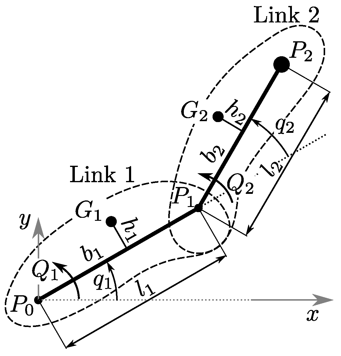
Section 2. The robotic manipulator model is illustrated in Section 3. The method is demonstrated in the case of kinematic constraints in Section 4, where minimum-time and minimum-path solutions, with and without obstacles, are discussed and compared.
The possibility of including a limitation on the joint jerk is shown in Section 4.3. The method proposed is also compared with the well-known Probabilistic Roadmap Method (PRM) [32,33] in Section 4.4. Dynamic constraints are introduced in Section 5, and trajectory planning is carried out again both with and without obstacles. In Section 5.3, the effect of limiting the rate of change in the joint torque to remove control discontinuities is addressed. The possibility of avoiding collisions with multiple obstacles is investigated in Section 5.4. In Section 5.5, optimisation is repeated while including a number of via-points: the path remains a result of optimisation (i.e., it is not pre-defined) but is enforced to satisfy the selected via-points. In Section 5.6, a redundant manipulator is considered in order to show the ‘scalability’ of the approach to more complex robots. Finally, in Section 6, some remarks on the numerics associated with the practical solutions of the optimisation problems discussed in the work are reported.

2. Optimal Control Problem Formulation

The dynamical system is described by a set of ordinary differential equations (ODEs):
x ̲ ˙ ( t ) = f ̲ ( x ̲ ( t ) , u ̲ ( t ) ) t i t t f ,
where x ̲ is the state, u ̲ is the input, t is the independent variable (for example, time), t i and t f are the related limits, and the dot denotes derivatives with respect to the independent variable. In the so-called Bolza form, the cost function, or performance index, is
J = M ( x ̲ ( t i ) , x ̲ ( t f ) ) + t i t f ( x ̲ ( t ) , u ̲ ( t ) ) d t .
where M and are the Mayer and Lagrange costs, respectively. The objective of the OCP is to minimise the cost function J while simultaneously satisfying the dynamic Equation (1) and the path constraints
c ̲ ( x ̲ ( t ) , u ̲ ( t ) ) 0 ̲ .
Finally, the boundary constraints are given by
b ̲ ( x ̲ ( t i ) , x ̲ ( t f ) ) = 0 ̲ ,
while the bounds on the controls are
| u ̲ ( t ) | u ̲ max
In the case of the robotic manipulator considered in this work, the cost function (2) consists of either the manoeuvre time or the travelled distance, while the path constraints (3) are both used to limit the maximum velocity, acceleration and torque of joints and to prevent collisions with obstacles. The solution of the problem consists of the path, the timing of motion and related control inputs.
The resulting continuous OCP is ‘transcribed’ to a nonlinear programming problem (NLP) through discretisation: a direct solution method is thus employed [15,28,34,35]. A collocation approach is used that produces an approximation of the solution in the form of polynomial functions. The problem equations are satisfied at collocation points. Among the different approaches available, in this work, the collocation points are obtained from the roots of Legendre polynomials, while Lagrange polynomials are used for approximations through collocation points. Hence, a Legendre–Gauss (LG) scheme is obtained. Among the different LG variants, the Legendre–Gauss–Radau (LGR) is used in this work. The solutions at all steps are obtained simultaneously by solving a set of algebraic equations. The transcription is carried out using GPOPS-II [36]. The resulting NLP is solved using the optimiser IPOPT [37].
A key aspect of efficiently generating accurate solutions to the OCP using collocation methods is the placement of both the mesh segment boundaries and the collocation points. In general, for each mesh interval of length h, there are p collocation points. Traditional fixed-order collocation methods determine the location of the mesh boundaries while keeping the degree p of the approximating polynomial fixed: these are called h-type methods. In contrast, p-type methods use a fixed mesh in combination with variable-order approximating polynomials. When both h and p are varied, the algorithm is of the h p type. As a general rule, if the error across a particular segment is large and uniformly distributed, the polynomial order should be increased. If a significant error occurs at an isolated point within a segment, the segment should be subdivided. In this work, the h p algorithm in [36] is used.
NLP solvers usually require derivatives of the cost function and constraints with respect to both the state and control variables. There are at least four possible approaches: computing derivatives analytically; computing derivatives numerically using finite-difference approaches; using complex-step differentiation [38,39,40]; and using algorithmic or automatic differentiation (AD). In order to compute function derivatives to machine precision without the need to derive them symbolically, the AD approach in [31] is used in this work.

3. Manipulator Model

The two-link planar manipulator shown in Figure 1 is considered in this work as an example of the application of the approach. The two degrees of freedom consist of the rotation q 1 of the first link with respect to the ground and the rotation q 2 of the second link with respect to the first link. The dataset employed is identical to that reported in [25] and is shown in Table 1.

3.1. Kinematic Model

The coordinates of a point P belonging to the second link are given by
x P ( q ̲ , ζ ) y P ( q ̲ , ζ ) = l 1 cos q 1 + ζ l 2 cos ( q 1 + q 2 ) l 1 sin q 1 + ζ l 2 sin ( q 1 + q 2 ) ,
where q ̲ = { q 1 , q 2 } T and ζ [ 0 , 1 ] . In particular, P 1 is obtained with ζ = 0 , and P 2 (end-effector) is obtained with ζ = 1 .

3.2. Dynamic Model

The equations of motion are obtained from the Lagrangian L = T V , where T and V are the kinetic and potential energies of the system. The kinetic energy is given by
T = 1 2 m 1 | v ̲ G 1 | 2 + 1 2 I 1 q ˙ 1 2 + 1 2 m 2 | v ̲ G 2 | 2 + 1 2 I 2 ( q ˙ 1 + q ˙ 2 ) 2 + 1 2 M | v ̲ P 2 | 2 ,
where m 1 and m 2 are the masses of the two links, I 1 and I 2 are the moments of inertia, M is the mass of the payload, v ̲ G 1 and v ̲ G 2 are the velocities of the centre of mass of the two links, and v ̲ P 2 is the velocity of the end-effector. The potential energy is V = 0 because the system is planar. The torques Q ̲ applied to the links are (see Figure 1)
Q ̲ = Q 1 , Q 2 T
Lagrange’s equations of motion are obtained from
d d t L q ˙ 1 L q 1 = Q 1 ,
d d t L q ˙ 2 L q 2 = Q 2 ,
which can be rewritten as
M ( q ̲ ) q ¨ ̲ + c ̲ ( q ̲ , q ˙ ̲ ) = Q ̲ ,
where M is a 2 × 2 matrix, while c ̲ is a 2 × 1 vector:
M ( q ̲ ) = m 11 m 12 m 12 m 22 ,
c ̲ ( q ̲ , q ˙ ̲ ) = l 1 q ˙ 2 ( 2 q ˙ 1 + q ˙ 2 ) ( m 2 h 2 cos q 2 + m 2 b 2 sin q 1 + M l 2 sin q 2 ) l 1 q ˙ 1 2 ( m 2 h 2 cos q 2 + m 2 b 2 sin q 1 + M l 2 sin q 2 ) ,
with
m 11 = I 1 + I 2 + m 1 ( b 1 2 + h 1 2 ) + m 2 ( l 1 2 + b 2 2 + h 2 2 + 2 l 1 b 2 cos q 2 2 l 1 h 2 sin q 2 ) +
M ( l 1 2 + l 2 2 + 2 l 1 l 2 cos q 2 ) ,
m 12 = I 2 + m 2 ( b 2 2 + h 2 2 + l 1 b 2 cos q 2 l 2 h 2 sin q 2 ) + M ( l 2 2 + l 1 l 2 cos q 2 )
m 22 = I 2 + m 2 ( b 2 2 + h 2 2 ) + M l 2 2 .

4. Planning with Kinematic Constraints

The planning problem needs to account for a number of constraints. Joint motors are typically limited in their maximum velocities. The associated constraints are given by
| q ˙ 1 | q ˙ 1 , max | q ˙ 2 | q ˙ 2 , max ,
where q ˙ 1 , max = 3 rad/s and q ˙ 2 , max = 8 rad/s are the values chosen in this work (estimated from [25]). Similarly, acceleration constraints can be included:
| q ¨ 1 | q ¨ 1 , max | q ¨ 2 | q ¨ 2 , max .
The initial and final positions of the joints provide the following boundary conditions:
q ̲ ( t i ) = { q 1 i , q 2 i } T q ̲ ( t f ) = { q 1 f , q 2 f } T .
The initial and final positions can alternatively be given in terms of Cartesian coordinates. However, the corresponding joint positions (19) can be readily obtained from Cartesian coordinates through inverse kinematics using (6). The advantage of defining the initial and final positions directly with (19) is also that the preferred manipulator configuration { q 1 , q 2 } T is selected among the multiple configurations that provide the same end-effector position { x P 2 , y P 2 } T . The initial and final velocities are zero ( q ˙ ̲ ( t i ) = q ˙ ̲ ( t f ) = 0 
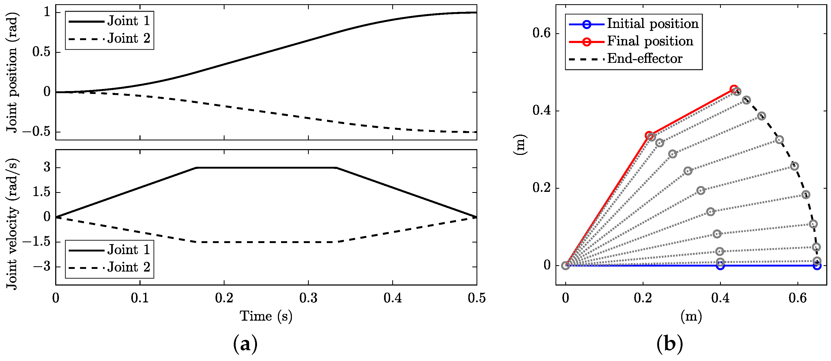
); i.e., rest-to-rest manoeuvres are considered. In the example of the application discussed in this work, the boundary conditions are q 1 i = q 2 i = 0 , q 1 f = 1 rad and q 2 f = −0.5 rad (see Figure 2b).
The speed coefficient c v is a typical index used to characterise the motion of joints:
c v = q ˙ max Δ q / T ,
where Δ q is the amplitude of motion, and T is the motion time. In several applications, a symmetric trapezoidal law is assumed for the velocities of joints, which also gives
c v = T T T a ,
where T a is the acceleration/deceleration time. The combination of (20) and (21) provides the expression of the maximum acceleration:
q ¨ max = q ˙ max 2 ( c v 1 ) Δ q .
A typical value for the speed coefficient is c v = 1.5 [41], which can be introduced in (22) to provide 18 and 128 rad/s 2 for the maximum accelerations of joint 1 and joint 2, respectively. The limit is assumed to be the minimum between the two, i.e., q ¨ 1 , max = q ¨ 2 , max = 18 rad/s 2 . It is worth stressing that the trapezoidal law is not enforced in the subsequent optimisation, although it is used to determine reasonable values for the maximum acceleration of joints allowed.

4.1. Minimum Time vs. Minimum Distance

The OCP is solved with M = 0 and = 1 in (2), with time t as the independent variable. Of course, one can equivalently use M = t f and = 0 . The controls are the accelerations u ̲ = { a q 1 , a q 2 } T , while the states are x ̲ = { q 1 , q 2 , v q 1 , v q 2 } . The dynamic Equation (1) consist of integrator chains, which are used to compute the positions q ̲ from their accelerations q ¨ ̲ = u ̲ :
q ˙ 1 = v q 1
q ˙ 2 = v q 2
v ˙ q 1 = a q 1
v ˙ q 2 = a q 2 .
The path constraints (3) consist of (17), and the boundary conditions (4) consist of (19), while the bounds on inputs (5) consist of (18).
There are multiple minimum-time solutions to the problem. The numerical optimum obtained depends on the guess solution provided to the solver. The classic solution is a straight path in the joint space (i.e., q 1 vs. q 2 diagram) between the initial and final points; see the solid line in Figure 3a. This is a well-known solution that provides typical trapezoidal diagrams (Figure 2a) of the joint velocities as a function of the manoeuvre time. The slope of the trapezoid of the fastest joint ( q 1 in this case) is related to the acceleration constraint, while the height is related to the velocity constraint. Of course, in Cartesian coordinates, the path is not straight (Figure 2b). The manoeuvre time is t f = 0.500 s with the dataset employed. The minimum-distance manoeuvre is thus a minimum-time manoeuvre, as long as the fastest joint ( q 1 in this case) is actuated at its limits.
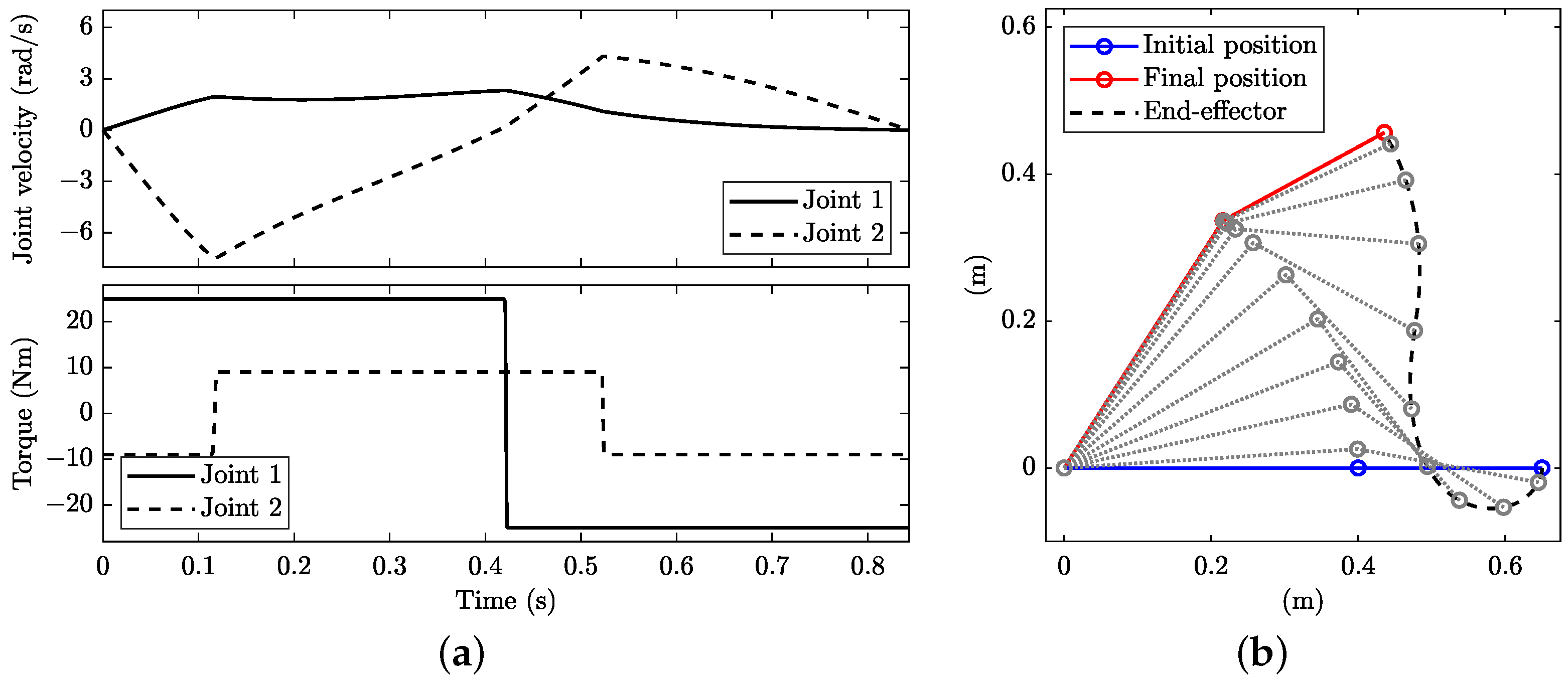
However, there are an infinite number of other minimum-time manoeuvres that are not minimum-distance in the joint space. Indeed, the bottleneck is the fastest joint, which is q 1 in this case. Therefore, the other joint, q 2 in this case, can be moved in different ways, as long as the integral of its velocity vs. time curve provides the rotation required to reach the final configuration exactly when the bottleneck joint comes to rest. As an example, Figure 4 shows a possible solution, which consists of initially actuating both joints at the limits of constraints (i.e., maximum acceleration) and then slowing down to rest joint q 2 , while joint q 1 completes the manoeuvre, always at the limits of its constraints (see Figure 4a). The path in the joint space is no longer linear; see the dashed line in Figure 3a. The path in Cartesian coordinates is shown in Figure 4b and differs from that in Figure 2b, although the manoeuvre time is identical. From a practical point of view, different numerical solutions of the OCP are related to the different guesses provided. Of course, all the numerical solutions will include the trapezoidal diagram of joint q 1 , while the diagram of joint q 2 varies.
Clearly, the solution in Figure 2 can also be obtained from an OCP whose cost consists of the distance in the q 1 vs. q 2 joint space. In such a case, the independent variable of the OCP becomes the travelled distance s (in the joint space), with the cost function being M = s f and = 0 in (2). The dynamical Equation (1) begin
q 1 = v q 1 ,
q 2 = v q 2
v q 1 = a q 1
v q 2 = a q 2
which are again related to integrator chains (with the prime—derivatives with respect to distance s—replacing the dot—derivatives with respect to time t). As regards the path constraints (3), in addition to those in (17), the following equation is added:
( q 1 ) 2 + ( q 2 ) 2 = 1
to enforce the unit magnitude of the tangent vector in the joint space, i.e., to enforce that the prime is a derivative with respect to the travelled distance s in the joint space. The numerical solution again consists of the straight line between the initial and final points. However, the manoeuvre time is not computed, since pure path planning is performed. The timing of joint motion can be computed with one of the several methods proposed in the literature once the path is provided [12].
As a final remark, the minimum-time OCP solution can be forced to select the minimum distance (in the joint space) by adding the travelled distance to the cost function, i.e.,
J = 0 t f ( 1 + w q ˙ 1 2 + q ˙ 2 2 ) d t ,
where w is a weight factor on the travelled distance term. When w = 0 , the original problem is obtained.

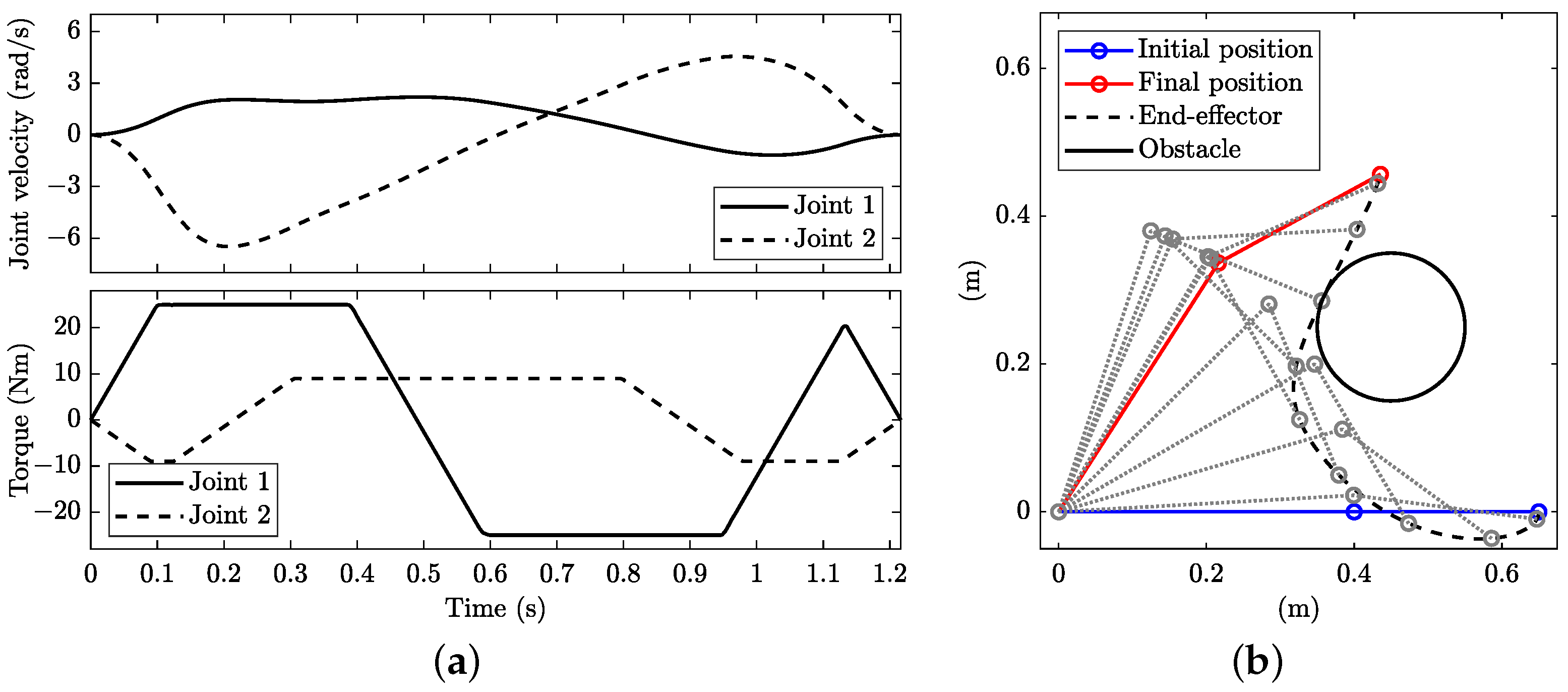
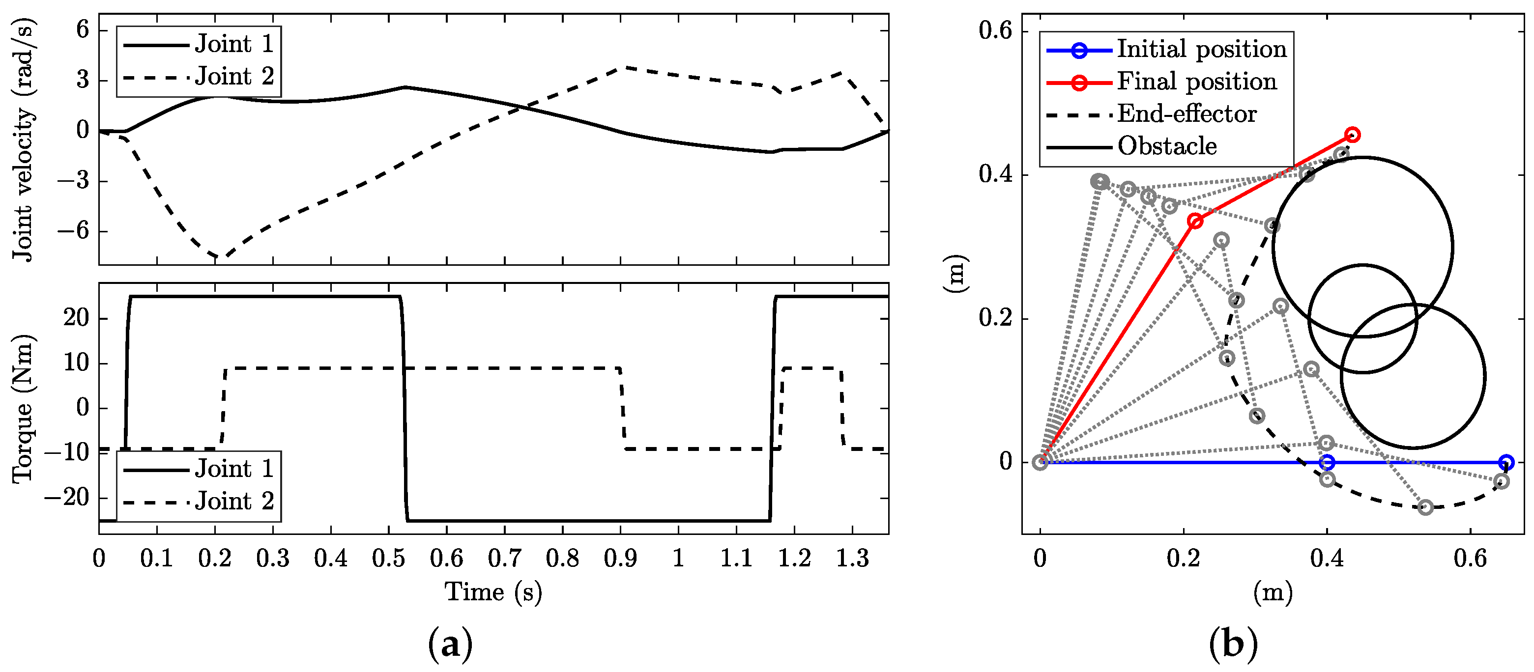
4.2. Minimum Time with Obstacle

In the case of an obstacle, the OCP can again be solved with the formulation illustrated in Section 4.1. In order to avoid multiple minimum-time solutions, cost function (32) is employed, thus forcing the solver to obtain the minimum-distance solution among the different minimum-time solutions. The only difference with respect to the OCP in Section 4.1 is in the path constraints, which need to be inflated to prevent collision with the obstacle.
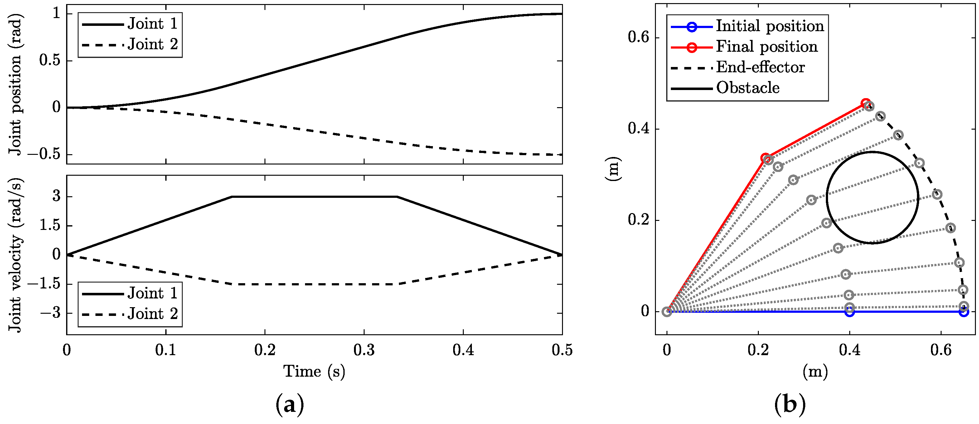
In this work, the obstacle is assumed to have a circular shape in the Cartesian space for illustration purposes. However, more complex shapes can be modelled by using multiple circular obstacles (see Section 5.4) or by employing more advanced collision techniques [42]. The constraints to avoid collisions are enforced on a discrete number of points along link 2 for illustration purposes. Of course, the constraints can potentially be enforced on link 1 as well. The additional path constraints associated with the obstacle are given by
( x P ( q ̲ , ζ ) x 0 ) 2 + ( y P ( q ̲ , ζ ) y 0 ) 2 > R 2 ζ = i N i { 1 , , N }
where N is the number of points that are monitored to prevent collision, x P and y P are from (6), and x 0 , y 0 and R are the centre coordinates and radius of the circular obstacle. In the example of the application presented in this work, the obstacle is centred at x 0 = 0.45 m, y 0 = 0.25 m with the radius r = 0.1 m (see the solid circle in Figure 5b).
The number of points N significantly affects the solution. Figure 5 shows the minimum-time solution when only the end-effector is monitored ( N = 1 ). Clearly, link 2 collides with the obstacle during motion, while the end-effector passes on the right side of the obstacle. The solution obtained in this case (Figure 5) is identical to the one obtained without the obstacle (Figure 2), again with a straight path in the joint space; see the solid line with crosses in Figure 3a. However, this solution is acceptable if the two-link manipulator is a SCARA robot and the height of the obstacle is lower than the height of link 2. On the contrary, when N = 3 points are monitored, the solution becomes the one depicted in Figure 6, with link 2 passing on the left side of the obstacle without a collision and the manoeuvre time increasing to t f = 1.180 s. The path in the joint space is no longer straight; see the dotted line in Figure 3a.

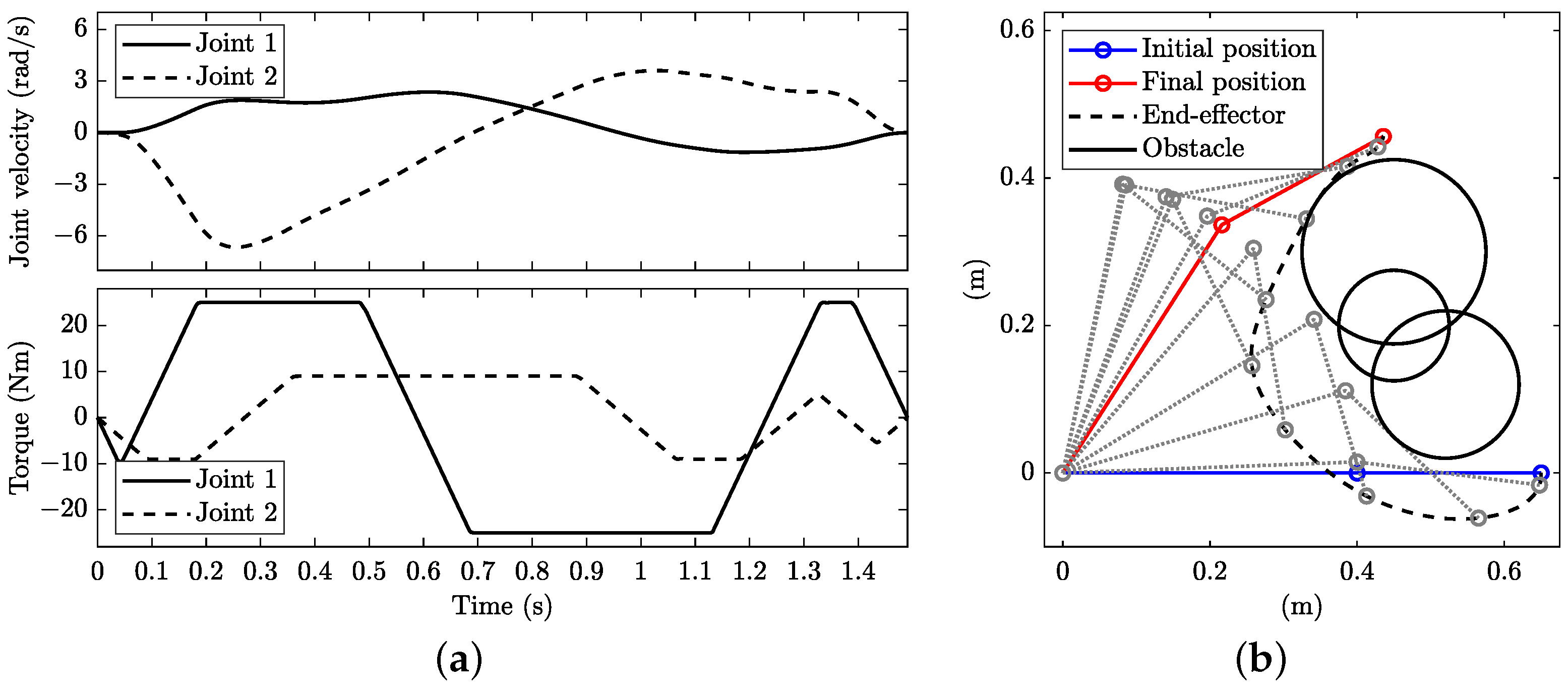
4.3. Minimum Time with Jerk Controls

The minimum-time solutions shown in Section 4.1 and Section 4.2 have discontinuities in acceleration whenever there are sudden changes in velocity, e.g., at the beginning, at the end and at the edges of the velocity profiles. Such discontinuities may lead to a number of issues in practical application but can be avoided by limiting the jerks [12]. In the OCP framework proposed, a practical solution is to control the jerks, i.e., the time derivative of acceleration, instead of the acceleration.
The dynamic equation of the OCP is inflated by including integrator chains to compute the accelerations q ̲ ¨ from the jerks q ̲ = u ̲ = { j q 1 , j q 2 } T and becomes
a ˙ q 1 = j q 1 ,
a ˙ q 2 = j q 2 ,
together with (23)–(26). The state variables are x ̲ = { q 1 , q 2 , v q 1 , v q 2 , a q 1 , a q 2 } T , while the cost function remains (32). The constraints on the velocity and acceleration are still (17) and (18), while the following bounds on the jerks are enforced:
| j q 1 | j q 1 , max , | j q 1 | j q 2 , max ,
where j q 1 , max = 500 rad/s 3 and j q 2 , max = 200 rad/s 3 are the values chosen in this work. The boundary conditions again include the initial and final positions (19) and velocities, together with zero initial and final accelerations ( q ̲ ¨ ( t i ) = q ̲ ¨ ( t f ) = 0 ); i.e., rest-to-rest manoeuvres are considered.
The minimum-time solution when including an obstacle with N = 3 points monitored to prevent collision is shown in Figure 7. The solution is quite similar to the one obtained when controlling the joint acceleration directly (Figure 6), with differences at the beginning, at the end and at the edges of the velocity profiles, where the jerks are now limited. The manoeuvre time increases to 1.286 s, which is slower than in the case of controlling the acceleration directly.

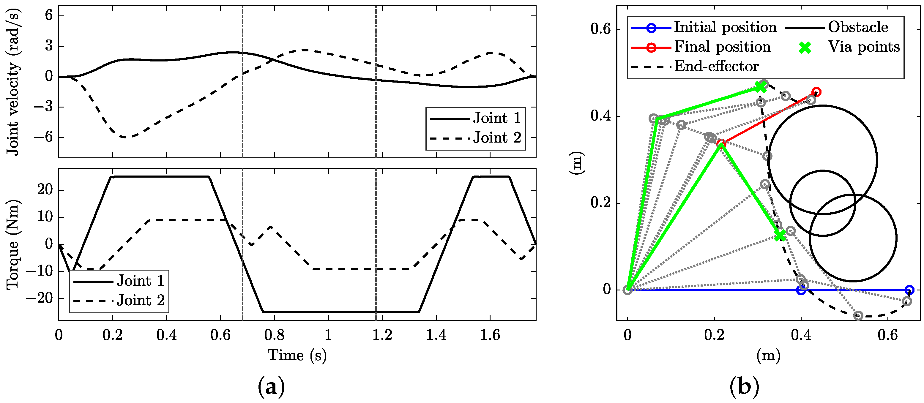
4.4. Comparison of OCP and PRM Results

In this section, the proposed OCP trajectory-planning method is compared with the PRM [32,33], which is one of the most well-known methods employed for path planning in the presence of obstacles [43]. The objective is to highlight the main differences between the approaches and optimisation results. Once the path is obtained with the PRM, polynomials can be used for motion planning. Therefore, in this case, path and motion planning are separate, in contrast to the proposed OCP approach, where the optimisation of path and motion is carried out simultaneously. The PRM is a sampling-based method that employs an algorithm to connect two points in the joint space while avoiding obstacles using randomly generated via-points within the configuration space, with the aim of minimising a defined cost. Following the approach in [43], the Dijkstra algorithm is employed in this work [32,44] to connect the points.
The configuration space is restricted within q 1 [ 0 , π / 2 ] and q 2 [ 2 3 π , 0 ] to reduce the dispersion of the randomly generated points. As in [43], the cost employed is the manoeuvre time from point h to point k, computed using
T h k = max j = 1 , 2 | q j , k q j , h | q ˙ j , max c v
where q ̲ h = { q 1 , h , q 2 , h } T and q ̲ k = { q 1 , k , q 2 , k } T are the joint positions of points h and k, respectively. The values used for the speed coefficient and maximum joint velocities are again c v = 1.5, q ˙ 1 , max = 3 rad/s and q ˙ 2 , max = 8 rad/s. The method basically consists of generating n random via-points within the configuration space, excluding the via-points inside the obstacle as well as the connections colliding with the obstacle, and running the Dijkstra algorithm with the defined cost to find sub-optimal movement between the initial and final positions. Finally, motion planning is carried out in this work using splines to connect the initial and final positions through the via-points while satisfying the velocity and acceleration limits in (17) and (18). Using splines through via-points is a standard approach [32,45,46]. In this work, for each joint, a fourth-order polynomial is used between the initial point and the first via-point, and a fourth-order polynomial is used between the last via-point and the final point, while third-order polynomials are used between the via-points. The curve resulting from such a spline, sometimes referred to as the ‘4-3-4 spline’, is C 2 , with zero initial and final velocities and accelerations, while jerks have discontinuities. The structure of the solution is thus consistent with the jerk-controlled OCP solution.
The PRM is compared with the solution obtained with the OCP in the case of an obstacle with N = 3 points monitored to prevent collision. The PRM is not deterministic; i.e., different results are obtained depending on the random points generated. Of course, changing the number of (random) points n generated also changes the solution. Therefore, in this work, the method was run with 100 different sets of randomly generated points. In addition, the number of points generated was varied between 50 and 500 with a step of 50. As a consequence, 1000 optimisations were run. The manoeuvre times obtained range between approximately 1.4 s and 4.0 s, with a mean of 2.0 s and median of 1.9 s. Figure 8 shows the PRM minimum-time solution (among the solutions found), which was obtained from a set with n = 100 randomly generated points. The Dijkstra algorithm selected four via-points (see the green crosses in Figure 8b). The manoeuvre time is 1.418 s, which is slower than that obtained with the OCP approach with jerk controls (Figure 7), although the general shapes of the velocity profiles are similar. This is not surprising, with the solution found by the PRM being sub-optimal.

5. Planning with Dynamic Constraints

Planning can also be carried out while accounting for the dynamics of the manipulator. The constraints on acceleration can be replaced with those on the joint torque:
| Q 1 | Q 1 , max | Q 2 | Q 2 , max ,
where Q 1 , max = 25 Nm and Q 2 , max = 9 Nm are the values chosen in this work (again from [25]). However, the kinematic constraints on the velocity (17) still hold, as well as the boundary condition on the initial and final positions (19) and velocities.
The controls are torque u ̲ = { Q 1 , Q 2 } T (instead of the acceleration used in Section 4), while the states remains the same, i.e., x ̲ = { q 1 , q 2 , v q 1 , v q 2 } . The dynamic equations consist of the integrator chains and the equation of motion (in Section 4, only the integrator chains were used).
q ˙ 1 = v q 1 ,
q ˙ 2 = v q 2 ,
v ˙ q 1 v ˙ q 2 = M 1 ( Q ̲ c ( q ̲ , q ˙ ̲ ) ) ,
where (41) is from (11). The cost function of the minimum-time OCP remains the one used in Section 4.1, i.e., M = 0 and = 1 in (2), with time t as the independent variable.

5.1. Minimum Time

The solution is illustrated in Figure 9, which shows that the control of both joints is bang–bang (bottom plot of Figure 9a) and none of the joints is engaged at its maximum velocity (top plot of Figure 9a). The optimal solution is quite different from that obtained with the kinematic constraints only, which is also evident when comparing the Cartesian plots in Figure 9b (solution with dynamic constraints) with Figure 2b (solution with kinematic constraints). The path in the joint space is thus not straight; see the solid line in Figure 3b. The manoeuvre time is t f = 1.002 s, which is slower than in the case with kinematic constraints, although with joint accelerations that are locally up to 18 rad/s 2 (on q 1 ) and 59 rad/s 2 (on q 2 ), i.e., much larger than those enforced in the OCP with kinematic constraints.
When repeating the OCP optimisation while enforcing q 1 and q 2 to follow the minimum-distance path in the joint space (see dashed line in Figure 3b), the manoeuvre time rises to t f = 1.081 s, which confirms that this solution is not optimal when including dynamic constraints associated with equations of motion. The optimal solution becomes bang–bang in the fastest joint only (Figure 10), while it is bang–bang in both joints in Figure 9. The maximum accelerations are 3.5 rad/s 2 and 1.8 rad/s 2 for joints q 1 and q 2 , respectively. Of course, the same solution can be obtained while enforcing such maximum accelerations in the OCP of Section 4.
When comparing the control structures in Figure 9 and Figure 10, it can be observed that they differ in the number of bangs: in the former, there are two bangs in q 1 and three in q 2 , and in the latter, there are two bangs in q 1 , while in q 2 , the control is such that the pre-defined path is followed, which results in an almost bang–bang solution.
If the payload M is neglected, the solution becomes the one illustrated in Figure 11. As expected, the manoeuvre time is reduced to t f = 0.843 s, since the same maximum torques now move a system with a reduced mass. The maximum accelerations reached by joints q 1 and q 2 are 18 rad/s 2 and 69 rad/s 2 , respectively.
Again, when repeating optimisation while enforcing q 1 and q 2 to follow the minimum-distance path in the joint space, the manoeuvre time rises to t f = 0.921 s. The maximum accelerations are 4.8 rad/s 2 (joint 1) and 2.4 rad/s 2 (joint 2).

5.2. Minimum Time with Obstacle

When an obstacle is considered, the approach in Section 4.2 is again employed: i.e., the path constraints are inflated with the obstacle equations in (33). When preventing the collision on the end-effector only (i.e., N = 1 ), the optimal solution is the one in Figure 12, which is different from the solution obtained when neglecting the obstacle (Figure 9). This was not the case for the OCP with kinematic constraints, where the solutions without an obstacle and with an obstacle N = 1 coincide. The path in the joint space is not straight; see the dash-dotted line in Figure 3b. The manoeuvre time with N = 1 is t f = 1.046 s, which is slightly slower than the case without the obstacle. However, in this solution, there is a clear collision between several points of link 2 and the obstacle, unless the two-link manipulator is a SCARA robot and the height of the obstacle is lower than the height of link 2.
The collision is prevented when monitoring N = 3 points of link 2. The manoeuvre time rises to t f = 1.098 s. The solution is shown in Figure 13. In contrast to the case with N = 1 , the end-effector passes on the left side of the obstacle, again with a non-straight path; see the dotted line in Figure 3b. The control structures in Figure 12 and Figure 13 differ in the number of bangs: in the former, there are two bangs in q 1 and five in q 2 , while in the latter, there are three bangs in q 1 and three in q 2 .

5.3. Limitations on the Torque Rate of Change

The minimum-time solutions obtained in Section 5.1 and Section 5.2 are characterised by a bang–bang control structure, which may cause a number of well-known issues in practical applications. Such discontinuities can be avoided when using the rate of change in torque as the control variable instead of the torque. The dynamic equations of the OCP are further inflated by including the integrator chains related to the rates of change J 1 and J 2 in torque and become
Q ˙ 1 = J 1 ,
Q ˙ 2 = J 2 ,
together with (39)–(41).
The state variables become x ̲ = { q 1 , q 2 , v q 1 , v q 2 , Q 1 , Q 2 } T , the control variables become u ̲ = { J 1 , J 2 } T , and the cost function remains the same, i.e., the manoeuvre time. The constraints on velocity and torque are still (17) and (38), while the following bounds on the rates of change in torque are introduced:
| J 1 | J 1 , max , | J 2 | J 2 , max ,
where J 1 , max = 250 Nm/s and J 2 , max = 100 Nm/s are the values chosen in this work (estimated from [25]). The boundary conditions again include the initial and final positions (19) and velocities, together with zero initial and final joint torques ( Q ̲ ( t i ) = Q ̲ ( t f ) = 0 ); i.e., rest-to-rest manoeuvres are considered.
The solution without an obstacle is illustrated in Figure 14. The solution is quite similar to that obtained when directly controlling the joint torque instead of the rate of change (see Figure 9), with evident differences at the beginning, at the end and at the bangs, where the torques vary in the maximum rate of change (bottom plot in Figure 14a). Therefore, the velocity profiles (top plot in Figure 14a) become smoother and start and end with zero acceleration. The manoeuvre time increases to t f = 1.106 s, which is slower than in the case of controlling the joint torque directly.
When including an obstacle with N = 3 using the same approach employed in Section 4.2, the solution becomes the one shown in Figure 15. The manoeuvre time rises to 1.216 s. Again, the torques vary in the maximum rate of change (bottom plot in Figure 14a) at the beginning, at the end and at the bangs of the torque-controlled solution (see Figure 13), resulting in smoother velocity profiles (top plot in Figure 14a).

5.4. Multiple Obstacles

The approach proposed in Section 4.2 can be employed for obstacles having complex shapes, which are modelled by a combination of circular obstacles. The associated path constraints become
( x P ( q ̲ , ζ ) x 0 j ) 2 + ( y P ( q ̲ , ζ ) y 0 j ) 2 < R j 2 ζ = i N i { 1 , , N } j { 1 , , C } ,
where C is the number of circular obstacles. As an example application, an obstacle modelled by three intersecting circular obstacles is considered in this work. The three obstacles are centred at x 01 = 0.52 m, y 01 = 0.12 m, x 02 = 0.45 m, y 02 = 0.2 m and x 03 = 0.45 m, y 03 = 0.3 m, with radii R 1 = 0.1 m, R 2 = 0.075 m and R 3 = 0.125 m, respectively; see the solid circles in Figure 16b.
Figure 16 shows the minimum-time solution with N = 3 points monitored to prevent collision when controlling the joint torque directly, i.e., without a limitation on its rate of change. The manoeuvre time is 1.362 s. The control structure (bottom plot in Figure 16a) is again bang–bang, with four bangs for q 1 and five bangs for q 2 . When limiting the rate of change in the joint torque, the solution becomes the one depicted in Figure 17. The manoeuvre time increases to 1.491 s. Again, the torques vary in the maximum rate of change (bottom plot in Figure 17a), with smoother velocity profiles as compared to the solution obtained when controlling the torque directly (see top plots in Figure 16a and Figure 17a). When increasing the number of points monitored to prevent collision to N = 10 , the solution remains the same, in this example.

5.5. Via-Point Constraints

Although the proposed approach does not require the provision of a path, with the path being a result of optimisation, via-points can be added to the problem. In such a case, the OCP finds the optimal path (and corresponding joint motion) that minimises the manoeuvre time while passing through V pre-defined via-points. Additional constraints related to the via-points are thus added to the problem in Section 2. In particular, the OCP is divided into V + 1 phases. The first phase is from the initial configuration to the first via-point, and the last phase is from the last via-point to the final configuration, while the intermediate phases are between the different via-points. The OCP consists of solving all the phases simultaneously. The via-point constraint is enforced using
q ̲ ( t f , v ) = q ̲ v v { 1 , , V } ,
where q ( t f , v ) is the joint position at the end of phase v (i.e., at the final time t f , v of phase v), while q ̲ v is the via-point expressed in terms of the joint positions. Of course, the via-point can alternatively be given in terms of Cartesian coordinates, from which the joint coordinates are obtained from inverse kinematics.
The following additional boundary conditions also need to be added in order to enforce continuity between the phases:
x ̲ ( t f , v ) = x ̲ ( t i , v + 1 ) , t f , v = t i , v + 1 , v { 1 , , V } ,
where x ̲ ( t f , v ) is the state at the end of phase v (i.e., at the final time t f , v of phase v), while x ̲ ( t i , v + 1 ) is the state at the beginning of phase v + 1 (i.e., at the initial time t i , v + 1 of phase v + 1 ). The switching times between the phases and the joint velocities at the via-points are not pre-defined and thus are a result of optimisation.
As an example application, two via-points at q ̲ 1 = { 1.0 , 2.0 } T and q ̲ 2 = { 1.4 , 1.1 } T are considered in this work; see the green crosses in Figure 18b. The solution with a limitation on the rate of change in the joint torque and three obstacles is depicted in Figure 18. The manoeuvre time is 1.771 s, which is slower than the corresponding solution without via-points (Figure 17). The switching times between the phases are 0.682 s (first via-point) and 1.177 s (second via-point). When comparing the solution with via-points with the one without via-points, it can be observed that the torque on q 1 is not significantly affected, with the pattern remaining characterised by a ‘min-max-min-max’ pattern. On the contrary, the torque on q 2 gains a ‘min-max’ on top of the original ‘min-max-min-max-min’ pattern. Of course, the lengths of the constant torque sections also vary.

5.6. Redundant Manipulator

A four-link planar manipulator is considered in this section to show the ‘scalability’ of the approach to more complex robots. The system has four degrees of freedom (with q ̲ = { q 1 , q 2 , q 3 , q 4 } T being the relative angles between the links; see Figure 19) and is redundant, since two degrees of freedom would be sufficient to track the target Cartesian position (as long as this is within the workspace). The manipulator is obtained from the baseline manipulator in Section 3 by splitting the two links. The centre of mass and inertia resulting from the two arms obtained by splitting baseline link 1 are identical (when q 2 = 0 ) to the corresponding values of baseline link 1. Similarly, the centre of mass and inertia resulting from the two arms obtained by splitting baseline link 2 are identical (when q 4 = 0 ) to the corresponding values of baseline link 2. The equations of motion can be obtained following the same approach presented in Section 3, where the kinetic energy begins
T = 1 2 m 1 | v ̲ G 1 | 2 + 1 2 I 1 q ˙ 1 2 + 1 2 m 2 | v ̲ G 2 | 2 + 1 2 I 2 ( q ˙ 1 + q ˙ 2 ) 2 + 1 2 m 3 | v ̲ G 3 | 2 + + 1 2 I 3 ( q ˙ 1 + q ˙ 2 + q ˙ 3 ) 2 + 1 2 m 4 | v ̲ G 4 | 2 + 1 2 I 4 ( q ˙ 1 + q ˙ 2 + q ˙ 3 + q ˙ 4 ) 2 + 1 2 M | v ̲ P 4 | 2 ,
while the torques applied to the links are
Q ̲ = { Q 1 , Q 2 , Q 3 , Q 4 } T .
The resulting equations of motion can again be written in the form of (11), where M is now a 4 × 4 matrix and c ̲ is a 4 × 1 vector. However, they are not reported for the conciseness of presentation.
The rate of change J ̲ = { J 1 , J 2 , J 3 , J 4 } T in the four actuator torques of the manipulator are controlled, as in Section 5.3, to avoid bang–bang in the torques. Joint motions are limited in their maximum velocities by
| q ˙ 1 | q ˙ 1 , max | q ˙ 2 | q ˙ 2 , max | q ˙ 3 | q ˙ 3 , max | q ˙ 4 | q ˙ 4 , max
where q ˙ 1 , max = q ˙ 2 , max = 3 rad/s and q ˙ 3 , max = q ˙ 4 , max = 8 rad/s are the values chosen in this work. The constraints on the joint torques are
| Q 1 | Q 1 , max | Q 2 | Q 2 , max | Q 3 | Q 3 , max | Q 4 | Q 4 , max
with Q 1 , max = 25 Nm, Q 2 , max =15 Nm, Q 3 , max = 9 Nm and Q 4 , max = 5 Nm, while the bounds on the rate of change in torque are
| J 1 | J 1 , max | J 2 | J 2 , max | J 3 | J 3 , max | J 4 | J 4 , max
where J 1 , max = 250 Nm/s, J 2 , max = 150 Nm/s, J 3 , max = 100 Nm/s and J 4 , max = 50 Nm/s are the values chosen in this work. The initial and final positions of the joints are
q ̲ ( t i ) = { q 1 i , q 2 i , q 3 i , q 4 i } T q ̲ ( t f ) = { q 1 f , q 2 f , q 3 f , q 4 f } T .
where q 1 i = q 2 i = q 3 i = q 4 i = 0 and q 1 f = 1 rad, q 3 f = −0.5 rad and q 2 f = q 4 f = 0 ; i.e., links 1 and 2 are aligned at the beginning and the end with baseline link 1, while links 3 and 4 are aligned at the beginning and the end with baseline link 2. The constraints to avoid collisions are enforced on links 2, 3 and 4 on N points along each link.
In sum, the OCP has 12 state variables (i.e., q ̲ , q ̲ ˙ , Q ̲ ) and 4 control variables (i.e., J ̲ ), with the cost function (2) being the manoeuvre time. The dynamic equations (1) consist of integration chains and manipulator equations of motion, and the path constraints (3) consist of (50) and (51) plus constraints related to collision avoidance. The boundary conditions (4) consist of (53), while the bounds on inputs (19) are (52).
Figure 20 shows the minimum-time solution with three circular obstacles, as in Section 5.4, and N = 2 points monitored to prevent collision along each link. The manoeuvre time is 1.029 s, which is faster than in then case of the two-link manipulator (Figure 17). This is not surprising, since the redundancies are leveraged to improve the performance.

6. Remarks

All the optimisations performed in this work start with a mesh consisting of 50 equally spaced intervals with 4 collocation points for each mesh interval. When obstacles are included, special attention is paid to providing the solver with an almost feasible guess solution, i.e., that which (almost) does not collide with the obstacles. The proposed method converges to an optimal solution, although (like most optimisation approaches) there is no guarantee that the solution found is locally optimal or globally optimal. Multiple guess solutions have been employed to confirm the optimality of the solutions reported in this work.
Problem scaling can significantly affect the convergence of the optimisation algorithm. Indeed, convergence criteria are often based on the notation of ‘small’ and ‘large’. A typical approach is to scale the problem variables from their physical representation to dimensionless quantities, which have desirable properties from the numerical perspective. In this work, all problem variables are scaled according to a reference mass m 0 = m 1 + m 2 + M , a reference length l 0 = l 1 + l 2 and a reference angular acceleration q ¨ 0 = max ( q ¨ 1 , max , q ¨ 2 , max ) for planning with kinematic constraints or according to a reference torque Q 0 = max ( Q 1 max , Q 2 max ) for planning with dynamic constraints. Hence, the scaling of time is 1 / q ¨ 0 and m 0 l 0 2 / Q 0 for optimisation with kinematic and dynamic constraints, respectively.
The solution is typically found after 2–5 mesh refinements, with a mesh tolerance in GPOPS-II of 10 5 and an error for the IPOPT solver of 10 7 . The computational cost of the planning problems can be assessed considering the number of equations and the CPU time. In the case of planning with kinematic constraints, the OCPs consist of around 1000–1600 equations with CPU times ranging within 1–2 s (on a standard PC with Intel i7 and 16 GB RAM), depending on the obstacle and the number of points that are monitored to prevent collision. In the case of planning with dynamic constraints, the number of equations to solve is 1000–5000, with CPU times rising to 2–30 s. Of course, large CPU times are associated with problems involving multiple obstacles, via-point constraints and/or more complex robots. The number of points N monitored to prevent collision obviously affects the solution time. As an example, with N = 10 , the solution times are typically 50% larger than in the case with N = 3 .

7. Conclusions

In this work, the trajectory-planning problem is tackled with a nonlinear optimal control approach, which requires neither the path nor the control structure to be defined. The approach is demonstrated on a two-link manipulator for illustration purposes. The focus is on minimum-time manoeuvring, which is solved by using both kinematic and dynamic constraints, both without and with obstacles. Some classic results were obtained, such as the trapezoidal pattern of the joint velocity—which provides a minimum-time and minimum-distance (in the space of the joint coordinates) solution of the unconstrained rest-to-rest problem—and the bang–bang pattern of the control torques. Either the jerk control or the control of the rate of change in torque is used to remove the discontinuities of the bang–bang solutions. The approach is demonstrated to also be capable of efficiently performing planning when obstacles are included, without the need to provide via-points. However, a number of via-points can also be included in the optimisation, while the path between the via-points need not be defined. The effect of the number of collision constraints employed is also shown. The presented approach is suitable for application to different manipulators as well. The results obtained with the proposed approach are also compared with those of the standard Probabilistic Roadmap Method (PRM), confirming that the PRM solution is sub-optimal relative to the OCP solution. The ‘scalability’ to more complex scenarios is also shown by applying the approach to a redundant four-degree-of-freedom manipulator.

Author Contributions

Conceptualisation, M.M. and G.R.; methodology, M.M., S.L. and M.B.; software, S.L.; validation, M.M. and S.L.; formal analysis, S.L.; investigation, M.M. and S.L.; writing—original draft preparation, M.M. and S.L.; writing—review and editing, M.M., S.L., M.B. and G.R.; visualisation, S.L.; supervision M.M. and G.R. All authors have read and agreed to the published version of the manuscript.

Funding

This work was partially supported by a Ph.D. grant funded by Fondo per lo Sviluppo e la Coesione (FSC), within the Piano Stralcio ‘Ricerca e innovazione 2015–2017’.

Institutional Review Board Statement

Not applicable.

Informed Consent Statement

Not applicable.

Data Availability Statement

Not applicable.

Conflicts of Interest

The authors declare no conflict of interest.

References

  1. Carlberg, M.; Kreutzer, S.; Smit, J.; Moeller, C. Industry 4.0; DG for Internal Policies of the Union; European Parliament: Strasbourg, France, 2016. [Google Scholar]
  2. Xu, L.D.; Xu, E.L.; Li, L. Industry 4.0: State of the art and future trends. Int. J. Prod. Res. 2018, 56, 2941–2962. [Google Scholar] [CrossRef]
  3. Goel, R.; Gupta, P. Robotics and industry 4.0. In A Roadmap to Industry 4.0: Smart Production, Sharp Business and Sustainable Development; Springer: Berlin/Heidelberg, Germany, 2020; pp. 157–169. [Google Scholar]
  4. Bobrow, J.; Dubowsky, S.; Gibson, J. Time-Optimal Control of Robotic Manipulators Along Specified Paths. Int. J. Robot. Res. 1985, 4, 3–17. [Google Scholar] [CrossRef]
  5. Shin, K.; McKay, N. Minimum-time control of robotic manipulators with geometric path constraints. IEEE Trans. Autom. Control 1985, 30, 531–541. [Google Scholar] [CrossRef]
  6. Pfeiffer, F.; Johanni, R. A concept for manipulator trajectory planning. IEEE J. Robot. Autom. 1987, 3, 115–123. [Google Scholar] [CrossRef]
  7. Kim, J.; Kim, S.; Kim, S.; Kim, D. A practical approach for minimum-time trajectory planning for industrial robots. Ind. Robot Int. J. 2010, 37, 51–61. [Google Scholar] [CrossRef]
  8. Barre, P.J.; Bearee, R.; Borne, P.; Dumetz, E. Influence of a jerk controlled movement law on the vibratory behaviour of high-dynamics systems. J. Intell. Robot. Syst. 2005, 42, 275–293. [Google Scholar] [CrossRef]
  9. Zanotto, V.; Gasparetto, A.; Lanzutti, A.; Boscariol, P.; Vidoni, R. Experimental Validation of Minimum Time-jerk Algorithms for Industrial Robots. J. Intell. Robot. Syst. 2011, 64, 197–219. [Google Scholar] [CrossRef]
  10. Field, G.; Stepanenko, Y. Iterative dynamic programming: An approach to minimum energy trajectory planning for robotic manipulators. In Proceedings of the IEEE International Conference on Robotics and Automation, Minneapolis, MN, USA, 22–28 April 1996; Volume 3, pp. 2755–2760. [Google Scholar] [CrossRef]
  11. Boscariol, P.; Caracciolo, R.; Richiedei, D.; Trevisani, A. Energy Optimization of Functionally Redundant Robots through Motion Design. Appl. Sci. 2020, 10, 3022. [Google Scholar] [CrossRef]
  12. Gasparetto, A.; Boscariol, P.; Lanzutti, A.; Vidoni, R. Path Planning and Trajectory Planning Algorithms: A General Overview. In Motion and Operation Planning of Robotic Systems: Background and Practical Approaches; Carbone, G., Gomez-Bravo, F., Eds.; Springer International Publishing: Cham, Switzerland, 2015; pp. 3–27. [Google Scholar] [CrossRef]
  13. Zhang, Q.; Zhao, M.Y. Minimum time path planning of robotic manipulator in drilling/spot welding tasks. J. Comput. Des. Eng. 2016, 3, 132–139. [Google Scholar] [CrossRef]
  14. Lovato, S.; Massaro, M. Three-dimensional fixed-trajectory approaches to the minimum-lap time of road vehicles. Veh. Syst. Dyn. 2022, 60, 3650–3667. [Google Scholar] [CrossRef]
  15. Massaro, M.; Limebeer, D.J.N. Minimum-lap-time optimisation and simulation. Veh. Syst. Dyn. 2021, 59, 1069–1113. [Google Scholar] [CrossRef]
  16. Lovato, S.; Massaro, M. A three-dimensional free-trajectory quasi-steady-state optimal-control method for minimum-lap-time of race vehicles. Veh. Syst. Dyn. 2022, 60, 1512–1530. [Google Scholar] [CrossRef]
  17. Gilbert, E.; Johnson, D. Distance functions and their application to robot path planning in the presence of obstacles. IEEE J. Robot. Autom. 1985, 1, 21–30. [Google Scholar] [CrossRef]
  18. Bobrow, J. Optimal robot plant planning using the minimum-time criterion. IEEE J. Robot. Autom. 1988, 4, 443–450. [Google Scholar] [CrossRef]
  19. Meier, E.B.; Bryson, A.E., Jr. Efficient algorithm for time-optimal control of a two-link manipulator. J. Guid. Control Dyn. 1990, 13, 859–866. [Google Scholar] [CrossRef]
  20. Shiller, Z.; Dubowsky, S. On computing the global time-optimal motions of robotic manipulators in the presence of obstacles. IEEE Trans. Robot. Autom. 1991, 7, 785–797. [Google Scholar] [CrossRef]
  21. Shiller, Z.; Lu, H.H. Computation of Path Constrained Time Optimal Motions With Dynamic Singularities. J. Dyn. Syst. Meas. Control 1992, 114, 34–40. [Google Scholar] [CrossRef]
  22. Massaro, M.; Lovato, S.; Limebeer, D.J.N. The Optimal Erection of the Inverted Pendulum. Appl. Sci. 2022, 12, 8112. [Google Scholar] [CrossRef]
  23. Szyszkowski, W.; Fotouhi-C, R. Improving time-optimal maneuvers of two-link robotic manipulators. J. Guid. Control Dyn. 2000, 23, 888–889. [Google Scholar] [CrossRef]
  24. An, Z.; Wu, H.; Shi, D. Minimum-time optimal control of robotic manipulators based on Hamel’s integrators. Meccanica 2019, 54, 2521–2537. [Google Scholar] [CrossRef]
  25. Ghasemi, M.H.; Kashiri, N.; Dardel, M. Time-optimal trajectory planning of robot manipulators in point-to-point motion using an indirect method. Proc. Inst. Mech. Eng. Part C J. Mech. Eng. Sci. 2012, 226, 473–484. [Google Scholar] [CrossRef]
  26. Bertolazzi, E.; Biral, F.; Da Lio, M. real-time motion planning for multibody systems. Multibody Syst. Dyn. 2007, 17, 119–139. [Google Scholar] [CrossRef]
  27. Lovato, S.; Massaro, M.; Limebeer, D.J.N. Curved-ribbon-based track modelling for minimum lap-time optimisation. Meccanica 2021, 56, 2139–2152. [Google Scholar] [CrossRef]
  28. Limebeer, D.J.N.; Massaro, M. Dynamics and Optimal Control of Road Vehicles; Oxford University Press: Oxford, UK, 2018. [Google Scholar] [CrossRef]
  29. Liu, F.; Hager, W.W.; Rao, A.V. Adaptive mesh refinement method for optimal control using decay rates of Legendre polynomial coefficients. IEEE Trans. Control Syst. Technol. 2017, 26, 1475–1483. [Google Scholar] [CrossRef]
  30. Liu, F.; Hager, W.W.; Rao, A.V. Adaptive mesh refinement method for optimal control using nonsmoothness detection and mesh size reduction. J. Frankl. Inst. 2015, 352, 4081–4106. [Google Scholar] [CrossRef]
  31. Weinstein, M.J.; Rao, A.V. Algorithm 984: ADiGator, a toolbox for the algorithmic differentiation of mathematical functions in MATLAB using source transformation via operator overloading. ACM Trans. Math. Softw. 2017, 44, 1–25. [Google Scholar] [CrossRef]
  32. LaValle, S.M. Planning Algorithms; Cambridge University Press: Cambridge, UK, 2006. [Google Scholar]
  33. Kavraki, L.; Svestka, P.; Latombe, J.C.; Overmars, M. Probabilistic roadmaps for path planning in high-dimensional configuration spaces. IEEE Trans. Robot. Autom. 1996, 12, 566–580. [Google Scholar] [CrossRef]
  34. Betts, J.T. Practical Methods for Optimal Control and Estimation Using Nonlinear Programming, 2nd ed.; Society for Industrial and Applied Mathematics: Philadelphia, PA, USA, 2010. [Google Scholar] [CrossRef]
  35. Dal Bianco, N.; Biral, F.; Bertolazzi, E.; Massaro, M. Comparison of Direct and Indirect Methods for Minimum Lap Time Optimal Control Problems. Veh. Syst. Dyn. 2018, 57, 665–696. [Google Scholar] [CrossRef]
  36. Patterson, M.A.; Rao, A.V. GPOPS - II: A Matlab Software for Solving Multiple-Phase Optimal Control Problems Using hp–Adaptive Gaussian Quadrature Collocation Methods and Sparse Nonlinear Programming. ACM Trans. Math. Softw. 2014, 41, 1–37. [Google Scholar] [CrossRef]
  37. Wächter, A.; Biegler, L.T. On the Implementation of an Interior-Point Filter Line-Search Algorithm for Large-Scale Nonlinear Programming. Math. Program. 2006, 106, 25–57. [Google Scholar] [CrossRef]
  38. Squire, W.; Trapp, G. Using Complex Variables to Estimate Derivatives of Real Functions. SIAM Rev. 1998, 40, 110–112. [Google Scholar] [CrossRef]
  39. Martins, J.R.R.A.; Sturdza, P.; Alonso, J.J. The Connection Between the Complex-Step Derivative Approximation and Algorithmic Differentiation. AIAA Paper. In Proceedings of the 39th Aerospace Sciences Meeting and Exhibit, Atlanta, GA, USA, 8–11 January 2001. [Google Scholar]
  40. Martins, J.R.R.A.; Sturdza, P.; Alonso, J.J. The Complex-Step Derivative Approximation. ACM Trans. Math. Softw. 2003, 29, 245–262. [Google Scholar] [CrossRef]
  41. Biagiotti, L.; Melchiorri, C. Trajectory Planning for Automatic Machines and Robots; Springer Science & Business Media: Cham, Switzerland, 2008. [Google Scholar]
  42. Bottin, M.; Boschetti, G.; Rosati, G. A novel collision avoidance method for serial robots. Mech. Mach. Sci. 2019, 66, 293–301. [Google Scholar] [CrossRef]
  43. Bottin, M.; Rosati, G. Trajectory optimization of a redundant serial robot using cartesian via points and kinematic decoupling. Robotics 2019, 8, 101. [Google Scholar] [CrossRef]
  44. Dijkstra, E.W. A Note on Two Problems in Connexion with Graphs. Numer. Math. 1959, 1, 269–271. [Google Scholar] [CrossRef]
  45. Jazar, R.N. Theory of Applied Robotics, 3rd ed.; Springer: Berlin/Heidelberg, Germany, 2022. [Google Scholar]
  46. Siciliano, B.; Sciavicco, L.; Villani, L.; Oriolo, G. Robotics: Modelling, Planning and Control; Springer Publishing Company, Incorporated: Berlin/Heidelberg, Germany, 2010. [Google Scholar]
Figure 1. Two-link planar manipulator model.
Robotics 12 00064 g001
Figure 2. Minimum-time and minimum-distance planning with kinematic constraints: (a) joint angular positions (top) and velocities (bottom) and (b) stroboscopic movie of the manipulator with 10 equally spaced time steps.
Robotics 12 00064 g002
Figure 3. Path in the joint space ( q 1 vs. q 2 diagram) for planning with (a) kinematic constraints and (b) dynamic constraints. The blue circle and red square denote the initial and final positions, respectively.
Robotics 12 00064 g003
Figure 4. Minimum-time but no minimum-distance planning with kinematic constraints: (a) joint angular position (top) and velocities (bottom) and (b) stroboscopic movie of the manipulator with 10 equally spaced time steps.
Robotics 12 00064 g004
Figure 5. Minimum-time planning with kinematic constraints including an obstacle with N = 1 : (a) joint angular position (top) and velocities (bottom) and (b) stroboscopic movie of the manipulator with 10 equally spaced time steps.
Robotics 12 00064 g005
Figure 6. Minimum-time planning with kinematic constraints including an obstacle with N = 3 : (a) joint angular position (top) and velocities (bottom) and (b) stroboscopic movie of the manipulator with 10 equally spaced time steps.
Robotics 12 00064 g006
Figure 7. Minimum-time planning with kinematic constraints and limitation of the joint jerks including an obstacle with N = 3 : (a) joint angular position (top) and velocities (bottom) and (b) stroboscopic movie of the manipulator with 10 equally spaced time steps.
Robotics 12 00064 g007
Figure 8. Minimum-time planning using PRM including an obstacle with N = 3 : (a) joint angular position (top) and velocities (bottom) and (b) stroboscopic movie of the manipulator with 10 equally spaced time steps.
Robotics 12 00064 g008
Figure 9. Minimum-time planning with dynamic constraints: (a) joint angular velocity (top) and torque (bottom) and (b) stroboscopic movie of the manipulator with 10 equally spaced time steps.
Robotics 12 00064 g009
Figure 10. Minimum-time planning with dynamic constraints and minimum-distance (in the joint space) constraint: (a) joint angular velocity (top) and torque (bottom), and (b) stroboscopic movie of the manipulator with 10 equally spaced time steps.
Robotics 12 00064 g010
Figure 11. Minimum-time planning with dynamic constraints and no payload: (a) joint angular velocity (top) and torque (bottom) and (b) stroboscopic movie of the manipulator with 10 equally spaced time steps.
Robotics 12 00064 g011
Figure 12. Minimum-time planning with dynamic constraints and obstacle with N = 1 : (a) joint angular velocity (top) and torque (bottom) and (b) stroboscopic movie of the manipulator with 10 equally spaced time steps.
Robotics 12 00064 g012
Figure 13. Minimum-time planning with dynamic constraints and obstacle with N = 3 : (a) joint angular velocity (top) and torque (bottom) and (b) stroboscopic movie of the manipulator with 10 equally spaced time steps.
Robotics 12 00064 g013
Figure 14. Minimum-time planning with dynamic constraints and limitation on the rate of change in torque: (a) joint angular velocity (top) and torque (bottom) and (b) stroboscopic movie of the manipulator with 10 equally spaced time steps.
Robotics 12 00064 g014
Figure 15. Minimum-time planning with dynamic constraints and limitation on the rate of change in torque in the presence of obstacle with N = 3 : (a) joint angular velocity (top) and torque (bottom) and (b) stroboscopic movie of the manipulator with 10 equally spaced time steps.
Robotics 12 00064 g015
Figure 16. Minimum-time planning with dynamic constraints and multiple obstacles with N = 3 : (a) joint angular velocity (top) and torque (bottom) and (b) stroboscopic movie of the manipulator with 10 equally spaced time steps.
Robotics 12 00064 g016
Figure 17. Minimum-time planning with dynamic constraints and limitation on the rate of change in the joint torque in the presence of multiple obstacles with N = 3 : (a) joint angular velocity (top) and torque (bottom) and (b) stroboscopic movie of the manipulator with 10 equally spaced time steps.
Robotics 12 00064 g017
Figure 18. Minimum-time planning with dynamic constraints and via-point constraint: (a) joint angular velocity (top) and torque (bottom) and (b) stroboscopic movie of the manipulator with 10 equally spaced time steps. In (a), the vertical dash-dotted lines denote the switching time between the phases.
Robotics 12 00064 g018
Figure 19. Four-link planar manipulator model ( q 3 and q 4 are negative in the configuration depicted).
Robotics 12 00064 g019
Figure 20. Minimum-time planning with dynamic constraints for a four-link planar redundant manipulator: (a) joint angular velocity (top) and torque (bottom) and (b) stroboscopic movie of the manipulator with 10 equally spaced time steps.
Robotics 12 00064 g020
Table 1. Two-link planar manipulator dataset.
SymbolDescriptionValue
l 1 Length of link 10.4 m
l 2 Length of link 20.25 m
m 1 Mass of link 129.58 kg
m 2 Mass of link 215 kg
I 1 Moment of inertia of link 1 (with respect to the centre of mass)0.417 kgm 2
I 2 Moment of inertia of link 2 (with respect to the centre of mass)0.206 kgm 2
( b 1 , h 1 ) Position of the centre of mass of link 1 ( l 1 / 2 , 0 )
( b 2 , h 2 ) Position of the centre of mass of link 2 ( l 2 / 2 , 0 )
MMass of the payload6 kg
Disclaimer/Publisher’s Note: The statements, opinions and data contained in all publications are solely those of the individual author(s) and contributor(s) and not of MDPI and/or the editor(s). MDPI and/or the editor(s) disclaim responsibility for any injury to people or property resulting from any ideas, methods, instructions or products referred to in the content.

