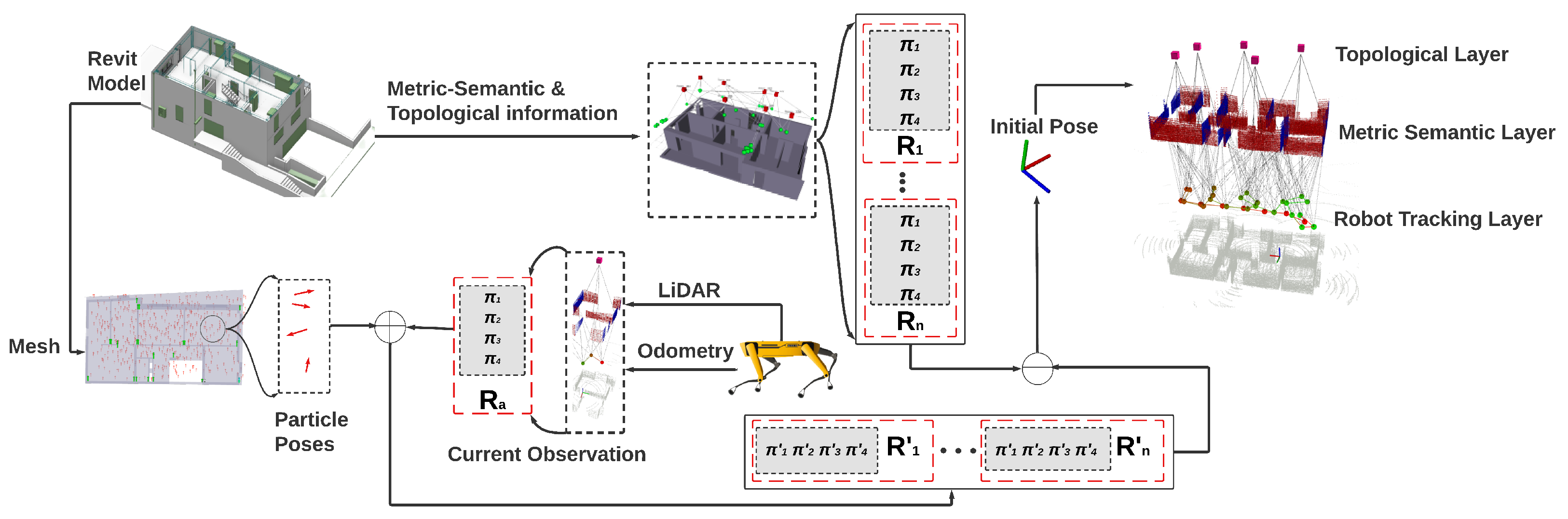
Figure 1.
Visualization of the proposed approach. Initially, the S-Graph’s topological and metric-semantic layers are generated by extracting data from a building’s architectural plan, made in Revit. Each room R’s four walls are denoted by , , , and . Following that, a particle filter is initialized, and particles are dispersed throughout the entire environment. As the robot navigates the environment, it observes the walls and rooms. These observations are converted into each particle’s frame of reference, and global localization is achieved by comparing them to the data extracted from the architectural plans. Finally, the robot tracking layer is added to the S-Graph created in the first step.
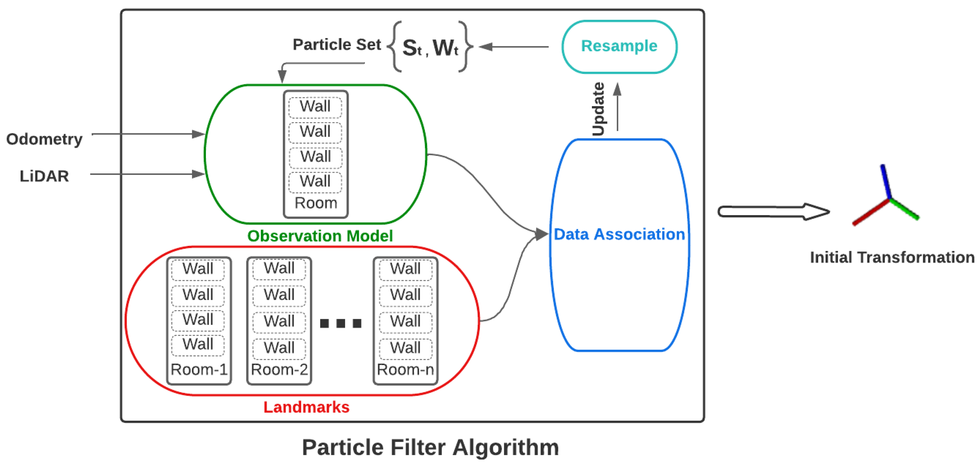
Figure 2.
Particle filter algorithm overview. Walls and rooms are detected by using robot odometry and LiDAR data and transformed into each particle’s frame. These observations are then associated with landmark walls and rooms extracted from the architectural plan. Afterward, the particle weights are updated and resampling is performed which eventually gives the initial transformation upon convergence.
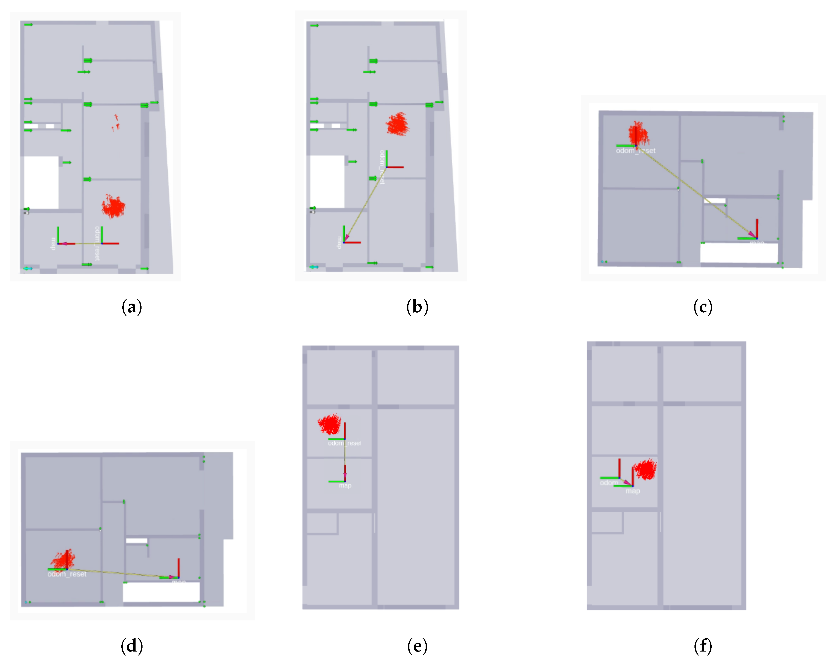
Figure 3.
Top view of the particle filter localization with topological rooms information (a) The particles are initialized in the entire floor. (b) Particles form two clusters after the update step. Note the ’clusters’ are formed in 2 rooms with similar geometry. (c) The particles successfully converge in the correct room and the initial pose is published.
Figure 4.
Top view of the initial transformation estimation by our approach in various environments. (a) sequence; (b) sequence; (c) sequence; (d) sequence; (e) sequence; (f) sequence.
Figure 4.
Top view of the initial transformation estimation by our approach in various environments. (a) sequence; (b) sequence; (c) sequence; (d) sequence; (e) sequence; (f) sequence.
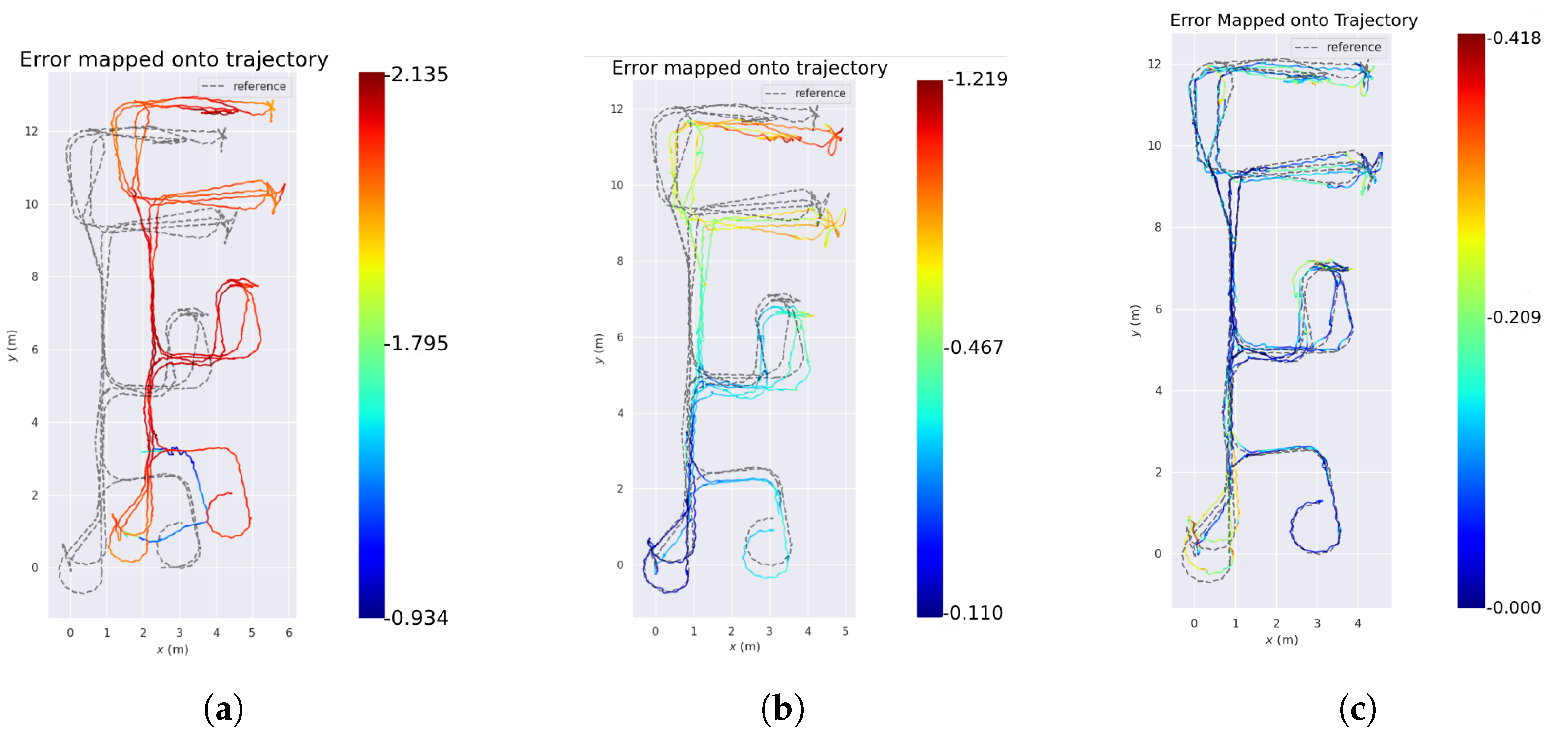
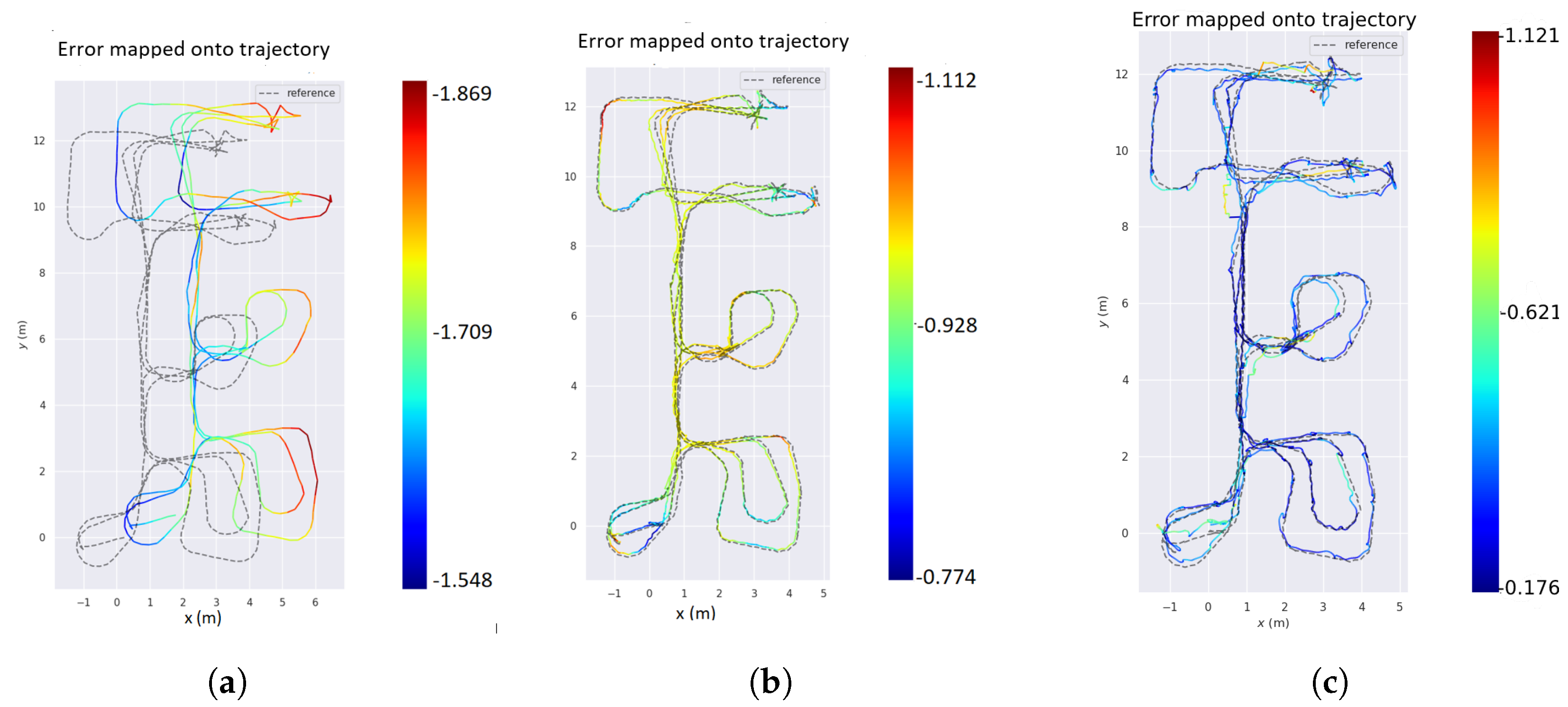
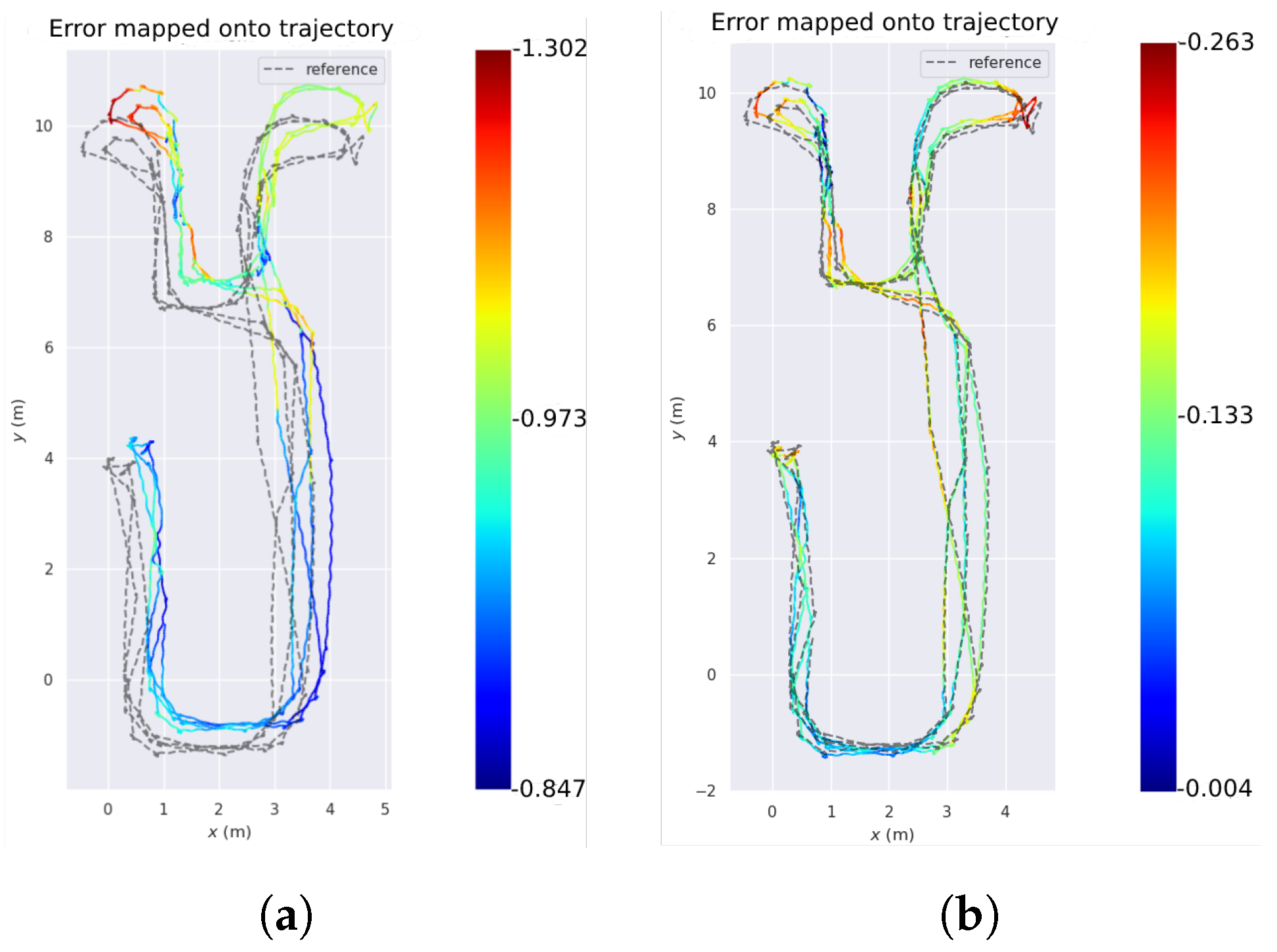
Figure 5.
Top view of estimated trajectories for all baselines and our S-Graph Localization in the sequence of our simulated data. The dotted line shows the ground truth trajectory. Our S-Graph Localization presents the lowest errors followed by UKF localization. (a) AMCL ; (b) UKFL ; (c) S-Graph Localization .
Figure 6.
Top view of estimated trajectories for all baselines and our S-Graph Localization in the sequence of our simulated data. The dotted line shows the ground truth trajectory. Our S-Graph Localization presents the lowest errors, followed by UKF localization. (a) AMCL ; (b) UKFL ; (c) S-Graph Localization .
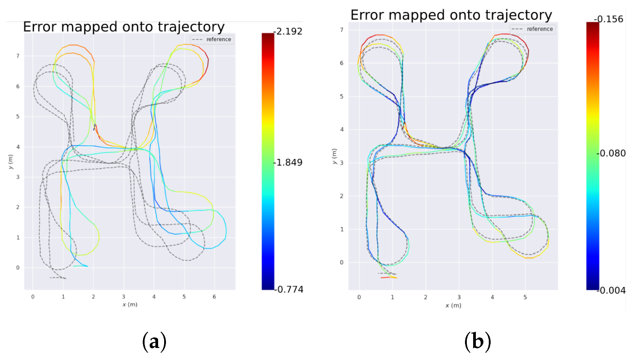
Figure 7.
Top view of estimated trajectories for our S-Graph Localization and AMCL in the sequence of our simulated data. The dotted line shows the ground truth trajectory. UKF localization failed to localize in this dataset. (a) AMCL ; (b) S-Graph Localization .
Figure 7.
Top view of estimated trajectories for our S-Graph Localization and AMCL in the sequence of our simulated data. The dotted line shows the ground truth trajectory. UKF localization failed to localize in this dataset. (a) AMCL ; (b) S-Graph Localization .
Figure 8.
Top view of estimated trajectories for all baselines and our S-Graph Localization in the sequence of our simulated data. The dotted line shows the ground truth trajectory. Our S-Graph Localization presents the lowest errors, followed by UKF localization. (a) AMCL ; (b) UKFL ; (c) S-Graph Localization .
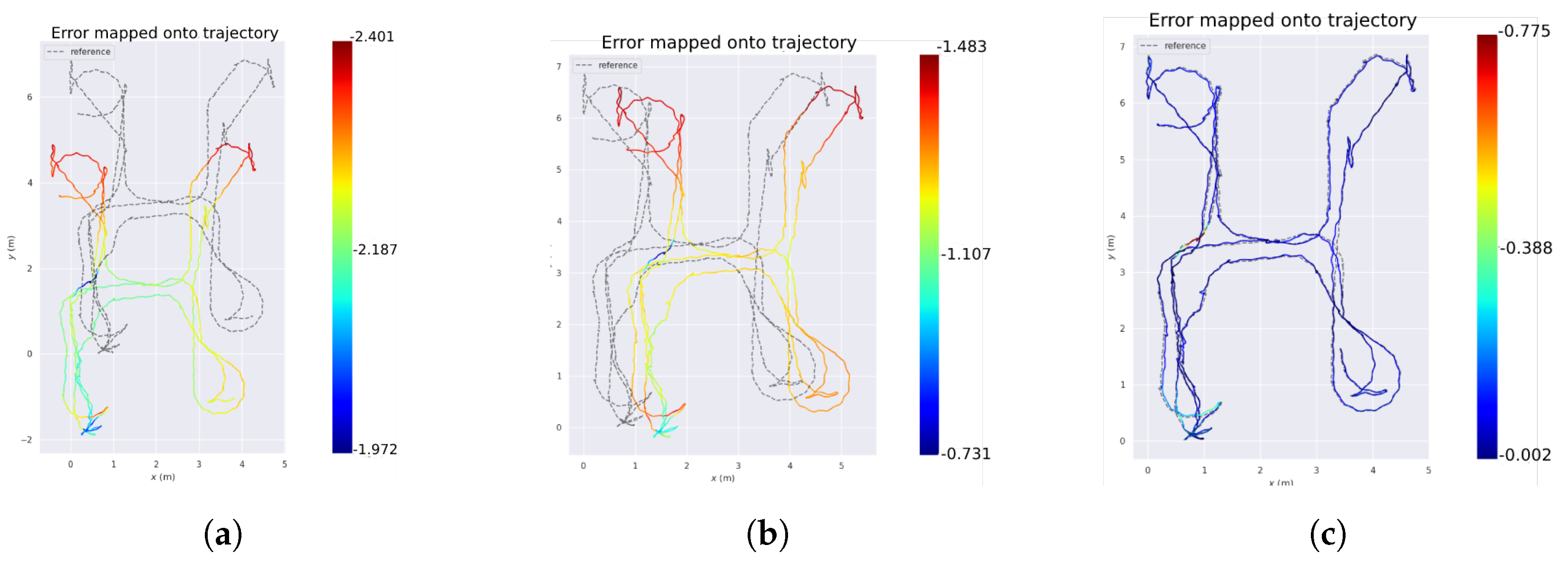
Figure 9.
Top view of estimated trajectories for Our S-Graph Localization and UKF localization in the sequence of our simulated data. The dotted line shows the ground truth trajectory. AMCL failed to localize in this dataset. (a) UKFL ; (b) S-Graph Localization .
Figure 9.
Top view of estimated trajectories for Our S-Graph Localization and UKF localization in the sequence of our simulated data. The dotted line shows the ground truth trajectory. AMCL failed to localize in this dataset. (a) UKFL ; (b) S-Graph Localization .
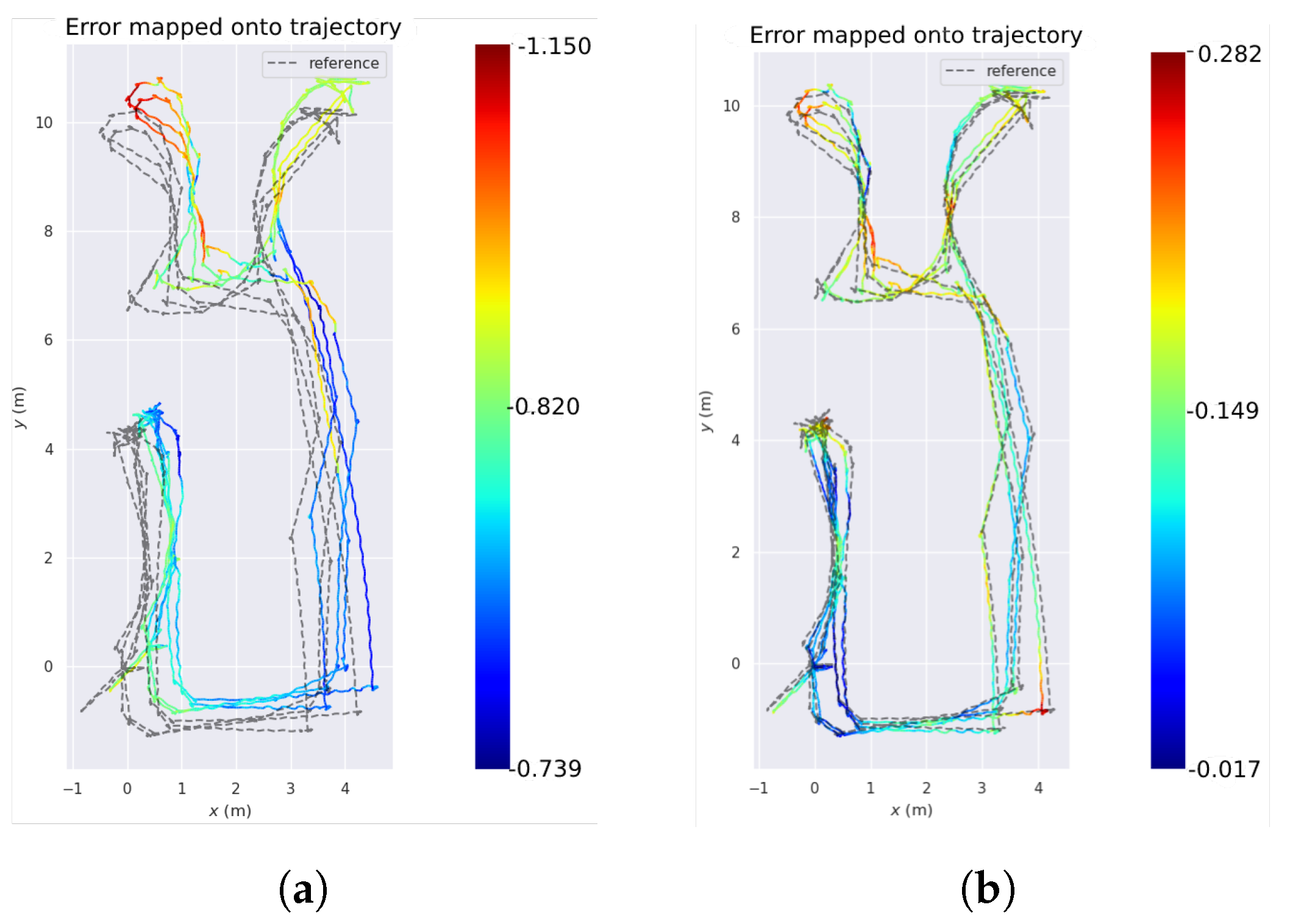
Figure 10.
Top view of estimated trajectories for Our S-Graph Localization and UKF localization in the sequence of our simulated data. The dotted line shows the ground truth trajectory. AMCL failed to localize in this dataset. (a) UKFL ; (b) S-Graph Localization .
Figure 10.
Top view of estimated trajectories for Our S-Graph Localization and UKF localization in the sequence of our simulated data. The dotted line shows the ground truth trajectory. AMCL failed to localize in this dataset. (a) UKFL ; (b) S-Graph Localization .
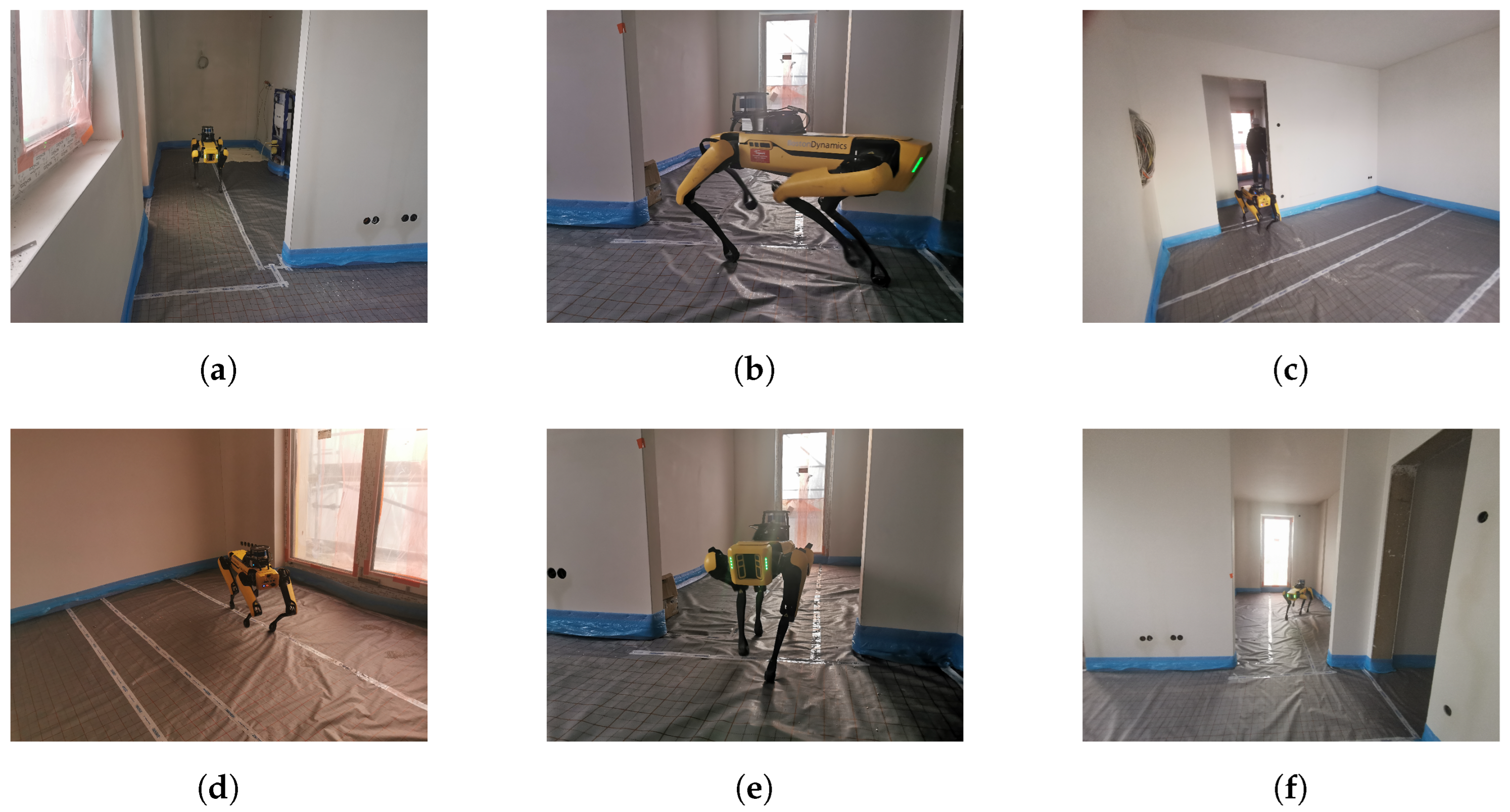
Figure 11.
Snapshots of testing of our algorithm in the real-world construction site with a legged robot. (
a–
c) show the robot being tested in environment
BM-1 and (
d–
f) show the robot being tested in environment
BM-2 as described in
Table 4.
Figure 11.
Snapshots of testing of our algorithm in the real-world construction site with a legged robot. (
a–
c) show the robot being tested in environment
BM-1 and (
d–
f) show the robot being tested in environment
BM-2 as described in
Table 4.
Table 1.
Absolute Pose Error (APE) [m] for several LiDAR-based localization baselines and our S-Graph Localization. Datasets have been recorded in simulated environments. ‘−’ stands for localization failure.
Table 1.
Absolute Pose Error (APE) [m] for several LiDAR-based localization baselines and our S-Graph Localization. Datasets have been recorded in simulated environments. ‘−’ stands for localization failure.
| Method | APE [m] ↓ |
|---|
| | Datasets |
|---|
| | D1 | D2 | D3 | D4 | D5 | D6 |
| AMCL [11] | 2.04 | 1.71 | 2.03 | 2.01 | − | − |
| UKFL [15] | 0.97 | 0.78 | − | 0.74 | 0.70 | 0.88 |
| S-Graph Localization (ours) | 0.28 | 0.15 | 0.20 | 0.24 | 0.29 | 0.22 |
Table 2.
Localization success rate of our method in our simulated datasets. Every experiment was performed 10 times for each dataset. Note that has a lower success rate because of symmetry.
Table 2.
Localization success rate of our method in our simulated datasets. Every experiment was performed 10 times for each dataset. Note that has a lower success rate because of symmetry.
| Method | Convergence Rate [%] |
|---|
| | Datasets |
|---|
| | | | | | | |
| AMCL [11] | 100 | 100 | 50 | 40 | − | − |
| UKFL [15] | 100 | 100 | − | 70 | 40 | 70 |
| S-Graph Localization (ours) | 100 | 100 | 60 | 50 | 50 | 80 |
Table 3.
Convergence Time [s] for several LiDAR-based localization baselines and our S-Graph Localization in simulated environments. ‘−’ stands for localization failure.
Table 3.
Convergence Time [s] for several LiDAR-based localization baselines and our S-Graph Localization in simulated environments. ‘−’ stands for localization failure.
| Method | Time [s] ↓ |
|---|
| | Datasets |
|---|
| | | | | | | |
| AMCL [11] | 22 | 27 | 76 | 69 | − | − |
| UKFL [15] | 16 | 25 | − | 83 | 88 | 71 |
| S-Graph Localization (ours) | 16 | 23 | 72 | 69 | 73 | 65 |
Table 4.
Point cloud alignment error [m] on the real datasets. The best results are boldfaced, second best are underlined.
Table 4.
Point cloud alignment error [m] on the real datasets. The best results are boldfaced, second best are underlined.
| | Alignment Error [m] ↓ |
|---|
| | Datasets |
|---|
| Method | BM-1 | BM-2 | BM-3 |
|---|
| AMCL [11] | 0.98 | − | − |
| UKFL [15] | 0.43 | 0.27 | 1.03 |
| S-Graph Localization (ours) | 0.285 | 0.25 | 0.99 |
Table 5.
Convergence Time [s] for our S-Graph Localization in simulated environments without the Topological factor. The convergence time increases without the topological factor.
Table 5.
Convergence Time [s] for our S-Graph Localization in simulated environments without the Topological factor. The convergence time increases without the topological factor.
| Method | Time [s] ↓ |
|---|
| | Datasets |
|---|
| | | | | | | |
| S-Graph Localization (ours) | 27 | 33 | 97 | 93 | 115 | 103 |
Table 6.
Localization success rate of our method without topological factor in our simulated datasets. Every experiment was performed 10 times for each dataset.
Table 6.
Localization success rate of our method without topological factor in our simulated datasets. Every experiment was performed 10 times for each dataset.
| Method | Convergence Rate [%] |
|---|
| | Datasets |
|---|
| | | | | | | |
| S-Graph Localization (ours) | 50 | 50 | 30 | 30 | 20 | 40 |
Table 7.
Absolute Pose Error (APE) [m] without topological factor in our simulated datasets.
Table 7.
Absolute Pose Error (APE) [m] without topological factor in our simulated datasets.
| Method | APE [m] ↓ |
|---|
| | Datasets |
|---|
| | | | | | | |
| S-Graph Localization (ours) | 0.30 | 0.16 | 0.20 | 0.24 | 0.31 | 0.23 |


