1. Introduction
Minimally invasive surgery is being adopted over traditional surgical methods due to its ability to improve patient outcomes. In these procedures, compliant, flexible continuum devices such as catheters are inserted through a single small incision. The flexible nature of catheters reduces stress on surrounding tissue. Autonomous control of these devices has advantages over traditional surgery because it can achieve extreme accuracy and stability even beyond that of a trained surgeon [
1]. Robotic minimally invasive methods also increase dexterity when compared to manually guided devices, as flexible catheters can be navigated through cavities to specific targets within the body [
2]. Magnetic control of continuum surgical devices is an effective solution for a broad range of surgical applications, including cardiac ablation [
3], inserting cochlear implants [
4], and optometry [
5].
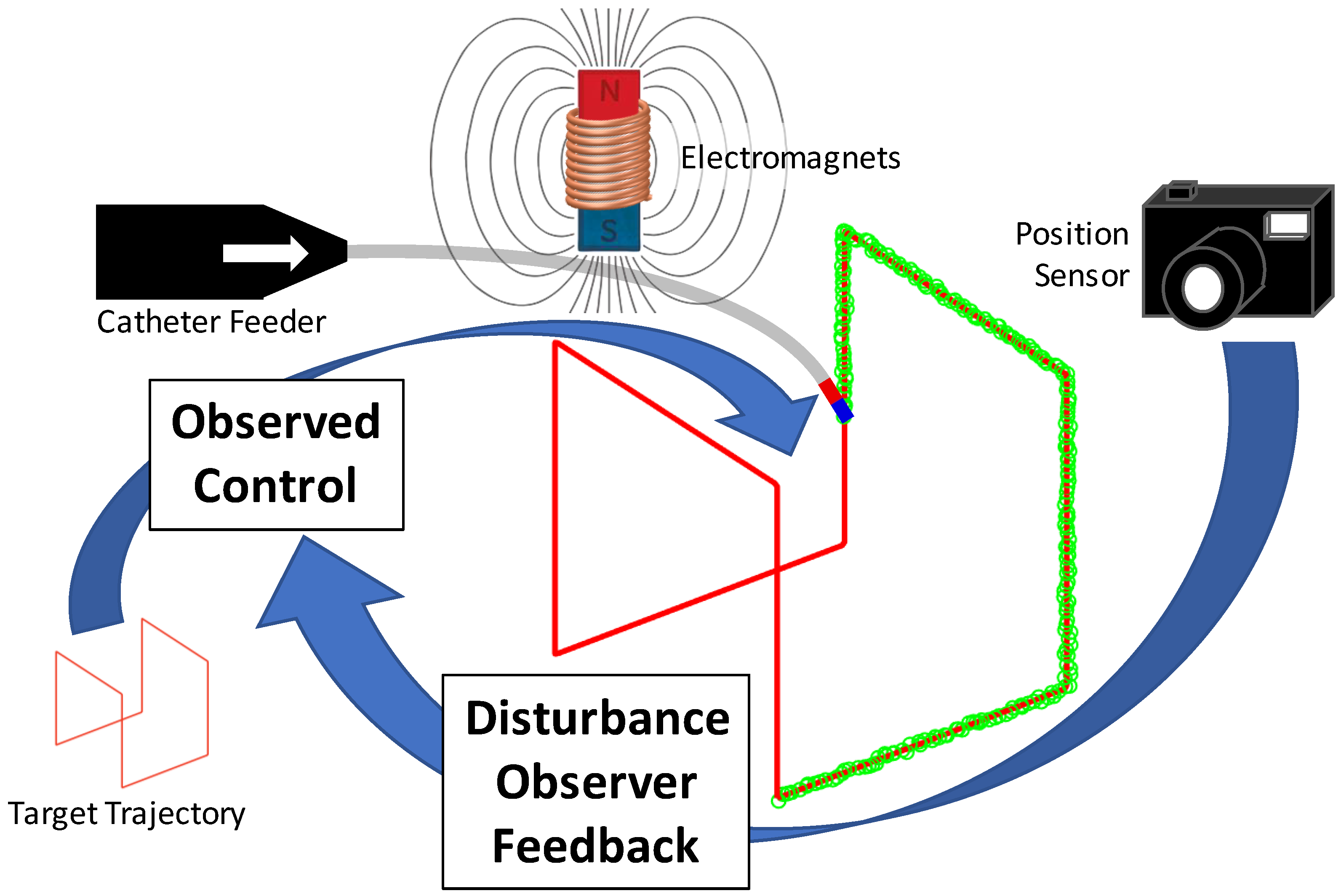
Here we propose steering a flexible magnetic catheter using a new approach named
observed control, which employs the well-established Kalman smoother framework to perform model-based predictive control. As shown in the
Figure 1 system diagram, we use observed control to predict open-loop inputs to position the catheter tip on the desired trajectory. A disturbance observer uses positional feedback to calculate model disturbances that explain trajectory error. Finally, controls are applied to correct for these disturbances, resulting in closed-loop control of an extensible magnetic catheter.
Other methods currently exist to control magnetic catheters in real-time. Sikorski et al. modeled the catheter as a pseudorigid-body and used stereo vision to get shape feedback from a 3D point cloud [
2]. This method achieved sub-millimeter trajectory tracking accuracy. However, this control method is currently only possible when the entire catheter is in view of a camera. Hybrid position and force control has also been used to localize catheters in vivo. Heunis et al. visualized a catheter in the vasculature using a multi-modal approach, including ultrasound imaging and Fiber Bragg sensors [
8]. Kratchman et al. suggested that open-loop control might be sufficient for magnetic steering after calibrating a system with visual feedback [
9]. However, the flexible nature of soft tissue could cause the desired trajectory to shift during surgical procedures, so measurements and feedback may be necessary for control. Boskma et al. achieved accurate magnetically steered closed-loop control through ultrasound imaging [
10].
Magnetic catheter devices have been implemented using various methods. Previously, micro coils have been embedded into surgical instruments and controlled by inducing a current using an MRI machine [
11]. Variable stiffness catheters can be used to augment magnetic steering [
12]. Permanent magnets embedded into catheter tips can be used in conjunction with variable strength external electromagnets [
9,
13,
14,
15]. In 2006, Tunay et al. used elliptic integrals to model the magnetic field and used a closed-form solution of magnetic torque and reaction forces to estimate the shape of a catheter using Euler-Bernoulli beam theory [
16]. However, this method uses small angle assumptions that break down in complex catheter geometries [
17]. Model-less methods have been explored for cardiac ablation procedures using position and force control [
18]. Cosserat rod theory has been used to model catheters in conjunction with the implicit collocation method to find the state of a magnetic catheter when subject to an external magnetic field [
19]. In their work, Edelmann et al. developed a general catheter model capable of multiple alternating flexible and magnet segments and demonstrated control experimentally on a system of one permanent magnet embedded in the tip of the catheter and steered with external electromagnets [
19]. However, control Jacobians needed to be developed separately from the Cosserat solver to recover the effect of magnetic and insertion control on catheter shape [
19]. Complexity in modeling has resulted in a lack of model-based planning control for magnetic catheters, which may offer a refinement over existing Jacobian-based control methods.
1.1. Planning Methods
While most system models predict a new state based on current states and controls, planners solve the model inverse problem: finding control inputs that achieve a desired state. Planning is inherently an optimization problem that requires a predictive model and minimizes an objective function. Implementations of these functions are diverse and include various conditions, but in their most simple form, they optimize for controls that minimize the state error from a desired target. No motion planning methods have previously been presented for magnetic catheters.
Model-based planning is a well-studied field, with frameworks available for outlining and visualizing planning problems, which are solved and implemented in a variety of problem-specific approaches. Among these general frameworks are model predictive control (MPC) and factor graphs. MPC is a control framework that includes a predictive step that is effectively motion planning, followed by a sensor feedback step [
20]. After the optimized controls are executed, sensor feedback is incorporated to estimate the new state, which is used as the new initial condition in the next cycle, resulting in continuous closed-loop control. Factor graphs are generalized structures that represent complicated functions as probabilistic factor nodes and variable nodes connected by edges that indicate dependency [
21]. MPC and factor graphs provide a framework and visualization for setting up a planning problem, but they do not specify cost functions or optimization methods to use in solving the problem. Nevertheless, both methods have been implemented very successfully. With MPC, nonlinear control problems are often solved using numerical Newton-type optimization schemes, such as collocation as implemented by Hedengren et al. [
22].
While probabilistic inference with factor graphs has historically been used as a foundation for state estimation, recent work has advanced its use in planning. This approach naturally pairs with Markov methods, as Attias proposed using it to solve a partially observable Markov decision process (POMDP) [
23]. With the help of factor graphs to identify sparsity, Mukadam et al. developed an efficient motion planning method using Gaussian process factors formed as a Gauss–Markov chain [
24]. In their work, Mukadam et al. also present the use of fictitious observations with low uncertainties to be used as constraints. In particular, they implement fictitious measurements of a target state with low covariance as a constraint in their planning optimization, which results in optimal controls to achieve that target state.
While not always explicit, state estimation is integral to planning and control. However, state estimation and planning have historically been treated as separate problems. By leveraging their overlap, significant efficiency improvements over independent approaches can be achieved. In 2014, Penny introduced a simultaneous localization and planning (SLAP) framework to simultaneously compute the current state estimate and a new plan using probabilistic inference with a hidden Markov model (HMM) [
25]. Ta et al. also implemented simultaneous estimation and control using factor graph-informed inference and MPC [
26]. In 2019, Mukadam et al. generalized SLAP into their simultaneous trajectory estimation and planning (STEAP) method, which computes the full continuous-time trajectory conditioned on observations and costs in both the past and the future using Gaussian processes [
27]. In our work, we apply this approach to flexible continuum devices by leveraging a Kalman smoother framework for computation.
1.2. Control Methods
Control does not require planning and can be purely error based, such as proportional-integral-derivative (PID) control. While often effective, this simple control suffers robustness limitations in nonlinear systems. Planning can often be used to create a control strategy that leads to more robust real-time nonlinear control. However, model-based control has not yet been explicitly implemented for magnetic catheters.
All previous approaches to steer Cosserat rod catheters use Jacobian inverse control. Computing a control Jacobian for such a complex model is difficult, so many previous methods have chosen simplified models such as Euler–Bernoulli to obtain a control Jacobian. In 2017, Edelmann et al. explicitly computed the control Jacobian for the full magnetically controlled Cosserat rod catheter model [
19]. They used this linearized control sensitivity with proportional-derivative (PD) control to guide the catheter with closed-loop positional feedback [
19]. However, not only is this Jacobian complex to derive, it is difficult to implement. It requires computing Jacobians iteratively for each segment and then integrating these Jacobians in reverse order back down the length of the catheter. Additionally, while effective for a single magnet catheter, this control method does not scale well with multiple catheters, as a new control Jacobian would need to be derived. Here we instead propose a more accessible control approach. Observed control provides an adoptable way to find controls in a complex model without explicitly deriving a control Jacobian, as the calculations are implicitly handled in the smoothing algorithm. Due to its generalized structure, our method is also applicable to any catheter model, including a system of multiple devices.
Thus, the primary contribution of this work is introducing observed control, which is a generalizable model-based controller and demonstrating its advantages in closed-loop control of a magnetic robotic catheter. Observed control predicts controls that achieve a desired state using the Kalman smoother framework by including desired target conditions as measurements to estimate the controls needed to navigate the catheter to a desired position. We use this same Kalman smoother framework to solve a Cosserat rod model concurrently for shape and controls. Finally, sensor measurement data is incorporated using this framework as a state observer to provide model-based closed-loop feedback control and increase catheter position accuracy. In summary, we solve for catheter shape, predictive controls, and closed-loop control from observer feedback, all within this same Kalman smoother framework.
2. Observed Control
Observed control is a model-based controller that optimizes a state space model for control inputs to achieve a desired condition from the current state. Observed control lies at the intersection of MPC and factor graph motion planning. As in MPC, observed control requires a predictive model, an algorithm to optimize for controls, and a cost constraint. Additionally, both incorporate sensor feedback for closed-loop control. As with factor graphs, observed control implements a Bayesian-inspired representation for planning, estimation, and constraints.
A primary advantage of observed control over MPC and factor graphs is implementing a Kalman smoother as a convenient optimization method and constraint framework. Both MPC and factor graphs often require problem-specific implementations because they just outline solving approaches without specifying exact methods. To provide a general functional methodology, observed control leverages the heritage of the Kalman smoother framework’s well-defined and efficient optimization approach, while Kalman measurement updates provide a standardized method to implement cost constraints. The most simple implementation of observed control then only requires a dynamic model and a desired condition, such as a target state, to solve for control inputs.
2.1. Smoother Framework
Since the states are not directly known but are observable, observed control can be formulated as a POMDP if the Markov property is held. In accordance with this property, observed control state space models follow the generic discrete nonlinear form in (1), which is adapted from the Gauss–Markov model generated from a stochastic differential equation [
28].
with
and
, and where
is the unknown process noise covariance,
are the unknown independent measurement noise covariances,
are the corresponding measurement models, and
is the state transition function from time
n to
. Subscript
indicates different measurement models and associated measurements. Subscript
indicates that measurements are time independent from model updates indicated with subscript
.
Adhering to the Markov property is a prerequisite of Kalman smoothing. A Kalman smoother minimizes the variance of the output estimation error of a given dataset for a linear system model. Structuring observed control models in the form of Equation (1) allows for inference with a nonlinear Kalman smoother [
28]. While many nonlinear Kalman smoother implementations are available, we chose the extended Kalman smoother (EKS) for this application since it is a well-established method to estimate state and state covariance using model dynamics and measurements in nonlinear applications [
29,
30,
31,
32,
33]. EKS applies linear Kalman smoothing to first-order local linearizations of a nonlinear system. The generic system in Equation (1) can be linearized using a first-order Taylor series expansion so that it can be approximated as the following time-varying linear system and smoothed using the EKS:
A full explanation is omitted for brevity, but the Extended Kalman filter (EKF) forward pass equations of the EKS are summarized in Equations (3) and (4).
Predict State:
where
and
are the
a priori state estimate and covariance, and
k includes all previous measurement
and model
n updates.
Measurement Update:
where
is the measurement residual,
is the innovation covariance,
is the Kalman gain, and
and
are the
a posteriori state estimate and covariance.
We employ the Rauch, Tung–Striebel (RTS) smoother type of the EKS as given in [
34]. A full explanation is again omitted, but the backward pass “smoothed” variables are summarized in Equation (5). Numerical integration of the state and sensitivity matrices in the EKS is computed using the Dormand–Prince 8th order Runge–Kutta integrator [
35].
The iterated extended Kalman smoother (IEKS) repeats the EKS until it converges since, due to the nature of nonlinear systems, it is not guaranteed to be optimal in one pass [
36,
37]. Observed control uses the smoother to find certain boundary conditions, so they will necessarily have inaccurate initial values. Multiple smoothing passes with IEKS converge these values to the desired accuracy.
2.2. Smoother Modifications
To use the smoother framework to find controls, the controls must be treated as states, and their associated dynamics included in the predictive model. This allows for the smoother to converge their values concurrently with the states. The traditional smoother control vector and control updates are not used, as controls are instead augmented to the state vector:
Desired conditions are encoded as measurements as in Equation (
1b) and implemented as Kalman measurement updates as shown in Equation (4).
is set as the desired condition and its relationship to the state is encoded in
, which in the EKF is linearized at
m as
. Similarly to [
24], these fictitious measurements effectively fix the desired conditions in the smoother by setting low measurement covariances
. Disallowing uncertainty in the measurement forces the smoother to manipulate states such that the desired condition is met. If low covariances are also set on assumed conditions such as known current states, then the remaining states, namely the augmented control states, are optimized by the smoother to achieve the desired condition. This is the principal operation of observed control.
Taking the case of a desired full state target condition as an example; if
is the number of traditional states and
is the number of controls, then:
Due to their zero covariance, the desired traditional states cannot be affected in the Kalman smoother. Thus, the control states must account for transitioning from the current state to the desired state.
More generally, this framework allows for any constraint to be applied, not just desired state conditions. Constraints need only relate to the states as described by independent measurement models for each constraint type, and observed control can implement any number of that type of constraint at desired points in m as . This implies that conditions can be applied to effectively change the cost function without requiring any changes to the underlying optimization method.
Note that we choose a low covariance and not a zero covariance for assumed and desired conditions implemented as measurements. Initial state covariances can be exactly zero, but measurement covariances should not be to ensure the numerical stability of the Kalman smoother algorithm. Zero measurement covariance allows the innovation covariance matrix
to be poorly conditioned, and this matrix is inverted to calculate the Kalman gain as shown in Equation (
4c). Because singular matrices are not invertible, too small of measurement covariances make this inversion numerically unstable. Thus, we choose them to be appropriately small to minimize uncertainty in fixed conditions but not so small that the algorithm becomes unstable. We found two orders of magnitude below the desired constraint accuracy to be a good choice generally.
3. Catheter Dynamic System
The magnetic catheter system consists of a flexible catheter embedded with permanent magnets. Since the permanent magnets are far stiffer than the flexible catheters, we model the catheter system as a series of flexible (non-magnetic) and (rigid) magnetic segments as in [
19]. The catheter model is designed to include any number of flexible and magnetic segments, with each segment having its own specific material properties. Each segment is described by the Cosserat rod states: position
, quaternion
, force
, and torque
, as shown in Equation (
7). Distal properties of preceding segments are proximal properties of following segments, ensuring continuity throughout the catheter.
Cosserat rod theory is used to model the flexible segments because it has been demonstrated to be accurate in handling large deflections [
19]. This is advantageous over less robust methods such as Euler–Bernouli beam theory, which is only accurate for a limited range of bending angles [
13]. The catheter is assumed to be in static equilibrium, and the only external forces and torques acting on the catheter are assumed to be from gravity, magnetic interactions, and distal and proximal loadings.
3.1. Shape Equations
Cosserat rod shape equations are available elsewhere in the literature (e.g., [
19]) but are reproduced here for completeness. The pose transformation of magnetic segments with respect to arc length
s is given by rigid-body kinematics:
where subscript
stands for the proximal end,
is the direction of the rod axis in its body frame, and the rotation matrix
can be calculated using Rodrigues’ rotation formula [
38]. The magnetic segment wrench transform can be calculated using a static force and torque balance:
where
L is segment length,
is the total external force applied to the segment, including gravity and magnetic force,
is the total magnetic torque, and
maps the vector cross-product into the skew-symmetric matrix form. The external force is assumed to act as a point force at the segment’s centroid.
The Cosserat rod equations for the flexible segments are expressed in differential form:
where
is the direction of the centerline tangent in the rod’s reference frame,
is the intrinsic curvature of the rod in the reference frame,
is the external force per unit length applied to the segment,
is the external torque per unit length applied to the segment, and
and
are the shear-extension and bending-torsion stiffness matrices, respectively. These 13 coupled nonlinear differential equations describe how an initial pose and wrench evolve over the length of a flexible rod segment to a final pose and wrench.
3.2. Model Control Inputs
Catheter controls include an electric current vector
and a proximal segment length
L for insertion control.
contains a scalar current corresponding to each electromagnet in the field emitter, which combines to induce a magnetic field. Rigid magnetic segments respond to the applied magnetic field via a wrenching force and torque in accordance with [
39]:
where
is the intrinsic dipole moment of the embedded magnet,
describes how the field at a point varies with the control currents,
describes how a vector packing of the field-gradient varies with the control currents, and
is a matrix packing of the permanent magnet’s dipole moment [
19].
Both
and
vary across the workspace and can be obtained from a calibrated model of the magnetic system. Our system is calibrated per [
40] as a uniform field model since the emitter is set up in a Helmholtz configuration. This restricts our magnetic manipulation of the catheter to only torque control and not gradient, but there is no disadvantage, as there are still sufficient degrees of freedom for full control of the tip position of a single-magnet catheter.
To incorporate this magnetic wrench in the Cosserat rod model, we include it in
and
in Equation (
9):
Flexible segments are not affected by the magnetic wrench, but
still applies to
in Equation (
10) to account for the weight of the rod.
For catheter insertion control, our implementation drives the catheter in the system via a feeder, which occurs at the proximal end of the first segment. This is realized in the model as a linear scaling of that segment length
L using a change in the variable. Let arc length
, where
. Substituting for
s in the Cosserat equations (Equation (
10)) is shown in Equation (
13) using the general form and integrating
s over
L to find the distal states:
Always integrating
from 0 to 1 ensures capturing the full segment regardless of its current length. The
term linearly scales the differential equations so that the rod behavior progresses appropriately given its current length. Initiating
with a value of one describes the current segment length as a proportion of its initial length:
. This segment length parameter
L can be estimated, which is necessary for observed control. Additionally, this implementation allows any flexible segment to be extensible in the model, which can apply to more complex catheter designs such as concentric tube robots.
3.3. Catheter Observed Control
When used with observed control, the catheter controls are augmented to the states, resulting in the state vector in Equation (
14).
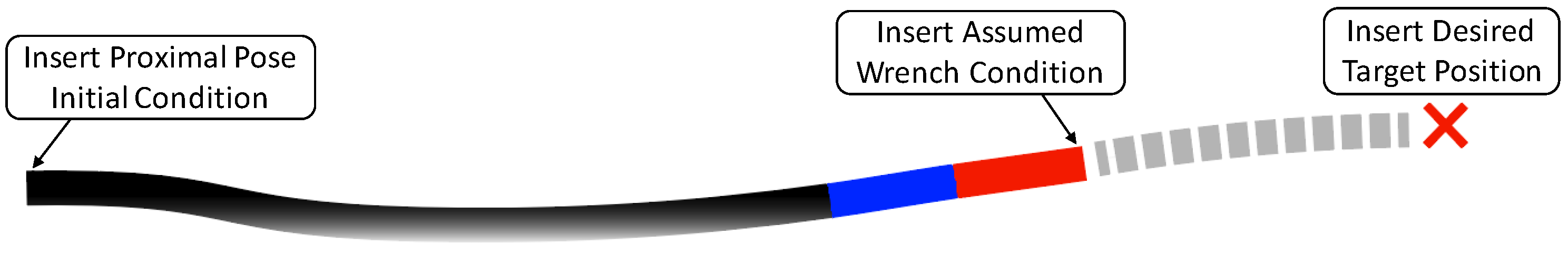
The catheter used in this application includes two segments: a proximal flexible segment followed by a distal magnetic segment. It is diagrammed in
Figure 2 in the observed control configuration. In our system, proximal pose and distal wrench boundary conditions are known. The proximal pose is an initial condition where the catheter exits the feeder. The distal wrench is assumed zero, as the rod is operating in free space. Distal wrench will be inserted as an assumed condition with low covariance. Inserted at the distal end of the catheter is a fictitious desired position condition with low covariance to convey its certainty. Using this setup, controls can be found for the catheter to achieve the desired distal position using observed control.
From a robotics dynamic system perspective, a unique aspect of the catheter equations is that they are functions of arc length along the length of the catheter, not functions of time. So when applied to this system, the smoother is also used spatially instead of temporally, as is traditional. Thus, these measurement insertions occur at distance locations along the arc length, not at instances in time. Nevertheless, the smoother and observed control framework are robust to this change in a variable, so this conceptual paradigm shift does not actually require any implementation changes.
3.4. Solving the Cosserat BVP
It is possible to calculate rod shape with forward or backward integration if all boundary conditions at a given end are known. However, because the known conditions are split between distal and proximal ends, a BVP solver is needed. Previous approaches have used implicit solvers such as collocation [
19]. We propose implementing a Kalman smoother as an explicit shooting method to find rod shape given both information of these boundary conditions and control inputs.
Hitherto, the smoother optimization framework has been explained from the perspective of observed control for finding controls given the current and desired states. However, this framework can also be used for the inverse problem: finding distal states given current states and controls. This is done by changing the conditions of the BVP and using the covariances to identify which values are fixed and which are variable. By changing the initial state covariance to zero on the augmented controls and removing the measurements of desired conditions, the smoother will perform the same optimization approach, but now the uncertainty will be resolved by manipulating the distal state to its best estimate given the initial conditions.
Table 1 visually outlined the specific conditions of states and controls for both this shape solver method and observed control.
By implementing this states-from-controls setup of the smoother framework, the Cosserat rod model can be solved for shape-given control inputs without building a complex control Jacobian and relying on its linear approximation. This can all be accomplished using the same Kalman smoother that performs observed control, thus, achieving state estimation and control within a single unified framework. Note that this shape solver approach is presented solely for comparison against previous solving methods. It is not explicitly used for planning control optimization because observed control is specifically formulated for the task.
This concept of using low covariance to indicate boundary conditions is generalizable to any conditions. It then follows that this approach can be used to solve for any combination of states and controls given sufficient known terms. Simply set low covariance for known values so they stay fixed (be it a fictitious measurement or initial condition), and the remaining output variables will converge to their optimal values given the other conditions. This allows the system to solve for any subset of states and controls all within the same smoother framework. This versatility is exploited by our closed-loop controller to observe model disturbances using sensor feedback, as described in
Section 4. The state and control conditions for this disturbance observer are shown in the last row of
Table 1.
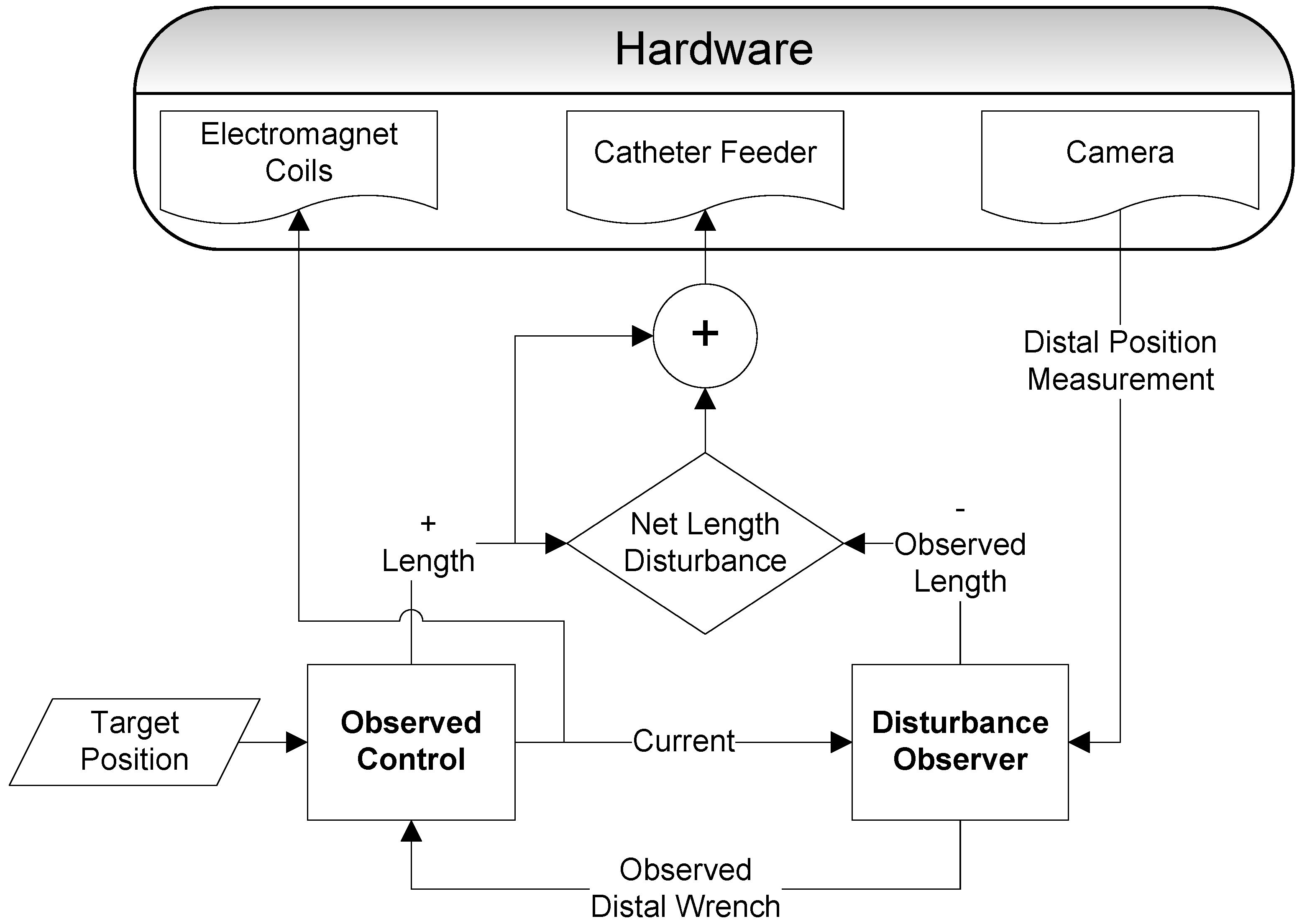
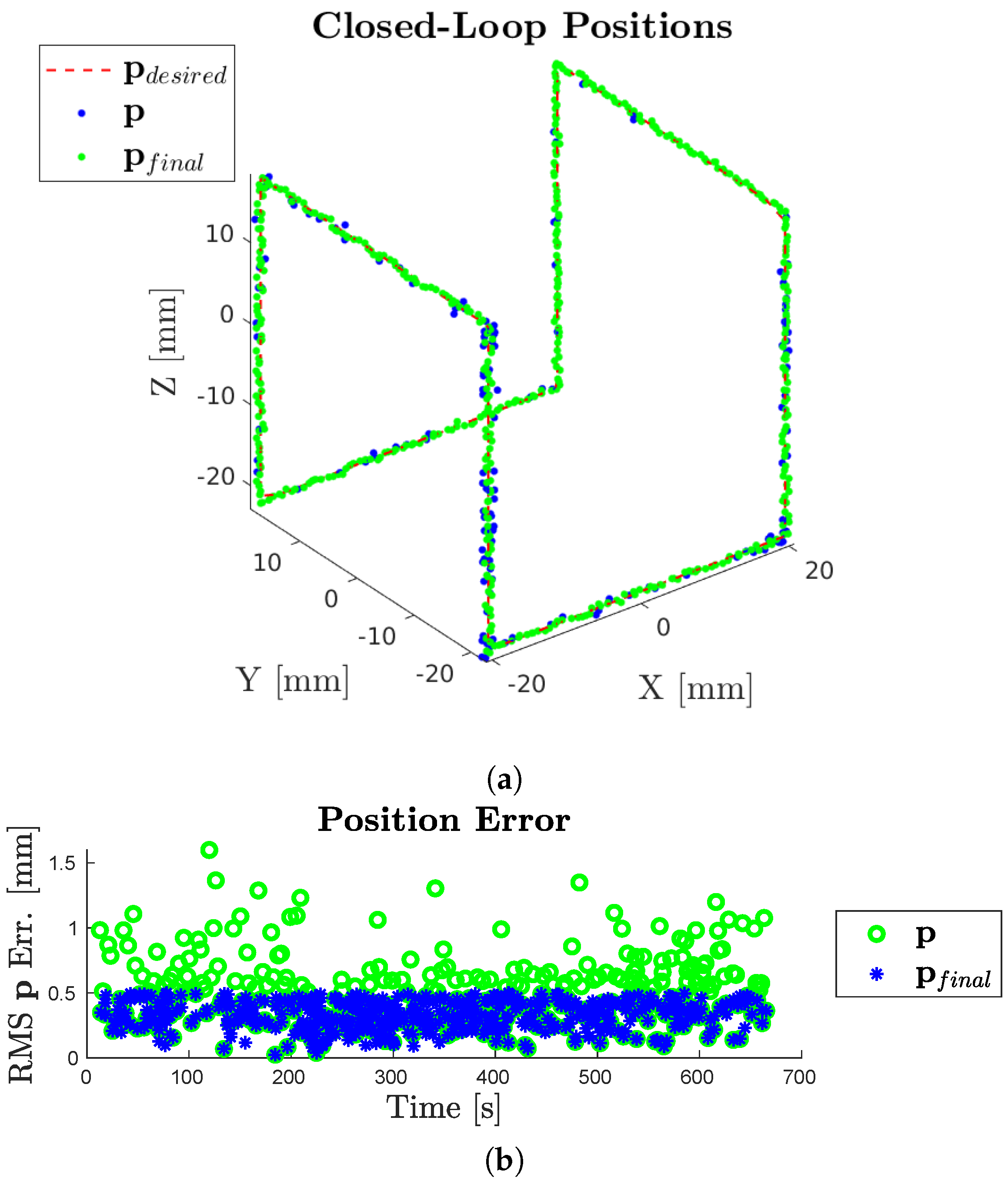
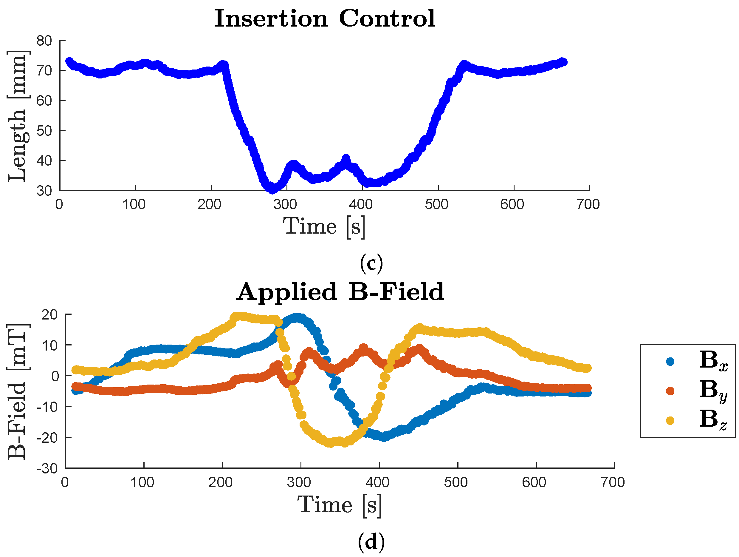
4. Closed-Loop Control
In the open loop, the observed control solves for the control current and proximal length to achieve a target distal position given a perfect model. To close the control loop, distal tip position information is used for feedback. However, because the catheter model is solved in the spatial dimension, the traditional forward-time progression feedback approach of using the sensed position as the new initial condition for the next control cycle is not applicable. Instead, we apply an observed disturbance approach. For closed-loop distal position control, a separate observer uses the distal position measurement to calculate distal wrench and length disturbances that explain positional error from the target. This process is shown in
Figure 3.
First, the observed control calculates the open-loop current and proximal segment length to achieve a target distal position, and these controls are applied to the system. Then, visual feedback provides a distal position measurement from the system. This is passed to the observer as a desired position condition. The observer takes advantage of the versatility of the smoother framework to also set the applied current control as a boundary condition and then find an effective distal wrench and proximal length to explain the sensed position deviation from the model’s expectation. The observed wrench is passed back into the observed control algorithm. Whereas initially, the distal wrench is set to zero because the catheter is in free space, now a fictitious wrench disturbance is used to explain position error. We replace the zero wrench with the wrench disturbance as a boundary condition in the observed control and continue the control loop.
Insertion control is not well encapsulated in a pure wrench disturbance due to its second-order relationship, so we handle it as a separate length disturbance. While this disturbance will handle all causes of model length inaccuracy, one illustrative example is that it can estimate slip in the feeder system. To calculate length disturbance, the observed length is subtracted from the observed control length, as shown in Equation (15). This disturbance is included in a net length disturbance, which prevents length control from oscillating between open-loop length and observed length. This net length disturbance is then added to the observed control length and applied as the control input to the system.
Because we only measure distal tip position and not full pose, we only have three degrees of freedom constrained. To maintain sufficient constraints for the BVP, we must also constrain three degrees of freedom of the distal wrench. This can be done by setting either distal force or distal torque to zero and solving for the other. In our presented experiments, we arbitrarily chose to solve for torque, as in testing, we observed both give an equivalent performance. The full distal pose could be measured to find a full distal wrench, but we found that just position measurement was sufficient for effective control.
5. Experimental Setup
5.1. Trajectory Execution
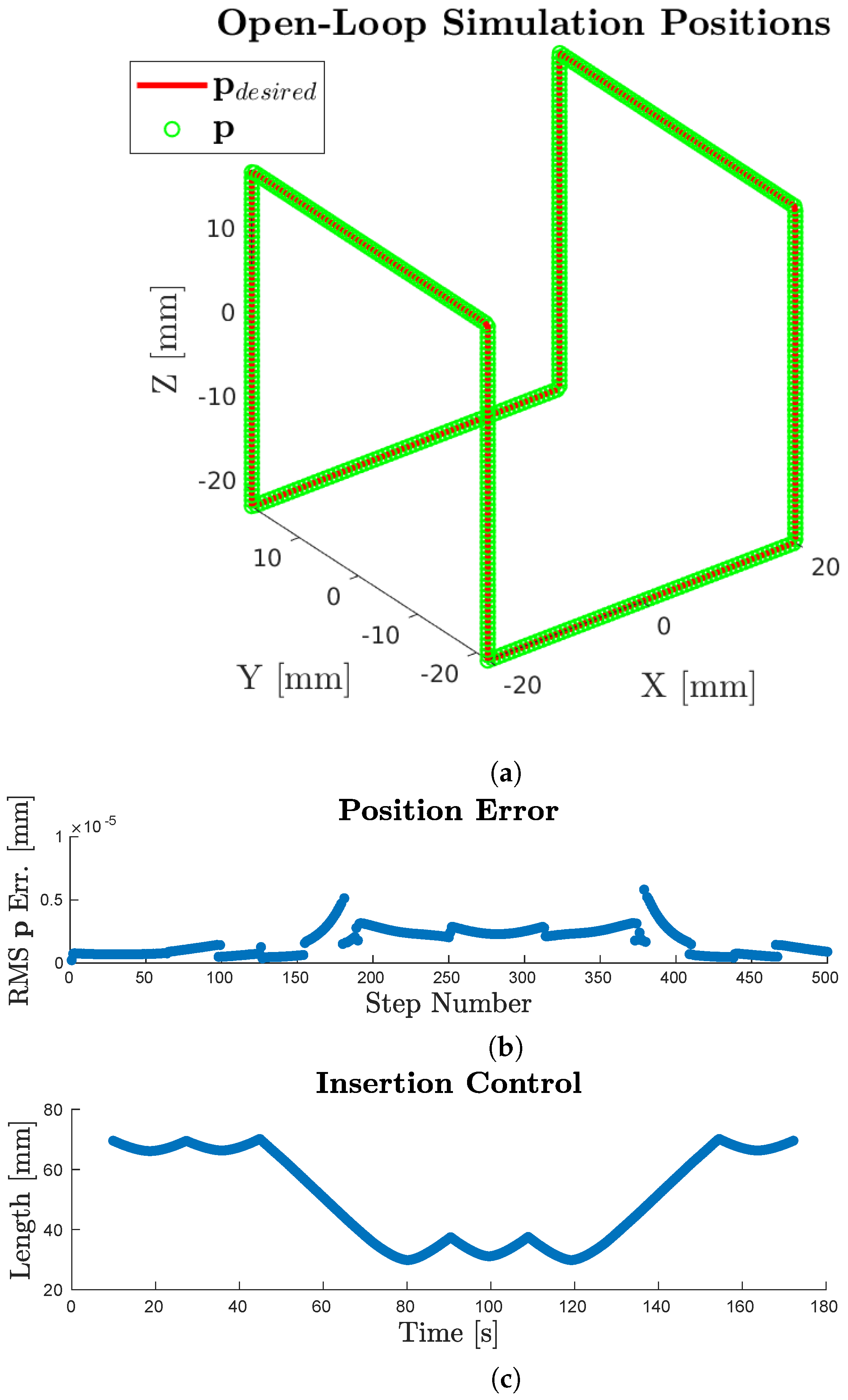
The trajectory used in this paper outlines the edges of a cube, which provides a recognizable trajectory that executes in all three spatial dimensions. The cube is scaled to 40 mm side lengths to maximize the use of the cameras’ field of view in the workspace. The proximal end at the feeder is located at the center and at the boundary of the workspace with the catheter inserted in the direction. The resolution of the target is 500 points for the full trajectory.
The trajectory is executed quasi-statically, meaning each point is treated as an independent target, and dynamics at each point, as well as between points, are ignored as the catheter moves from one equilibrium state to another. This results in the shape of the trajectory having no effect on tip position control. This is useful when the final tip position is critical, such as for an ablation procedure. This approach can also approximate a continuous trajectory target given sufficiently close sequential target points, as this will reduce convergence time and motion for each target. Thus, to execute a position trajectory, once the catheter reaches a target, the process repeats for the next target along the trajectory. Before each new solve step, the initial state covariance is reset. Additionally, for better initial conditions and continuity of the dynamic trajectory, both the wrench and length disturbances are carried over between target points.
To ignore the settling effects of each control update, the algorithm waits for the tip position measurements to settle within 0.5 mm before executing the next control. The quasi-static approach also allows for error tolerance control of final trajectory positions. The feedback control loop iterates at each target until converging below the desired 0.5 mm error tolerance.
5.2. Solve Mode Covariances
As explained in
Section 3.4, the BVP can be solved to find any condition given sufficient known conditions. In this catheter application, we use the observed control mode to find controls and the disturbance observer to find the distal wrench and proximal length. The specifics of each state’s condition for each mode were previously outlined in
Table 1. Similarly, the covariances used in practice for each condition in each mode are shown in
Table 2.
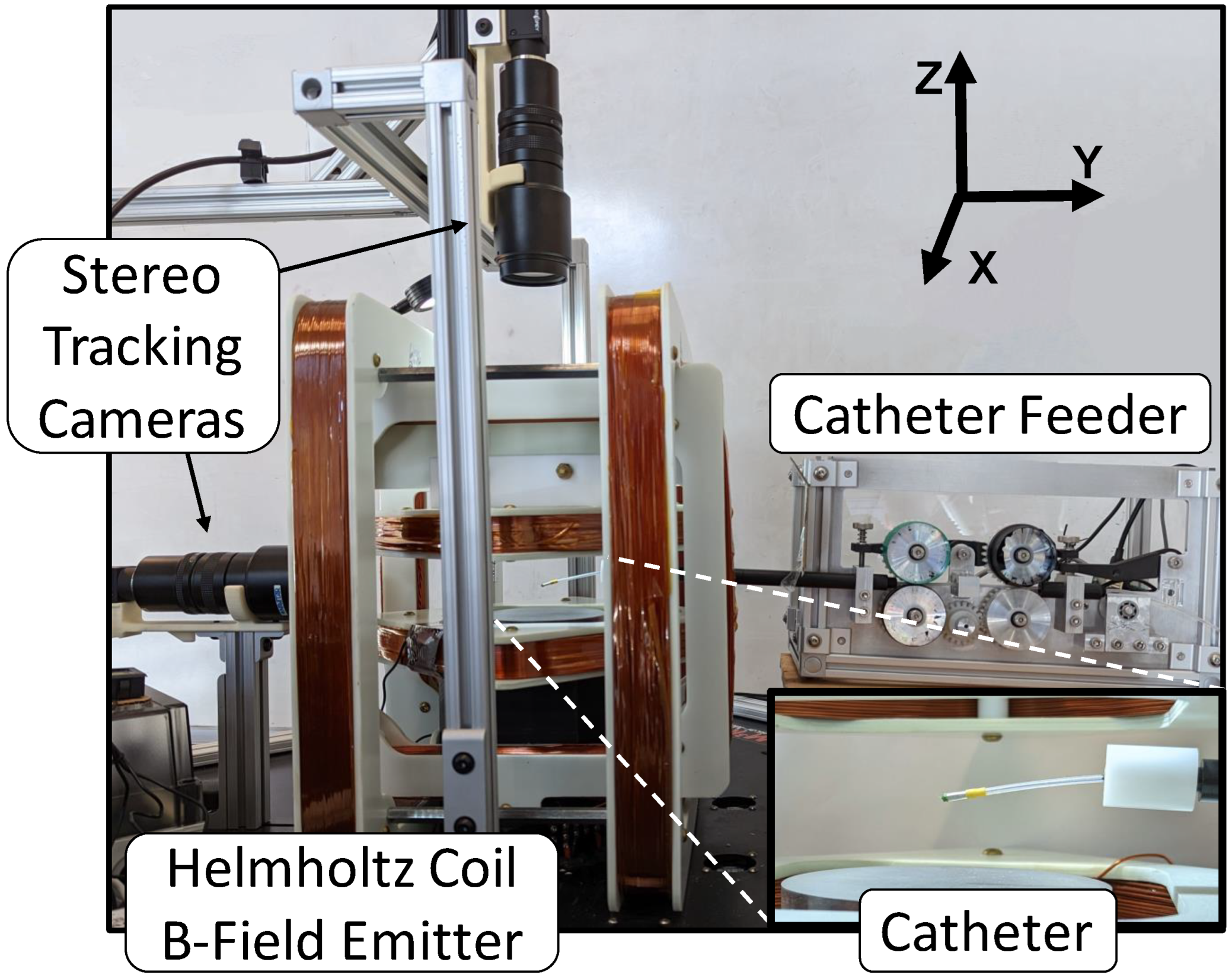
5.3. Hardware System
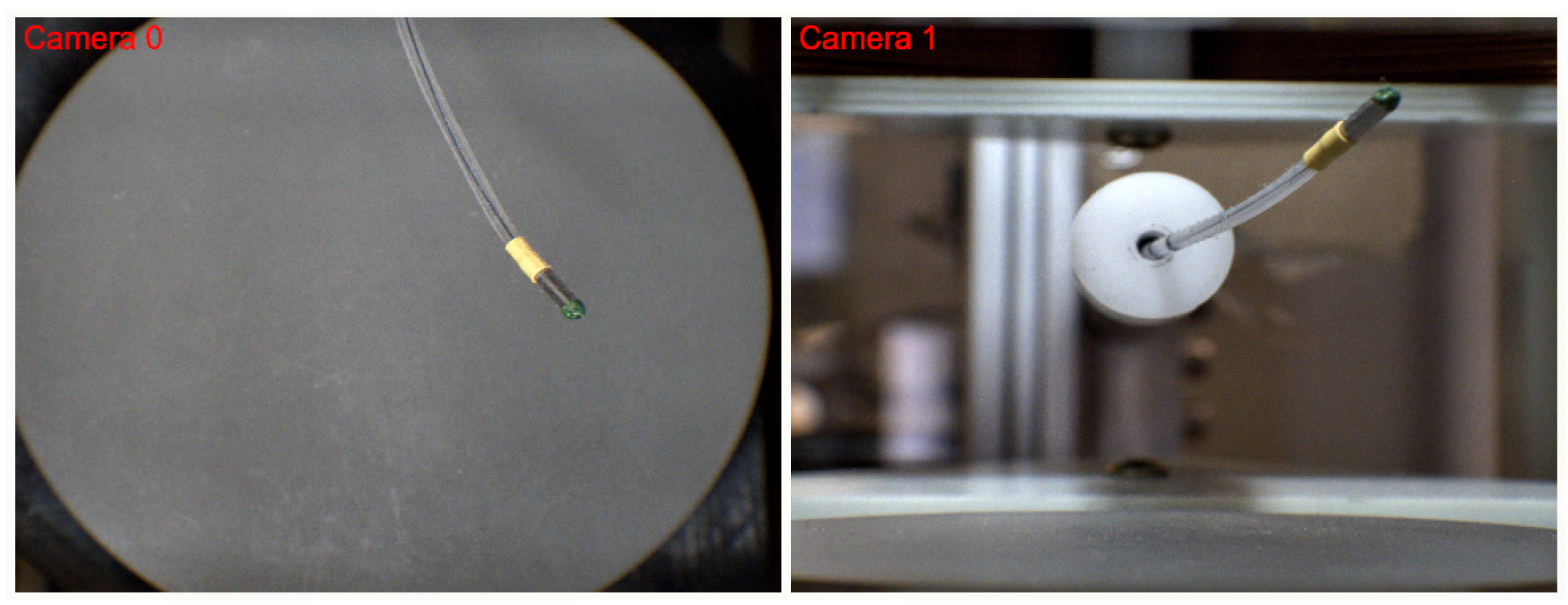
The catheter manipulation system used in this paper includes a nested Helmholtz coil system that generates a homogeneous 3D magnetic field and a feeder device that moves the catheter through tensioned rollers for linear insertion and retraction, as seen in
Figure 4. The Helmholtz coil produces a field in any direction up to 43 mT in the 140 × 140 × 50 mm workspace, and the feeder inserts the catheter up to 5 mm/s. For a detailed description of this system, see [
41]. Note that the visual position feedback and catheter design differ from [
41] and are described below.
Two BFS-U3-51S5C cameras (Point Grey, Richmond, BC, Canada) provide stereo visual feedback for 3D catheter tracking at 30 Hz. The world frame distal position of the catheter is identified using color tracking from the OpenCV library [
42] on the green-painted magnetic tip. Camera calibration is performed before testing to generate the transform from image frame pixels to world frame meters. The 480 × 402 pixel images correspond to a 100 × 84 mm overhead field of view at the bottom of the workspace, resulting in a pixel resolution accuracy of about 0.2 mm.
Shown in
Figure 5, the catheter is a 1.5 mm I.D. 2.1 mm O.D. silicone rubber sheath (McMaster-Carr, Elmhurst, IL, USA). A 0.25 mm diameter nitinol wire core (McMaster-Carr, USA) inside the silicone provides additional stiffness. The catheter tip is a 1.6 mm diameter by 9.6 mm length axially-magnetized NdFeB cylindrical permanent magnet (HKCM Engineering, Eckernförde, Germany). A yellow heat-shrink coupling is molded around the nitinol-to-magnet joint to ensure a continuous transition. The magnetic tip is pained green for color-tracking localization.
5.4. Catheter Parameters
Catheter parameters are reported in
Table 3. Various methods are used to find these values, including measuring (diameter and length), calculating (flexible segment density, magnetic density), and estimating from material properties (remanence and Young’s modulus). Magnetic material density is not an accurate parameter for the magnetic segment because the magnet is not the sole source of mass at the tip of the catheter. Additional factors include the heat-shrink coupling, the silicone sheath encasing the magnet, and the green tracking paint. Thus, effective magnetic segment density is an inflated value that accounts for these contributing masses.
7. Discussion
Experimentally, open-loop observed control was less accurate than in simulation. A calculable error is the initial position offset at the proximal end. The feeder is manually positioned, and the position error between the target and actual initial conditions will be present at each point along the entire trajectory. This error can be removed by minimizing trajectory error using a least-squares offset, which reduces the average error to 3.3 mm, as shown in the third row of
Table 4. The remaining sources of experimental error include inaccuracies in model parameters, inhomogeneity in the physical catheter, as well as the accuracy of the control hardware. While parameters could likely be refined with a more complex characterization approach to improve open-loop accuracy, the accuracy of the closed-loop experiment demonstrates this to be unnecessary.
Positional error significantly improves when using sensor feedback for closed-loop control. Even with an accurate model, feedback is important to compensate for external disturbances. Due to the quasi-static nature of this experiment, given sufficient time at a target, the accuracy approaches that of the positional measurements. The initial error at each new target is a function of the trajectory step size between targets. To ensure continuity between targets, our algorithm carries over the wrench and length disturbances between points. Thus, the initial error at each new point will converge with smaller trajectory step sizes. We chose a resolution of 500 points to balance execution time with average accuracy. In future studies, we plan to increase the control speed to explore the limits of this control approach and if it can be used to control dynamic trajectories. Observed control has the capacity to be used over a receding time horizon for dynamic systems similar to MPC, which should assist in dynamic control.
Observed control also has the flexibility to be applied to more complex systems. The smoother framework can easily incorporate more than one embedded magnet per device and more than one continuum device into the system. The states of the subsequent catheters can be appended to the first state vector and found using the same observed control method [
43]. We demonstrated the base case of one flexible and one magnetic segment due to the limits of our field emitter. A more complex device with more electromagnets would be needed to control the increased degrees of freedom of additional magnetic segments, and especially multiple catheters. This capability will enable magnetically controlled flexible continuum device application to other procedures which often require two or more surgical instruments [
44].


