
Automatic Cell Type Annotation Using Marker Genes for Single-Cell RNA Sequencing Data


Abstract
:1. Introduction
2. Materials and Methods
2.1. Datasets
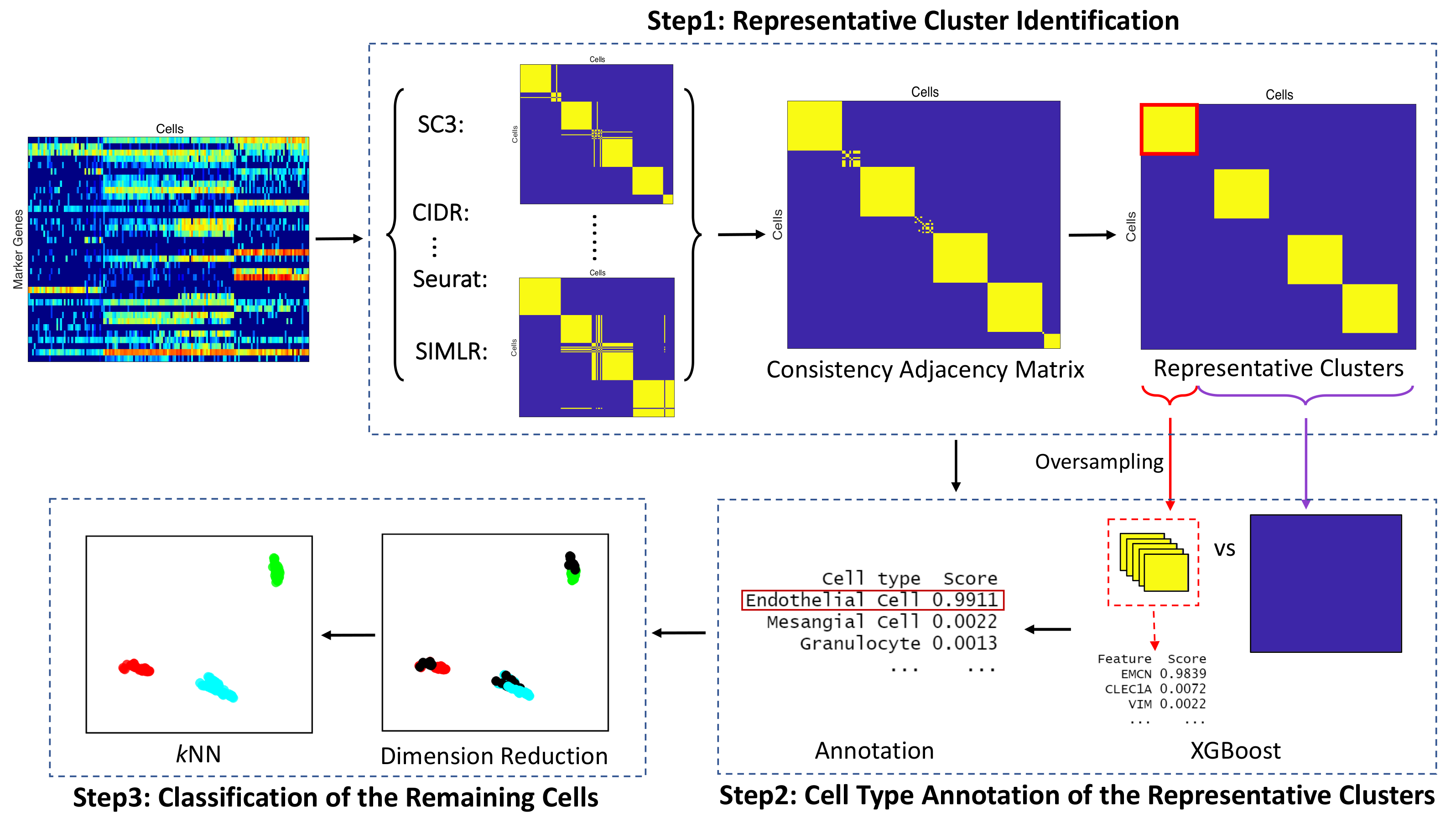
2.2. Methods
2.2.1. Representative Cluster Identification
2.2.2. Cell Type Annotation of the Representative Clusters
2.2.3. Classification of the Remaining Cells
| Algorithm 1 ACAM: Automatic Cell type Annotation Method. |
|
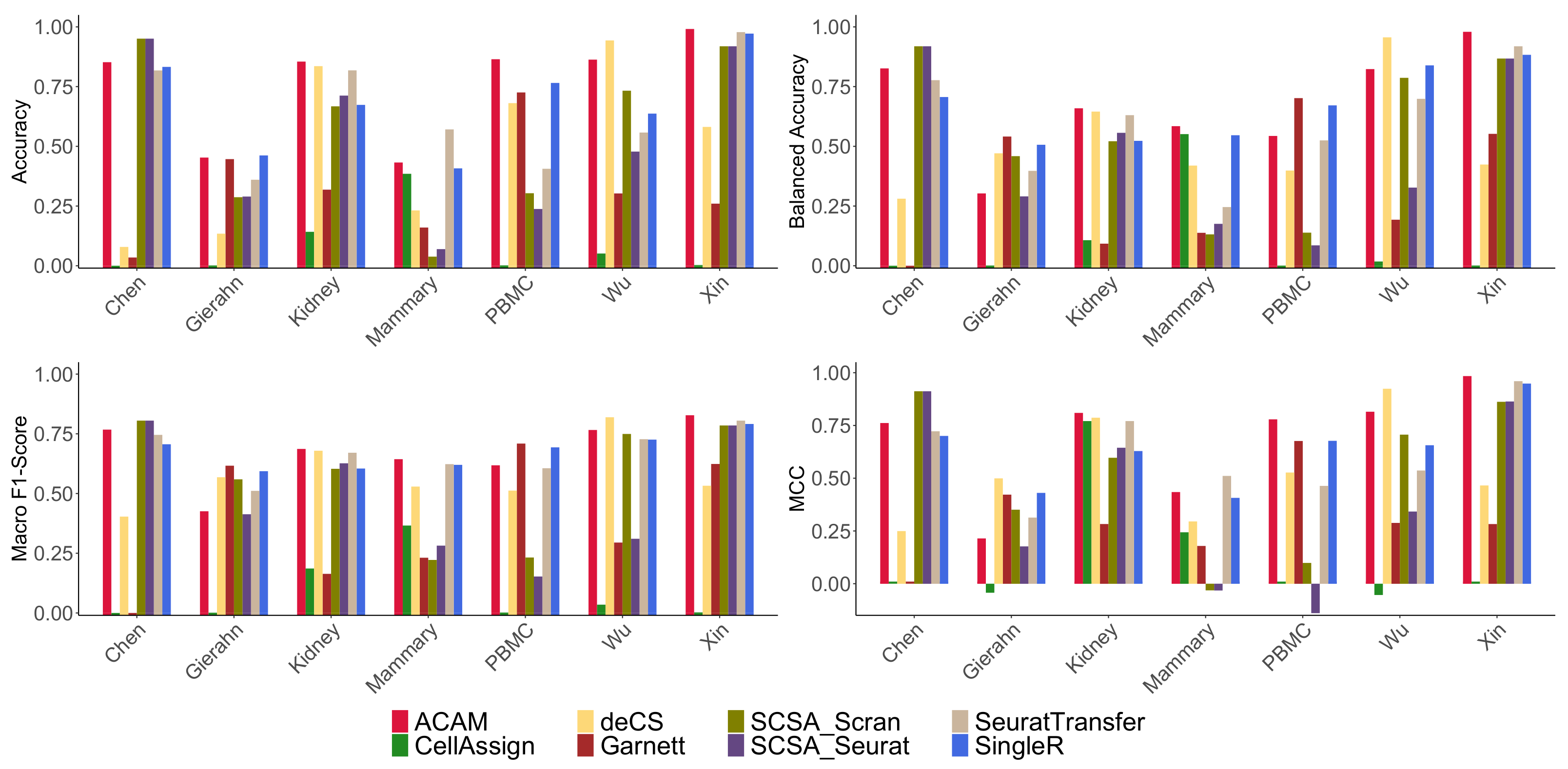
2.3. Results Evaluation Metrics
- Accuracy: It is defined as the percentage of true positives of the annotations:
- Balanced Accuracy: It is defined as the average Recall of each cell type,where
- Macro F1-Score: It is defined as the harmonic mean of average Precision and average Recall:where
- Matthews Correlation Coefficient (MCC): It takes into account the true and false positives and negatives and is generally regarded as a balanced measure which can be used even if the classes are of very different sizes:
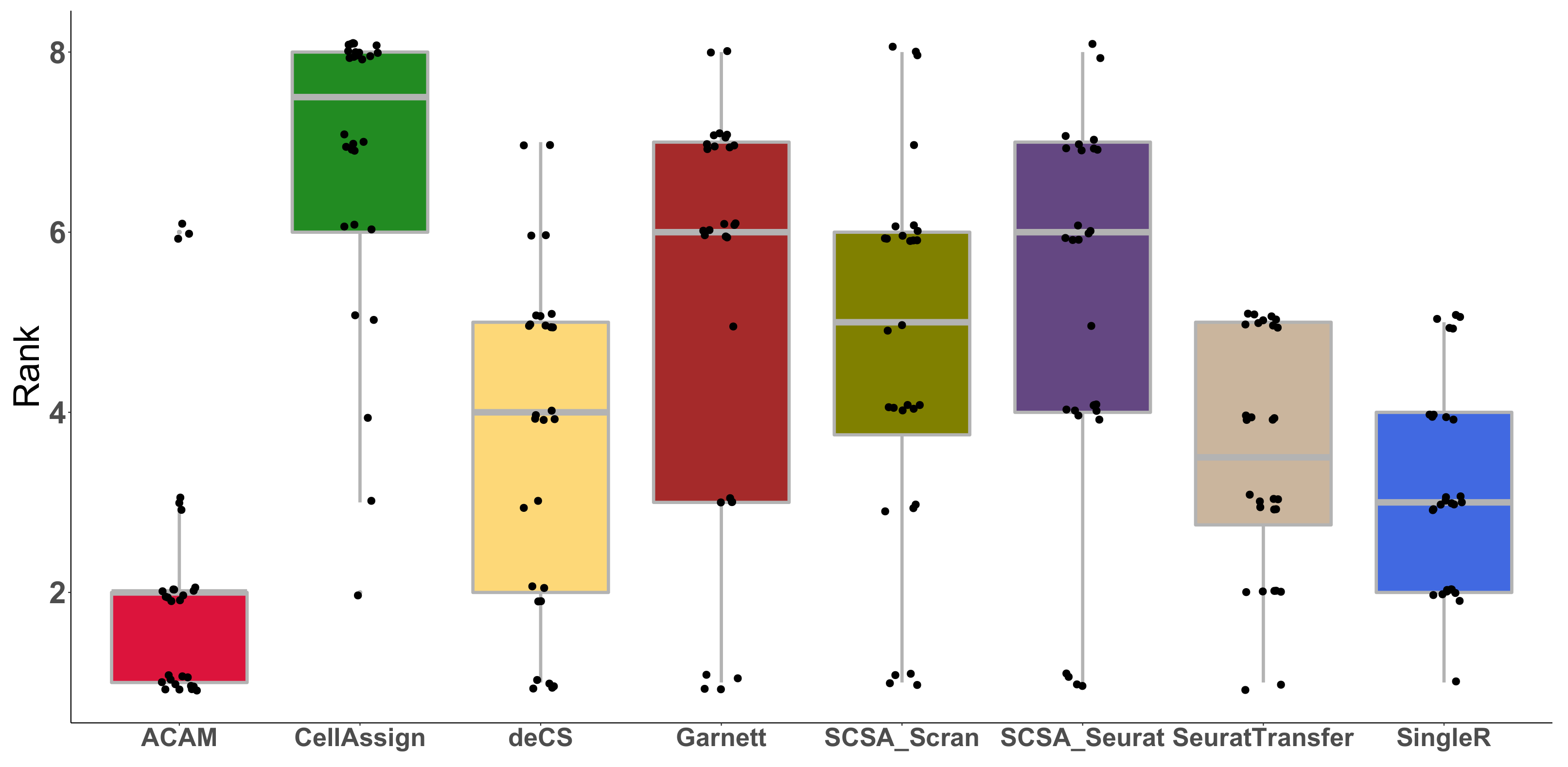
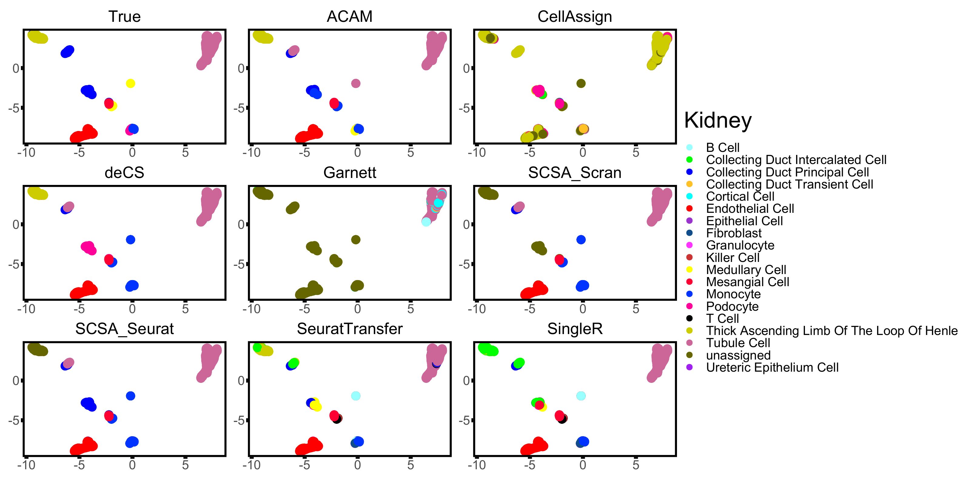
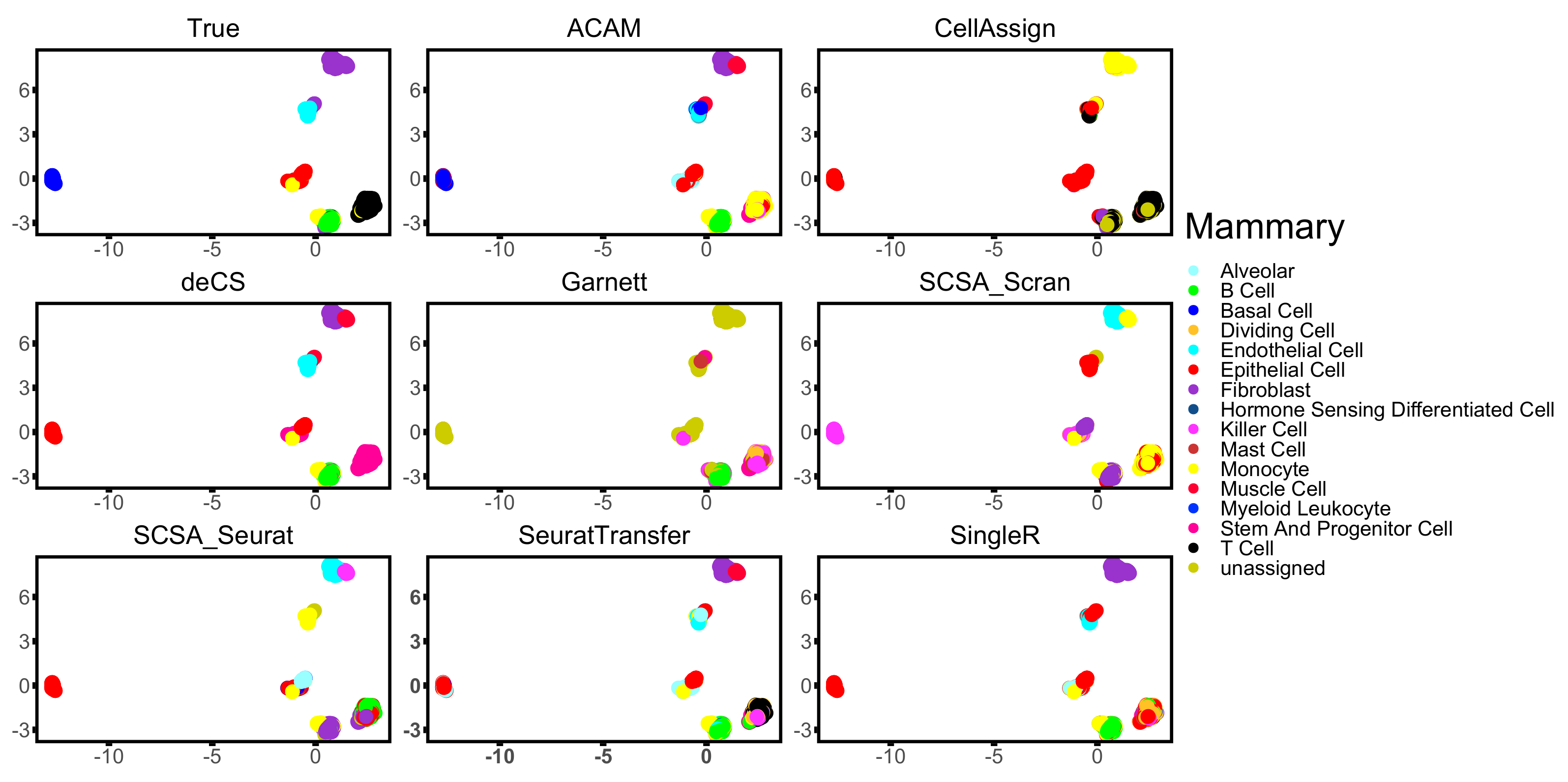
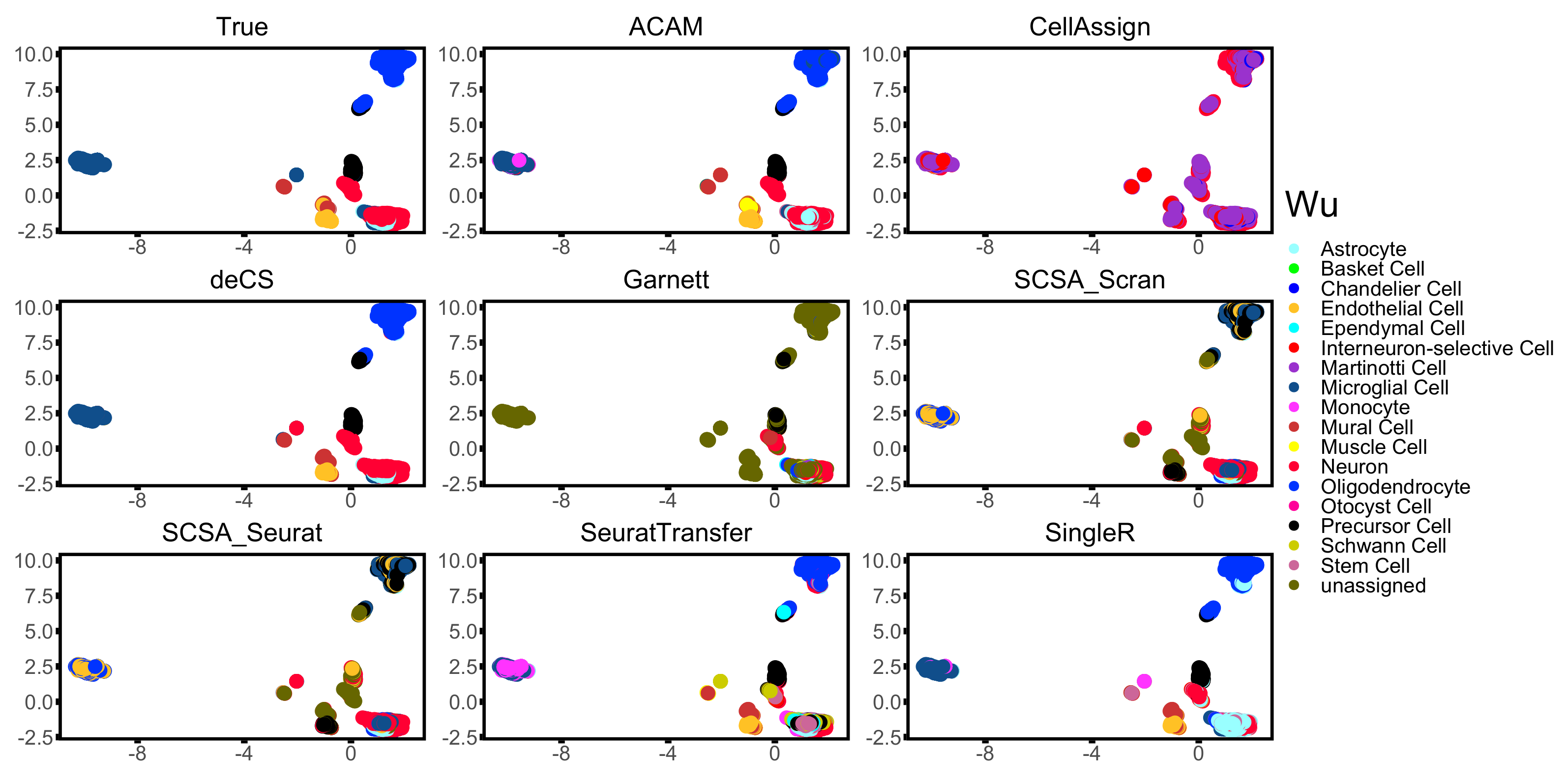
3. Results
3.1. Comparison Methods
- CellAssign It takes into account the prior knowledge of marker genes into a probabilistic model to estimate cell types with parameters selected by the maximum a posteriori probability, and google tensorflow is used in EM step.
- deCS It first conducts clustering by Seurat [26]. Differentially expressed genes of clusters are then extracted using function FindAllMarkers in R package Seurat. It then annotates clusters as the cell type with the maximum overlap between cell type markers and the differentially expressed genes.
- Garnett It first chooses representative cells by aggregating marker scores from the TF-IDF matrix, and then trains the logistic regression model with elastic net to classify the remaining cells, regarding the representative cells as training set.
- SCSA Similar to deCS, SCSA first conducts clustering by Seurat [26]. Differentially expressed genes of clusters are extracted using the function FindAllMarkers in R package Seurat (SCSA_Seurat) and the function findMarkers in R package Scran (SCSA_Scran). SCSA calculates cell type scores of each cluster by adding up re-scaled log2-based fold change values (LFC) of differentially expressed marker genes. Clusters are then annotated by the cell type with the highest cell type score.
- SeuratTransfer It uses the function TransferData in the R package Seurat. It is a strategy to ‘anchor’ datasets together. By placing both the annotated reference scRNA-seq dataset and the unannotated dataset in a shared low-dimensional space using canonical correlation analysis (CCA), pairwise correspondences between cells from both datasets are identified as anchors by mutual nearest neighbors (MNN). For each cell in the unannotated dataset, it is scored and annotated depending on the distances to anchors.
- SingleR It first calculates the Spearman coefficients on variable genes between each unannotated cell and the annotated ones of each type in the reference scRNA-seq data. The same procedure is iteratively performed using the cell types with top correlations in the previous step. The cell is annotated as the type that is left till the last round.
3.2. Methods’ Implementation Details
3.3. Results
4. Conclusions and Discussion
Author Contributions
Funding
Institutional Review Board Statement
Informed Consent Statement
Data Availability Statement
Conflicts of Interest
Appendix A
References
- Kolodziejczyk, A.A.; Kim, J.K.; Svensson, V.; Marioni, J.C.; Teichmann, S.A. The technology and biology of single-cell RNA sequencing. Mol. Cell 2015, 58, 610–620. [Google Scholar] [CrossRef] [PubMed] [Green Version]
- Friebel, E.; Kapolou, K.; Unger, S.; Núñez, N.G.; Utz, S.; Rushing, E.J.; Regli, L.; Weller, M.; Greter, M.; Tugues, S.; et al. Single-cell mapping of human brain cancer reveals tumor-specific instruction of tissue-invading leukocytes. Cell 2020, 181, 1626–1642. [Google Scholar] [CrossRef]
- Tirosh, I.; Izar, B.; Prakadan, S.M.; Wadsworth, M.H.; Treacy, D.; Trombetta, J.J.; Rotem, A.; Rodman, C.; Lian, C.; Murphy, G.; et al. Dissecting the multicellular ecosystem of metastatic melanoma by single-cell RNA-seq. Science 2016, 352, 189–196. [Google Scholar] [CrossRef] [PubMed] [Green Version]
- Wagner, J.; Rapsomaniki, M.A.; Chevrier, S.; Anzeneder, T.; Langwieder, C.; Dykgers, A.; Rees, M.; Ramaswamy, A.; Muenst, S.; Soysal, S.D.; et al. A single-cell atlas of the tumor and immune ecosystem of human breast cancer. Cell 2019, 177, 1330–1345. [Google Scholar] [CrossRef] [PubMed] [Green Version]
- Zheng, H.; Pomyen, Y.; Hernandez, M.O.; Li, C.; Livak, F.; Tang, W.; Dang, H.; Greten, T.F.; Davis, J.L.; Zhao, Y.; et al. Single-cell analysis reveals cancer stem cell heterogeneity in hepatocellular carcinoma. Hepatology 2018, 68, 127–140. [Google Scholar] [CrossRef] [PubMed] [Green Version]
- Li, L.; Guo, F.; Gao, Y.; Ren, Y.; Yuan, P.; Yan, L.; Li, R.; Lian, Y.; Li, J.; Hu, B.; et al. Single-cell multi-omics sequencing of human early embryos. Nat. Cell Biol. 2018, 20, 847–858. [Google Scholar] [CrossRef]
- Wagner, D.E.; Weinreb, C.; Collins, Z.M.; Briggs, J.A.; Megason, S.G.; Klein, A.M. Single-cell mapping of gene expression landscapes and lineage in the zebrafish embryo. Science 2018, 360, 981–987. [Google Scholar] [CrossRef] [Green Version]
- Alquicira-Hernandez, J.; Sathe, A.; Ji, H.P.; Nguyen, Q.; Powell, J.E. scPred: Accurate supervised method for cell-type classification from single-cell RNA-seq data. Genome Biol. 2019, 20, 1–17. [Google Scholar] [CrossRef] [Green Version]
- Aran, D.; Looney, A.P.; Liu, L.; Wu, E.; Fong, V.; Hsu, A.; Chak, S.; Naikawadi, R.P.; Wolters, P.J.; Abate, A.R.; et al. Reference-based analysis of lung single-cell sequencing reveals a transitional profibrotic macrophage. Nat. Immunol. 2019, 20, 163–172. [Google Scholar] [CrossRef]
- Brbić, M.; Zitnik, M.; Wang, S.; Pisco, A.O.; Altman, R.B.; Darmanis, S.; Leskovec, J. MARS: Discovering novel cell types across heterogeneous single-cell experiments. Nat. Methods 2020, 12, 1200–1206. [Google Scholar] [CrossRef]
- Hou, R.; Denisenko, E.; Forrest, A.R. scMatch: A single-cell gene expression profile annotation tool using reference datasets. Bioinformatics 2019, 35, 4688–4695. [Google Scholar] [CrossRef] [PubMed] [Green Version]
- Hu, J.; Li, X.; Hu, G.; Lyu, Y.; Susztak, K.; Li, M. Iterative transfer learning with neural network for clustering and cell type classification in single-cell RNA-seq analysis. Nat. Mach. Intell. 2020, 2, 607–618. [Google Scholar] [CrossRef] [PubMed]
- De Kanter, J.K.; Lijnzaad, P.; Candelli, T.; Margaritis, T.; Holstege, F.C. CHETAH: A selective, hierarchical cell type identification method for single-cell RNA sequencing. Nucleic Acids Res. 2019, 47, e95. [Google Scholar] [CrossRef] [PubMed] [Green Version]
- Kiselev, V.Y.; Yiu, A.; Hemberg, M. scmap: Projection of single-cell RNA-seq data across data sets. Nat. Methods 2018, 15, 359–362. [Google Scholar] [CrossRef] [PubMed]
- Pasquini, G.; Arias, J.E.R.; Schäfer, P.; Busskamp, V. Automated methods for cell type annotation on scRNA-seq data. Comput. Struct. Biotechnol. J. 2021, 19, 961–969. [Google Scholar] [CrossRef]
- Pliner, H.A.; Shendure, J.; Trapnell, C. Supervised classification enables rapid annotation of cell atlases. Nat. Methods 2019, 16, 983–986. [Google Scholar] [CrossRef]
- Shao, X.; Liao, J.; Lu, X.; Xue, R.; Ai, N.; Fan, X. scCATCH: Automatic annotation on cell types of clusters from single-cell RNA sequencing data. Iscience 2020, 23, 100882. [Google Scholar] [CrossRef] [Green Version]
- Shao, X.; Yang, H.; Zhuang, X.; Liao, J.; Yang, P.; Cheng, J.; Lu, X.; Chen, H.; Fan, X. scDeepSort: A pre-trained cell-type annotation method for single-cell transcriptomics using deep learning with a weighted graph neural network. Nucleic Acids Res. 2021. [Google Scholar] [CrossRef]
- Zhang, A.W.; Oflanagan, C.H.; Chavez, E.A.; Lim, J.L.P.; Ceglia, N.; Mcpherson, A.; Wiens, M.; Walters, P.; Chan, T.M.; Hewitson, B.; et al. Probabilistic cell-type assignment of single-cell RNA-seq for tumor microenvironment profiling. Nat. Methods 2019, 16, 1007–1015. [Google Scholar] [CrossRef]
- Pei, G.; Yan, F.; Simon, L.M.; Dai, Y.; Jia, P.; Zhao, Z. deCS: A tool for systematic cell type annotations of single-cell RNA sequencing data among human tissues. Genom. Proteom. Bioinform. 2022, 22. [Google Scholar] [CrossRef]
- Stuart, T.; Butler, A.; Hoffman, P.; Hafemeister, C.; Papalexi, E.; Mauck III, W.M.; Hao, Y.; Stoeckius, M.; Smibert, P.; Satija, R. Comprehensive integration of single-cell data. Cell 2019, 177, 1888–1902. [Google Scholar] [CrossRef]
- Wei, Z.; Zhang, S. CALLR: A semi-supervised cell-type annotation method for single-cell RNA sequencing data. Bioinformatics 2021, 37, i51–i58. [Google Scholar] [CrossRef]
- DePasquale, E.A.; Schnell, D.; Dexheimer, P.; Ferchen, K.; Hay, S.; Chetal, K.; Valiente-Alandí, Í.; Blaxall, B.C.; Grimes, H.L.; Salomonis, N. cellHarmony: Cell-level matching and holistic comparison of single-cell transcriptomes. Nucleic Acids Res. 2019, 47, e138. [Google Scholar] [CrossRef] [Green Version]
- Seal, D.B.; Das, V.; De, R.K. CASSL: A cell-type annotation method for single cell transcriptomics data using semi-supervised learning. Appl. Intell. 2022. [Google Scholar] [CrossRef]
- Cao, Y.; Wang, X.; Peng, G. SCSA: A cell type annotation tool for single-cell RNA-seq data. Front. Genet. 2020, 11, 490. [Google Scholar] [CrossRef]
- Butler, A.; Hoffman, P.J.; Smibert, P.; Papalexi, E.; Satija, R. Integrating single-cell transcriptomic data across different conditions, technologies, and species. Nat. Biotechnol. 2018, 36, 411–420. [Google Scholar] [CrossRef]
- Kiselev, V.Y.; Kirschner, K.; Schaub, M.T.; Andrews, T.S.; Yiu, A.; Chandra, T.; Natarajan, K.N.; Reik, W.; Barahona, M.; Green, A.R.; et al. SC3: Consensus clustering of single-cell RNA-seq data. Nat. Methods 2017, 14, 483–486. [Google Scholar] [CrossRef] [Green Version]
- Lin, P.; Troup, M.; Ho, J.W.K. CIDR: Ultrafast and accurate clustering through imputation for single-cell RNA-seq data. Genome Biol. 2017, 18, 59. [Google Scholar] [CrossRef] [Green Version]
- Van der Maaten, L.; Hinton, G. Visualizing data using t-SNE. J. Mach. Learn. Res. 2008, 9, 2579–2605. [Google Scholar]
- Wang, B.; Zhu, J.; Pierson, E.; Ramazzotti, D.; Batzoglou, S. Visualization and analysis of single-cell RNA-seq data by kernel-based similarity learning. Nat. Methods 2017, 14, 414–416. [Google Scholar] [CrossRef]
- Chen, L.; Lee, J.W.; Chou, C.L.; Nair, A.V.; Battistone, M.A.; Păunescu, T.G.; Merkulova, M.; Breton, S.; Verlander, J.W.; Wall, S.M.; et al. Transcriptomes of major renal collecting duct cell types in mouse identified by single-cell RNA-seq. Proc. Natl. Acad. Sci. USA 2017, 114, E9989–E9998. [Google Scholar] [CrossRef]
- Xin, Y.; Kim, J.; Okamoto, H.; Ni, M.; Wei, Y.; Adler, C.; Murphy, A.J.; Yancopoulos, G.D.; Lin, C.; Gromada, J. RNA sequencing of single human islet cells reveals type 2 diabetes genes. Cell Metab. 2016, 24, 608–615. [Google Scholar] [CrossRef] [Green Version]
- Tabula Muris Consortium. Single-cell transcriptomics of 20 mouse organs creates a Tabula Muris. Nature 2018, 562, 367–372. [Google Scholar] [CrossRef]
- Gierahn, T.M.; Wadsworth, M.H.; Hughes, T.K.; Bryson, B.D.; Butler, A.; Satija, R.; Fortune, S.; Love, J.C.; Shalek, A.K. Erratum: Seq-Well: Portable, low-cost RNA sequencing of single cells at high throughput. Nat. Methods 2017, 14, 752. [Google Scholar] [CrossRef] [Green Version]
- Wu, Y.E.; Pan, L.; Zuo, Y.; Li, X.; Hong, W. Detecting activated cell populations using single-cell RNA-seq. Neuron 2017, 96, 313–329. [Google Scholar] [CrossRef] [PubMed] [Green Version]
- Zeisel, A.; Hochgerner, H.; Lönnerberg, P.; Johnsson, A.; Memic, F.; Van Der Zwan, J.; Häring, M.; Braun, E.; Borm, L.E.; La Manno, G.; et al. Molecular architecture of the mouse nervous system. Cell 2018, 174, 999–1014. [Google Scholar] [CrossRef] [PubMed] [Green Version]
- Zhang, X.; Lan, Y.; Xu, J.; Quan, F.; Zhao, E.; Deng, C.; Luo, T.; Xu, L.; Liao, G.; Yan, M.; et al. CellMarker: A manually curated resource of cell markers in human and mouse. Nucleic Acids Res. 2019, 47, D721–D728. [Google Scholar] [CrossRef] [PubMed] [Green Version]
- Han, X.; Wang, R.; Zhou, Y.; Fei, L.; Sun, H.; Lai, S.; Saadatpour, A.; Zhou, Z.; Chen, H.; Ye, F.; et al. Mapping the mouse cell atlas by microwell-seq. Cell 2018, 172, 1091–1107. [Google Scholar] [CrossRef] [Green Version]
- Yuan, H.; Yan, M.; Zhang, G.; Liu, W.; Deng, C.; Liao, G.; Xu, L.; Luo, T.; Yan, H.; Long, Z.; et al. CancerSEA: A cancer single-cell state atlas. Nucleic Acids Res. 2019, 47, D900–D908. [Google Scholar] [CrossRef] [Green Version]
- BD Biosciences. CD Marker Handbook. Available online: http://static.bdbiosciences.com/documents/cd_marker_handbook.pdf (accessed on 15 August 2022).
- Hao, Y.; Hao, S.; Andersen-Nissen, E.; Mauck, W.M., III; Zheng, S.; Butler, A.; Lee, M.J.; Wilk, A.J.; Darby, C.; Zager, M.; et al. Integrated analysis of multimodal single-cell data. Cell 2021, 184, 3573–3587. [Google Scholar] [CrossRef]
- Huh, R.; Yang, Y.; Jiang, Y.; Shen, Y.; Li, Y. SAME-clustering: Single-cell Aggregated Clustering via Mixture Model Ensemble. Nucleic Acids Res. 2020, 48, 86–95. [Google Scholar] [CrossRef]
- Hubert, L.; Arabie, P. Comparing partitions. J. Classif. 1985, 2, 193–218. [Google Scholar] [CrossRef]
- Blondel, V.D.; Guillaume, J.L.; Lambiotte, R.; Lefebvre, E. Fast unfolding of communities in large networks. J. Stat. Mech. Theory Exp. 2008, 2008, P10008. [Google Scholar] [CrossRef] [Green Version]
- Chen, T.; He, T.; Benesty, M.; Khotilovich, V.; Tang, Y.; Cho, H.; Chen, K. Xgboost: Extreme gradient boosting. R Package Version 0.4-2 2015, 1, 1–4. [Google Scholar]
- McInnes, L.; Healy, J.; Melville, J. UMAP: Uniform Manifold Approximation and Projection for Dimension Reduction. Stat 2020, 1050, 18. [Google Scholar]
- Grandini, M.; Bagli, E.; Visani, G. Metrics for multi-class classification: An overview. arXiv 2020, arXiv:2008.05756. [Google Scholar]
- Lun, A.T.; McCarthy, D.J.; Marioni, J.C. A step-by-step workflow for low-level analysis of single-cell RNA-seq data with Bioconductor. F1000Research 2016, 5, 2122. [Google Scholar] [CrossRef] [Green Version]


| Dataset | Platform | Samples | Cell Types | Species | Tissue |
|---|---|---|---|---|---|
| Chen [31] | Fluidigm C1 system | 203 | 3 | Mouse | Kidney |
| Xin [32] | Fluidigm C1 system | 1600 | 4 | Human | Pancreatic Islet |
| Gierahn [34] | Seqwell | 3694 | 5 | Human | Peripheral Blood |
| Wu [35] | DropSeq | 20,679 | 7 | Mouse | Brain |
| PBMC [26] | 10× | 2638 | 4 | Human | Peripheral Blood |
| Kidney [33] | 10× | 2781 | 8 | Mouse | Kidney |
| Mammary [33] | 10× | 4481 | 7 | Mouse | Mammary Gland |
Publisher’s Note: MDPI stays neutral with regard to jurisdictional claims in published maps and institutional affiliations. |
© 2022 by the authors. Licensee MDPI, Basel, Switzerland. This article is an open access article distributed under the terms and conditions of the Creative Commons Attribution (CC BY) license (https://creativecommons.org/licenses/by/4.0/).
Share and Cite
Chen, Y.; Zhang, S. Automatic Cell Type Annotation Using Marker Genes for Single-Cell RNA Sequencing Data. Biomolecules 2022, 12, 1539. https://doi.org/10.3390/biom12101539
Chen Y, Zhang S. Automatic Cell Type Annotation Using Marker Genes for Single-Cell RNA Sequencing Data. Biomolecules. 2022; 12(10):1539. https://doi.org/10.3390/biom12101539
Chicago/Turabian StyleChen, Yu, and Shuqin Zhang. 2022. "Automatic Cell Type Annotation Using Marker Genes for Single-Cell RNA Sequencing Data" Biomolecules 12, no. 10: 1539. https://doi.org/10.3390/biom12101539