

Photoionization and Electron–Ion Recombination in Astrophysical Plasmas

Department of Physics and Astronomy & Pittsburgh Particle Physics, Astrophysics and Cosmology Center (PITT PACC), University of Pittsburgh, 3941 O’Hara Street, Pittsburgh, PA 15260, USA
Atoms 2023, 11(3), 54; https://doi.org/10.3390/atoms11030054
Submission received: 24 January 2023
/
Revised: 3 March 2023
/
Accepted: 3 March 2023
/
Published: 9 March 2023
(This article belongs to the Special Issue Photoionization of Atoms)
Abstract
:Photoionization and its inverse, electron–ion recombination, are key processes that influence many astrophysical plasmas (and gasses), and the diagnostics that we use to analyze the plasmas. In this review we provide a brief overview of the importance of photoionization and recombination in astrophysics. We highlight how the data needed for spectral analyses, and the required accuracy, varies considerably in different astrophysical environments. We then discuss photoionization processes, highlighting resonances in their cross-sections. Next we discuss radiative recombination, and low and high temperature dielectronic recombination. The possible suppression of low temperature dielectronic recombination (LTDR) and high temperature dielectronic recombination (HTDR) due to the radiation field and high densities is discussed. Finally we discuss a few astrophysical examples to highlight photoionization and recombination processes.
1. Introduction
One of the most important ways we learn about the Universe is through spectroscopy. From spectroscopy we can typically deduce important stellar parameters such as a star’s effective temperature,1 surface gravity (=) and abundances. These in turn provide insights into stellar evolution, galactic evolution, and the evolution of the Universe. To perform analyses of stellar data requires atomic data, although the amount and type of atomic data needed varies greatly with the application. In the most extreme cases, in which local thermodynamic equilibrium does not hold (discussed below), we require, for example, photoionization cross-sections, oscillator strengths for bound–bound transitions, line-broadening data, collisional cross-sections, autoionization rates, chemical reaction rates, and charge exchange cross-sections. For some simple species, such as hydrogen, we have excellent atomic data while for other important species, such as Fe group elements, crucial atomic data is lacking. Unfortunately, for many ionization stages even basic information, such as accurate energy levels, is also missing.2 However, invaluable work by the NIST and Imperial college atomic spectroscopy groups is helping to rectify this situation for some important astrophysical ions (e.g., [2,3]).
In this review we discuss the importance of photoionization cross-sections for astronomical applications, with an emphasis on massive stars. Such a discussion will necessarily consider recombination processes—the inverse of photoionization processes. Before doing so it is necessary to define some important physical and astronomical terms.
A star (or any other astrophysical object emitting radiation) is not in thermal equilibrium. However, in some cases, and at some locations, it is well justified to assume that the plasma in the star is in “local” thermal equilibrium. Below the atmosphere (the thin layer that emits the radiation we observe) the material in most stars can be considered to be in “local” thermal equilibrium (LTE). In such cases, the state of the gas (e.g., the thermodynamical properties, the ionization state, and the populations of atomic levels) are set by the density and electron temperature via thermodynamic arguments. The ionization state of the gas and the level populations are determined, for example, by the Saha and Boltzmann equations (e.g., [4]). Moreover, there is only one temperature—the electron temperature, the ion temperature, the excitation temperature, and the radiation temperature are all identical. The temperature of the gas varies with location (it must, since radiation is propagating outwards) but the scale on which it varies does not affect the thermodynamic state of the gas. Unfortunately, much of the radiation we observe comes from gas that is NOT in LTE—typically referred to as nLTE or non-LTE.
At the stellar surface the assumption of LTE becomes less valid. This is not surprising—at the stellar surface radiation is escaping from the star and there is no incident radiation (at least for single stars), and hence the radiation density must drop from its blackbody value by a factor of (at least) ∼2 (since there is no incident radiation—see (see [4], p. 120). Further, because radiation can now travel significant distances, regions of different temperatures are directly coupled, potentially making the radiation field at a given location strongly non-Planckian.
Fortunately, in some cases the densities are high enough that collisional processes can still strongly couple the level populations and the ionization state of the gas to the local electron temperature, allowing us to use the Saha and Boltzmann equations to compute level populations. In such cases the electron temperature (which will be the same as the ion temperature) determines the state of the gas and it is this temperature that we normally state. In general, however, the electron and radiation temperatures will be different.3
The Boltzmann equation, which relates the populations of two levels within the same ionization state, is
where and are the LTE population densities of the lower and upper states, respectively, and are the level degeneracies, and is the difference energy between the two levels (e.g., [4]).
The Saha equation, which relates the ground state populations of two consecutive ionization equations, is
where T is the electron temperature in Kelvin, (cgs units), is the electron density, is the ionization energy, and the subscript i () is used to denote the ionization stage.
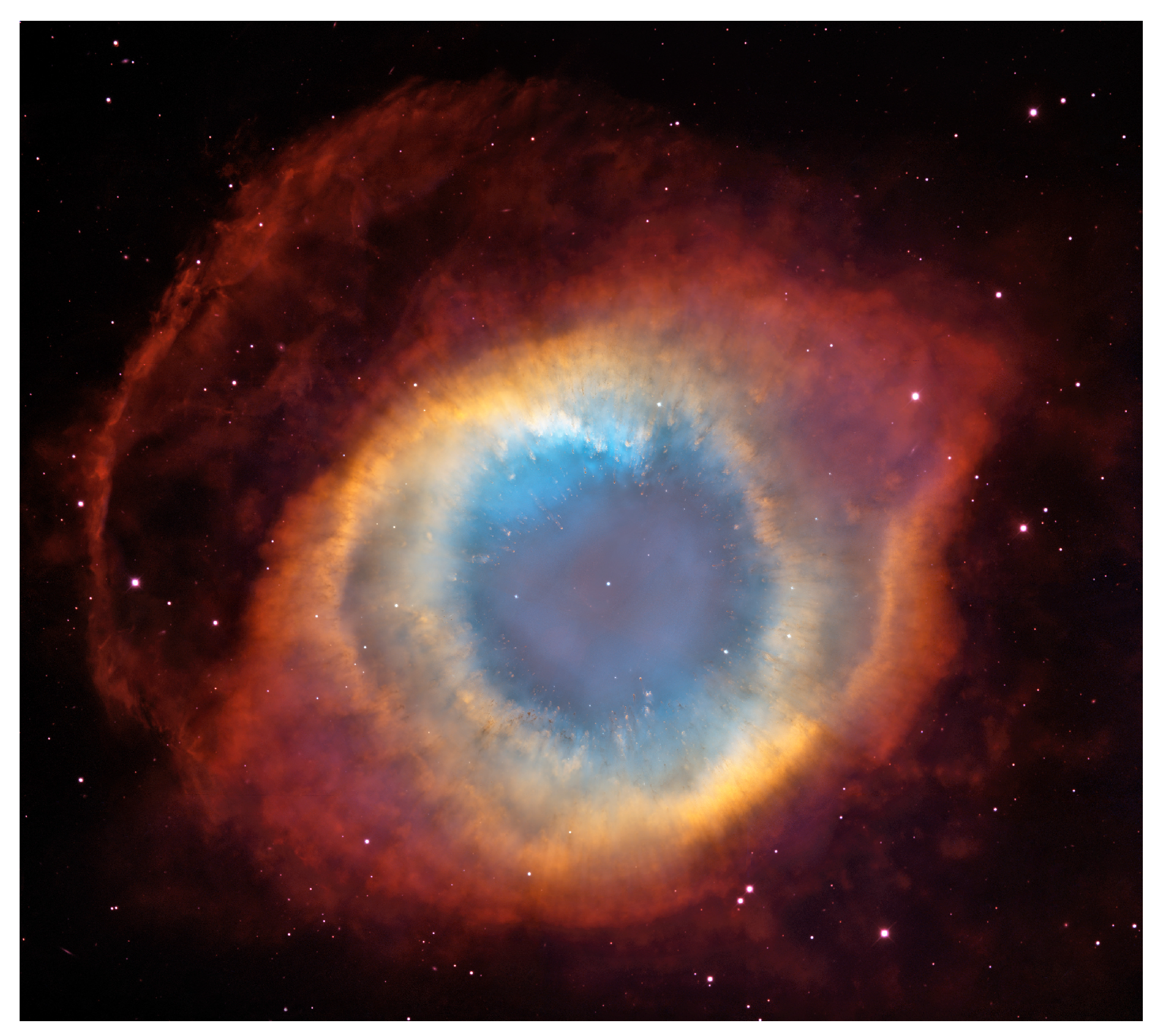
In many stars, and especially those with lower density gas (nebulae, stellar winds, supernovae) the departures from LTE are significant and MUST be allowed for. Gaseous nebulae, which typically have densities less than atoms cm, provide an excellent example in which the departures from LTE are extreme. The radiation field that ionizes the nebula typically emanates from a hot star (K) and is strongly diluted since the nebula is typically very distant from the star (Figure 1). The equilibrium temperature of the gas is typically around 10,000 K (which is primarily determined by the chemical composition of the nebula) and is insensitive to the effective temperature of the star. The nebula, longward (i.e., at larger wavelengths) of the H i Lyman jump at 912 Å, is transparent to most radiation. Because of the non-Planckian radiation field and the low densities, collisions with electrons cannot drive the gas into LTE.
When LTE no longer holds (i.e., nLTE) we are forced to solve for the ionization state of the gas and the level populations from first principles. That is, we need to consider all the processes, and inverse processes, that populate a given level. These processes include photoionization and recombination, bound–bound emission and absorption, collisional excitation and de-excitation, collisional ionization and collisional recombination, dielectronic recombination and autoionization, charge exchange reactions and, in “cooler gas” ( K), chemical reactions, and dust chemistry.4 Determining the state of the gas is a complicated problem. Many of the processes above depend on the radiation field which in turn depends on the level populations. Further, the radiation field couples the gas to regions of different temperatures. This is a highly non-linear problem and can only be solved by iterative techniques. In many cases we can consider the population numbers to be static (and the equations are referred to as the equations of statistical equilibrium) but in other cases (e.g., supernovae) we may need to allow for time dependence (and solve the kinetic equations). Another major issue is correcting for plasma effects that limit the number of levels in atoms and ions (i.e., crudely, an atom/ion cannot be larger than the inter-atom spacing). One approach is probabilistic and was developed in a series of papers by Hummer, Mihalas, and Dappen [12,13,14], and is used, for example, in the nLTE radiative transfer codes tlusty [15] and cmfgen [16]. In this approach, levels are assigned an occupation probability that varies smoothly with the level energy, density and temperature, and that leads to a finite partition function.
Thus, a vast amount of atomic data is needed. Sadly, despite heroic efforts by Bob Kurucz [17,18], members of the Opacity Project [19] and Iron Project [20], Sultana Nahar [21], and many others, much of the needed data is still missing. Extensive photoionization data is available, for example, through TOPbase [22], TIPbase [23], and NORAD [21]. As discussed later in this article, details can matter, and it is not always obvious, a priori, which data are essential for accurate analyses. As this paper is concerned with photoionization/recombination, this paper does not generally elaborate on other important processes. Information on these additional processes can be found in, e.g., [24,25,26,27].
Below we discuss photoionization and recombination as relevant to astrophysical applications. Much of the following discussion will be based on my own experiences in developing cmfgen, a nLTE radiative transfer code originally designed to model hot massive stars K) and their stellar winds [16,28]. The winds in these stars are driven by radiation pressure acting on bound–bound transitions belonging, for example, to C, N, O, Ar, and Fe (e.g., [29,30,31]). Since its initial development the code has undergone considerable revisions and improvements. It has been successfully used to model O stars (e.g., [32,33,34,35,36]), Wolf–Rayet (WR) stars [37,38], luminous blue variables (e.g., [39,40,41]), B stars (e.g., [42]), the central stars of planetary nebulae (e.g., [43]), and A stars. Over the last decade cmfgen was adapted to treat time-dependent radiation transfer, and to solve the time-dependent kinetic equations [44], and it has been used to model spectra resulting from a variety of SN explosions (e.g., [45,46,47,48]).
The review is organized as follows: In Section 2 we briefly discuss the importance of photoionization processes for stellar interiors and introduce the Rosseland mean opacity. We then consider photoionization processes in Section 3 with an emphasis on inner shell ionizations in Section 3.1. Recombination processes are discussed in Section 4 while suppression of dielectronic recombination by collisions and the radiation field is discussed in Section 5.1 and Section 5.2 respectively. Specific examples of where photoionization/recombination processes are important are then discussed—direct recombination (Section 6.1), the Sun (Section 6.2), O stars, WR stars, luminous blue variables (LBVs), (Section 6.3), Of and WN stars (Section 6.3.1), carbon lines in WC stars (Section 6.3.2), C ii in a [WC] star (Section 6.4), and supernovae (Section 6.5).
2. Stellar Interiors
In stellar interiors energy is transported by radiation and by convection, and in degenerate stars by conduction. As LTE holds, photoionization processes have no direct influence on the level populations (since the populations are determined by the Saha and Boltzmann equations), but they do help to determine the temperature of the gas and they do help to set the continuous radiation field that we observe. Due to the small mean-free-path of photons, radiation transport is diffusive and in this regime a single quantity, the Rosseland mean opacity, is required to describe the transport of radiative energy. At depth in the star the radiation diffuses and the specific intensity () at frequency is given by
(e.g., [4]) where is the Planck (i.e., blackbody) function given by
is the opacity, and is the angle between the radius and the direction of radiation propagation. The radiative flux is simply given by
The negative sign in the expression for the flux arises because T, and hence , decrease with increasing r. Integrating over all frequencies yields a total radiative flux, F, given by
where is the Stefan–Boltzmann constant and is the Rosseland mean opacity as defined by
In stellar interiors the Rosseland mean opacity is a function of density, temperature, and composition, and is primarily determined by the most abundant species, with H, He, C, N, O, Ne, and Fe being the most crucial. As it is a harmonic mean it can be strongly influenced by regions of low opacity. Thus, it is crucial to take into account all opacity sources, particularly contributions in regions of otherwise low opacity. For a given species, the opacity is determined by photo-ionization processes, bound–bound transitions, and free–free processes. The required cross-sections are non-trivial to compute, especially for Fe group elements (with a partial filled 3d shell). Fortunately, because it is a broad integral, the Rosseland mean opacity is insensitive to small random errors (e.g., bound–bound transitions slightly offset from their correct wavelength) in the atomic data.
The computation of the Rosseland mean opacity is further complicated by the need to account for plasma effects—atoms/ions in a star are not isolated but experience a time-varying electric field due to their neighbors. This broadens bound–bound transitions which enhances the Rosseland mean opacity since the influence of the line is spread over a broader band into regions which may have lower opacity. Further, the size of the atoms/ions (and hence the number of levels) will be truncated since atoms/ions can only occupy a finite volume. The latter can be thought of as a lowering of the ionization potential but more rigorous approaches, for example, use probabilistic arguments [12,49]. An extensive discussion of some of the issues related to plasma effects on the equation of state, and additional references, are given by [50]. Extensive efforts have been made to provide LTE opacity libraries for stellar astrophysics that take into account different physical effects with varying degrees of fidelity. These include the Opacity Project [51], opacities computed using the opal code (e.g., [52,53]), the opas code [54], and a suite of codes developed at The Los Alamos National Laboratory [55].
3. Photoionization
The photoionization rate from a level l (in an arbitrary ion of arbitrary charge) can be written as
where is the population density of level l, is the frequency dependent photoionization cross-section (units are cm), the threshold frequency for ionization, h is Planck’s constant, and is the mean intensity (erg cm s Hz). is defined by
where is an increment in solid angle. If the radiation field is Planckian and isotropic,
The photoionization cross-sections are generally obtained from numerical calculations —it is not feasible to measure all the cross-sections in the laboratory. Rather, laboratory measurements are used to test the accuracy of theoretical calculations. The accuracy of the cross-section varies greatly being dependent on both assumptions used in the modeling and on the complexity of the model atom. For example, it is much easier to compute atomic data for atoms/ions with a partially filled p shell than it is for the lanthanides and actinides which have a partially filled 4f or 5f shell, respectively (e.g., [56]). The lanthanides are believed to be created in neutron–neutron star mergers and are an important opacity source in the outburst spectra that result from such mergers [57,58,59,60,61,62].
Typically in model atmosphere codes the rates (integrals) are evaluated using numerical quadrature. Thus
where is the quadrature weight at frequency .
In a simple species such as hydrogen, the photoionization process is simply
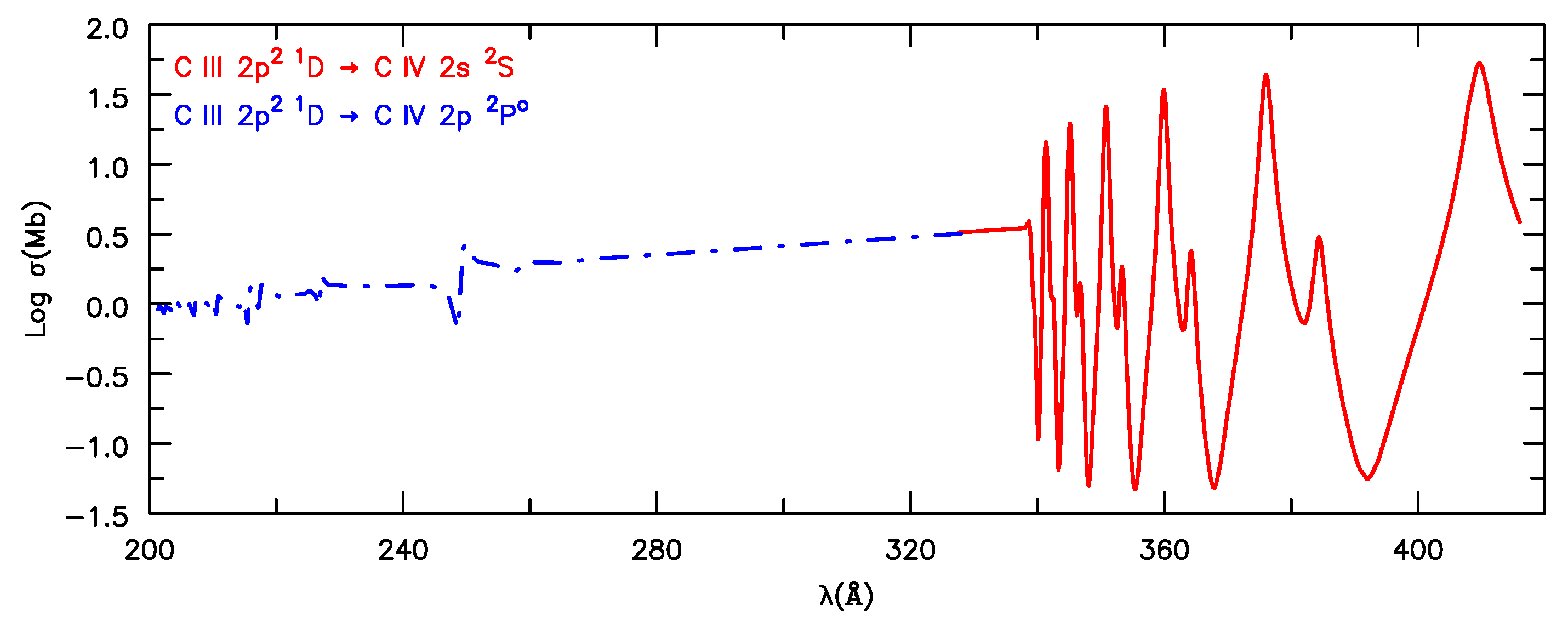
In more electron-rich species the process is more complicated since there are multiple photoionization routes. For example, there are two direct photoionization routes from C iii(2s 2p):
The first process occurs provided the photon energy exceeds the ionization energy of the C iii(2s 2p 1Po) state5. The second process occurs when the photon energy exceeds the sum of the ionization energy and the difference in energy between the 2s and 2p states in C iv. Of course, photons of sufficient energy may also ionize C by ejecting an inner (1s) electron—a process of great importance when X-rays are present.
There may also be multiple indirect photoionization routes such as:
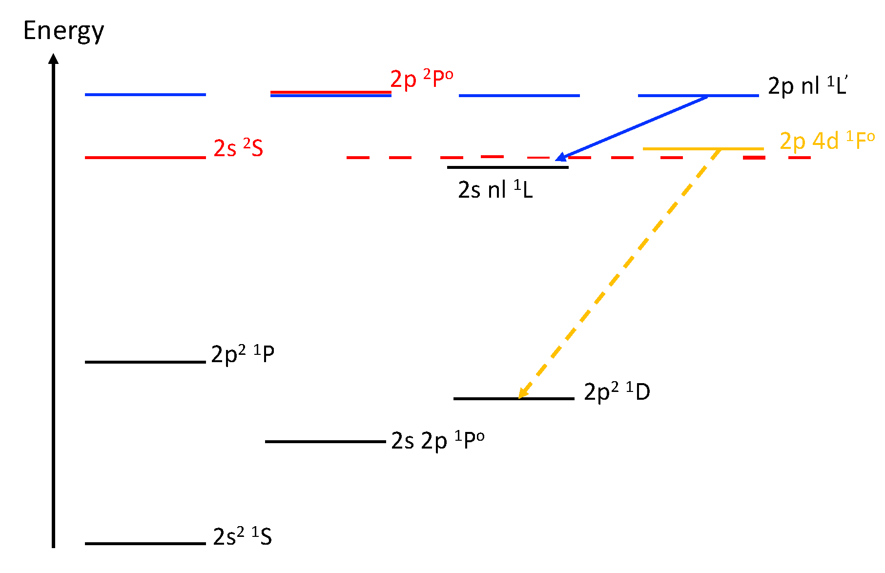
The above produces a relatively “narrow” resonance in the photoionization cross-section—it is narrow since the photon has to have the right energy to excite one of the 2p electrons into the 4d state (Figure 2). The energy of this state lies above the C iv ground state. The last step in this process is referred to as autoionization.
In LTE the final state arising from the photoionization process is irrelevant—only the total opacity matters. In general, in nLTE, the final state matters, since each process contributes to the population of a different state whose population needs to be determined from first principles. In practice this is generally not a crucial concern for most spectral modeling since the rates for processes connecting states within an ion are generally much larger than the photoionization and recombination rates. However, there are cases where the final-state-dependent cross-sections are important.
As a first example, we again consider the C iii / C iv system in WR stars6. In the photosphere the strong C iv doublet (due to 1 2s–1 2p) is optically thick, and hence the 1 2p state is strongly coupled to the 1 2s ground state through collisional de-excitation and excitation (i.e., the 2p state is in LTE (computed using the local electron temperature) with respect to the 2s state). Consequently we can treat all ionizations/recombinations as occurring to/from the C iv ground state. However, as the density declines photon escape in the resonance line will lead to a decoupling of 1 2p from the 1 2s state, in which case we should treat recombinations from the 1 2p state separately from those occurring from the 1 2s state. Fortunately, because the 1 2p state lies eV above the ground state, recombinations from the 1 2p state are generally not very important for the temperatures and densities appropriate to WR stars in the regime important for spectrum formation. This may not be the case in other regimes, and for other ions with states closer in energy to the ground state.
One crucial area where state-dependent photoionization cross-sections are important is in X-ray fluorescence where the ejection of an inner shell electron leads to the ion being in a highly excited state, and the emission of characteristic X-rays or the subsequent ejection of one or more additional electrons (Auger ionization) (e.g., [68,69]). The subsequent decay of these more highly charged ion gives rise to lines which can be detected and their strength is dependent on the details of the autoionization processes that occurred after the inner shell electron was ejected (e.g., [70,71,72]).
3.1. Inner Shell Ionization
Typically ionization from the inner shell of an ion (e.g., from the 1 shell in O i–O v) is not very important for modeling stellar spectra, since very little flux will be emitted at the relevant energies when the ionization stages are abundant. An exception occurs when there is a significant source of X-rays, as can occur when a star has a corona or when there is a compact object with an accretion disk. For massive stars, X-rays can arise in shocks generated by a wind–wind collision in a binary system or in shocks generated from instabilities in the driving of the wind by radiation pressure (e.g., [73,74,75]). For O stars, the observed X-ray fluxes generated by these two processes are typically in the range of to (e.g., [76,77]).
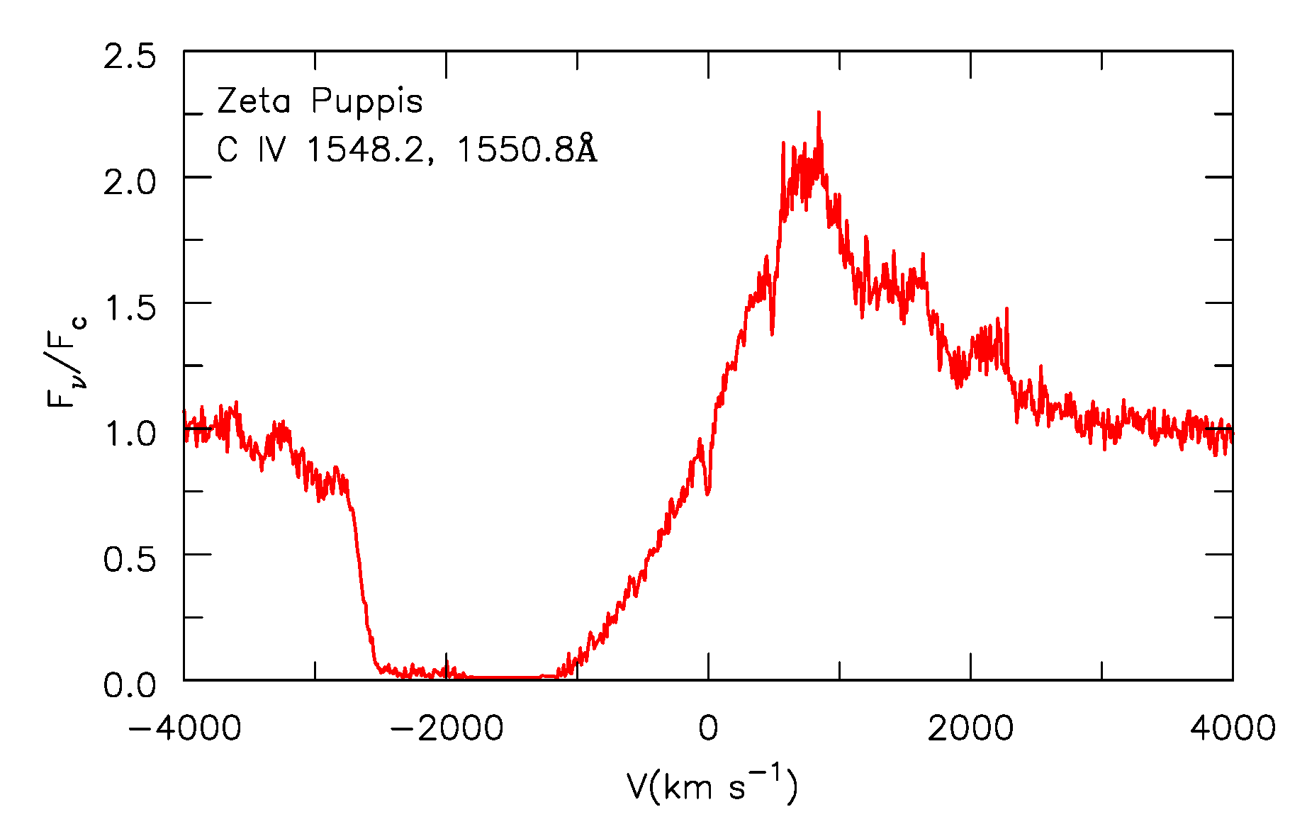
With the discovery of X-ray emission from O stars it was realized that X-rays could explain the presence of both O vi and N v P Cygni profiles7 in the UV spectra of O stars. An example P Cygni profile is shown in Figure 3. Since O stars typically have effective temperatures of K, the photospheric radiation field cannot produce sufficient O vi to explain the observed O vi profile. However, X-rays, through Auger ionization, can produce sufficient O vi [78]. In the case of O vi, the crucial reaction is:
O iv(1s2 2s2 2p) + X-ray → O v(1s 2s2 2p) + e− → O iv(1s2 2s) + 2e−.
Typically two electrons are ejected (i.e, one by interaction with the photon and one by the Auger process) in Auger ionization for CNO elements but for heavier elements more than two electrons can be ejected (e.g., [68]). In cmfgen we assume all inner-shell ionizations only eject two electrons and the intermediate states are omitted.8 Many studies have shown that inner shell ionization of X-rays can successfully explain the presence of O vi and N v in O stars (e.g., [79,80]). Auger ionization complicates the kinetic equations since more than two ionization stages are directly coupled.
4. Recombination
The recombination rate is given by
(e.g., [4]) where the subscript K refers to the recombining ion and the LTE population is computed using the actual electron density. The quantity (for a given level) is only a function of the electron density and temperature. When the gas is in LTE, and when , the photoionization and recombination rates (absolute values) are identical.
In my work I treat recombination as the reverse process of photoionization and hence in cmfgen recombination rates are computed using the photoionization cross-sections. As noted earlier, rates are evaluated using numerical quadrature, and identical weights are used for both the forward and reverse process. At high densities it is desirable to treat both processes identically since small differences can cause erroneous populations to be determined when solving the kinetic equations. At depth, where LTE conditions apply, it is important that they identically cancel. Generally the weights are evaluated using the trapezoidal rule—more accurate quadrature schemes are generally not feasible because of the complex frequency dependence (and depth dependence) of the radiation field, and because the same quadrature scheme must be used to compute the rates for both photoionization and recombination. Care must be taken near bound-free edges, since the integrand in the recombination rate can vary rapidly with frequency—especially true for highly ionized states at low temperatures since the recombination rate at frequency scales as .
For low densities, such as those found in H ii regions, planetary nebulae, and many collisionally ionized plasmas, recombination rates are often evaluated separately, and treated as a distinct process. At “low” densities most transitions are optically thin, and recombination into high states simply cascade into the ground state and metastable levels. In a H ii region, for example, the ionization of H is maintained through photoionizations from the ground state and photoionizations from excited states can be ignored. However transitions to the ground state can be optically thick. Consequently two limiting cases are considered when computing H line strengths—Case A, in which all transitions are assumed to be optically thin, and Case B, in which only the Lyman transitions are optically thick (e.g., [25]). Under the optically thick assumption the rate of decays in a transition is assumed to be exactly balanced by the rate of radiative excitations in the transition.
4.1. Direct Radiative Recombination
This process is taken to refer to simple recombination processes such as
In the above n and l refer to the principal and angular momentum quantum numbers of the electron.
H+ + e− → H(nl) + hν and
C iv(2s 2S) + e− → C iii(2s nl) + hν.
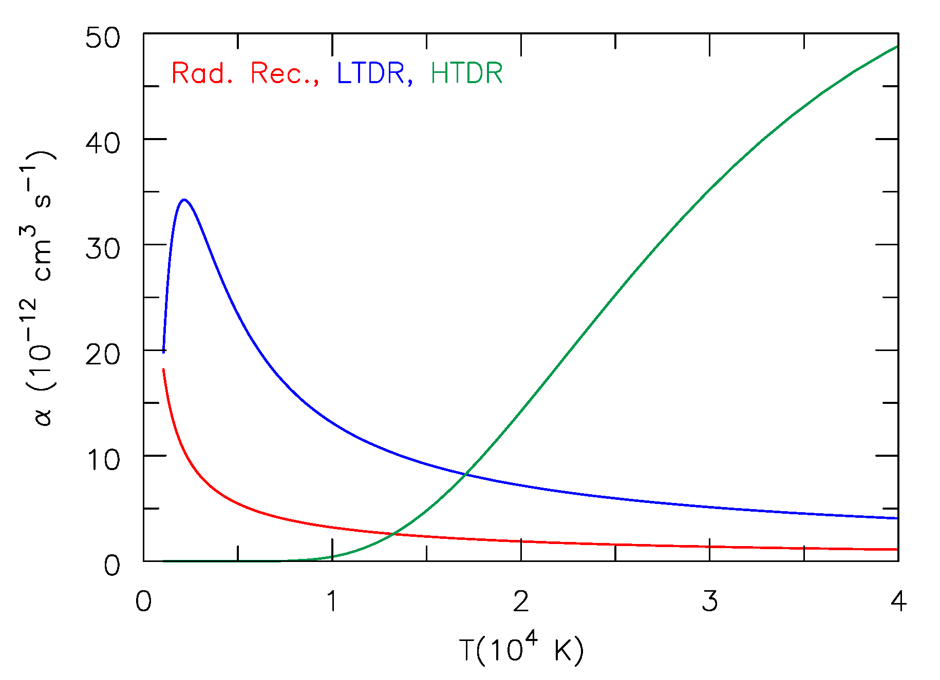
The cross-sections for the processes are “smooth” and easily integrated. However, state-of-the-art photoionization cross-sections, such as those available through TOPbase and NORAD, often include indirect photoionization routes or resonances. When discussing the reverse process it is often convenient to split the resonances into two classes—low temperature dielectronic recombination (LTDR) resonances and high temperature dielectronic recombination (HTDR) resonances.
4.2. Low Temperature Dielectronic Recombination (LTDR)
LTDR refers to recombination through double-excited states that lie close to, but above, the ionization energy of the ion ground state [81,82]. It is treated separately from HTDR since it is very species/ionization state specific—the energy levels involved in LTDR need to be known accurately since the distance of these states from the ionization limit is a crucial factor in determining the recombination rate. Dielectronic recombination is the inverse process of autoionization.
We can understand the LTDR process as follows by using an example. Consider the C iii 2p 4f D state (Figure 4) which can autoionize (the inverse process to dielectronic recombination) to give C iv and a free electron. For this state the autoionization rate coefficient is large (> s).9 However, the level can also undergo a “stabilizing transition”, leading to a recombination, with the most important stabilizing transition being
The Einstein A coefficient for this process () is (P. J. Storey, private communication), much lower than the autoionization probability. Consequently the 2p 4f F state will be in LTE with respect to C iv and hence the LTDR recombination rate for this single transition is where (in cgs units) is given by
(e.g., [4]). In the above formula is the statistical weight for the 2p 4d F state, is the statistical weight of the C iv ground state (2s S), is the electron density, is the ground state population of C iv, and is the energy of the 2p 4dF state above the ground state of C iv. At that single transition leads to a LTDR recombination coefficient (defined as the (LTDR rate)) of cm s (P. J. Storey, private communication) which is essentially identical to the direct recombination rate of cm s [83].
2p 4d 1Fo → 2p2 1D hν.
Thus, we see the following:
- The LTDR rate is very sensitive to when is of order unity or larger.
- When , the LTDR recombination rate scales as and thus increases more quickly with decreasing temperature than the radiative recombination rate, which typically scales as with . (see, e.g., [83]).
- The LTDR process will be most important for those states with a large Einstein A coefficient and for those states lying closest to, but above, the ion ground state.
- The process is very dependent on the details of the atomic structure. In the above case, the energy of the 2p 4d F state is crucial for determining the LTDR rate. As the LTDR autoionizing states lie well above the C iii ground state, and can have large energy widths, the energies of the states are not necessarily known. Theoretical calculations can provide estimates, but will have difficulties for states that lie ”very close” to the ionization limit since a small error in the energy level can make a big difference in the recombination rate, particularly at low temperatures.
The LTDR rate can exceed the direct recombination rate, and in many cases plays a crucial role in determining nLTE level populations, and observed line strengths (e.g., [81,82,84]).
The LTDR process is complicated by states that are forbidden to autoionize in LS coupling, such as the 2p 4d D state in C iii or the quartet states in C ii. In such cases the populations of these levels must be determined by solving the rate equations. These levels will be collisionally and radiatively coupled to states that can autoionize and, because of departures from LS coupling, they can also have non-zero autoionization rates which are larger than the radiative decay routes from the state. Thus, these levels can be an important additional recombination channel.
In cmfgen we handle the quartet states in C ii as part of our atomic models while the doublet autoionizing states are assumed to be in LTE with respect to the ground state of C iii and are not directly treated. Recombination through the quartet states is treated via the line transitions connecting them to lower levels, while transitions for the autoionizing states are treated via the photoionization cross-sections. Generally we assume the states within a term are populated according to their statistical weights, although this will not be valid for some levels since the autoionizing rates can depend strongly on their total angular momentum. For example, the autoionizing probabilities for the C ii 2s 2p(P) 4s P j = 1/2, 3/2, and 5/2 states are , , and <. These were obtained from the full width at half maximum tabulated by [84]. One issue, potentially important at high densities, is that we do not have accurate collisional cross-sections for the states not permitted to autoionize in LS coupling.
For C iii we typically assume, following [82], that all low lying states can autoionize. LTDR is easily taken into account via the photoionization cross-sections; however, the assumption is only necessarily valid for those states in which the autoionization rates (greatly) exceed other processes populating/depopulating the autoionizing state.
A potential problem in nLTE calculations is that, due to difficulties of current atomic codes to compute accurate energies, the resonances in the photoionization cross-sections are offset from their true positions. Such offsets are probably unimportant when computing the Rosseland mean opacity, but can be important for spectral studies. First, an inaccurate energy will influence the location of observable resonances in stellar spectra. Second, it can have an effect at “low” temperatures due to the scaling of the LTDR rate with temperature (). Third, complicated nLTE effects could arise. For example, a wrong resonance wavelength can potentially cause issues if a strong resonance coincides (or now does not coincide) with another bound–bound transition (since a strong resonance can affect the radiation field in the transition and vice versa).
The direct inclusion of resonances in photoionization cross-sections also has other potential issues. First, the resonances vary much more rapidly than the background cross-section and hence a very fine frequency grid needs to be used—this is particularly true for narrow resonances. For computational expedience, we typically sample the continuum cross-sections in cmfgen every 500 km s (but finer near level edges). To avoid aliasing10 we smooth the cross-sections. In early versions of the atomic data the cross-sections were smoothed to a resolution of 3000 km s but in new data sets we no longer store the smoothed cross-sections. Instead, newer cross-sections can be smoothed to the desired resolution, set by a control parameter, when they are read in.
Second, a narrow resonance can mean that the autoionization lifetime of the upper level may be comparable to, or even larger than, radiative transitions from the same level. As a consequence the upper level may not be in LTE with respect to the ion and hence the photoionization cross-section should not be used to compute the recombination rate. When identified, such a resonance should be clipped out and the upper levels treated as a bound state.
Third, photoionization cross-sections are usually computed in LS coupling. This means, for example, that the multiplet structure of the resonances is not treated—a problem more crucial when the resonances are “narrow”.
4.3. High Temperature Dielectronic Recombination (HTDR)
HTDR involves high Rydberg states [85,86] and it is very difficult to treat accurately in stellar atmosphere codes. The easiest way to visualize HTDR is to discuss a specific example.
Consider for example C iii whose ground state is 2sS where we have omitted the complete inner shell for simplicity. The states contributing to HTDR are the Rydberg states of the form 2p nl that converge on the C iv state 2p 2Po (Figure 4). Such states can autoionize to give C iv 2s S or the 2p electron can radiatively decay giving rise to C iii 2s nl. At “low” densities the nl electron will decay to a lower level, producing a “real” recombination. Since the autoionization rates decay slowly with n, and since the 2p → 2s transition probability is approximately constant, high n values (e.g., up to n = 100) determine the net recombination rates. Such levels are not typically included in nLTE calculations. The process is further complicated because the autoionizing rates strongly depend on the angular momentum—low “l” states have much higher autoionization probabilities than do higher angular-momentum states [85,87].
At low densities the HTDR recombination will scale roughly as where E is the energy of the 2s-2p transition in C iv. Since the energy of the 2s-2p transition is well known, and since the energy of the high Rydberg states is easily approximated, the accuracy of the energy levels is not a crucial factor determining HTDR rates. For some species, several Rydberg series may contribute to the HTDR rate, yielding a more complicated temperature dependence than the simple expression provided above.
5. Suppression of Dielectronic Recombination
5.1. Collisional Processes
The classic HTDR formula only applies at low densities. As the density rises, collisional ionization by electrons can significantly suppress HTDR. This has been explicitly considered for HTDR of C to C (i.e., C iv to C iii) by [88,89]. The authors of [89] found suppression factors of ∼0.7 at , at , at , and at cm (these data were read from Figure 1 in [90]). The reduction in the HTDR rate arises because the stabilizing transition (2p-2s in the case of C iii) from the autoionizing states leaves the electron in a high nl state. As the electrons cascade down to lower nl states, they can be collisionally ionized by electrons.
5.2. The Importance of the Radiation Field
The radiation field is typically regarded as unimportant in the dielectronic process, but in stellar atmospheres and winds, the process could effectively suppress recombination, as illustrated below. In principle, there are two suppression routes. The radiation field can directly suppress the stabilizing transition or the radiation field can directly ionize an electron out of the high nl state which the stabilizing transitions have left the ion in. The latter is similar to collisional suppression, except it is the radiation field, rather than collisions with electrons, which is reionizing the atom/ion.
For simplicity we treat the resonance as a line transition between two bound states, with the upper level being the autoionizing level. The net recombination rate will be given by
where is the mean intensity in the line and is given by
is the line absorption/emission profile (which, in general, is determined by the finite lifetimes of the levels involved in the transitions, thermal motions of the atoms, and the interaction of the radiating atom/ion with its neighbors (see [4], Chapter 9)) and is the line source function given by
In LTE and hence simplifies to the Planck function. As is readily apparent the net rate does not directly depend on the optical depth—such a dependence only occurs indirectly through the dependence of on the optical depth.
In nebula conditions is typically (since the nebula is very distant from the star the radiation field is greatly diluted) and the contribution to the recombination rate by this single transition is simply . When the rates are summed over all resonances you recover the LTDR/HDTR recombination rate. However, such a rate is typically an upper limit since the radiation field can reduce this rate.
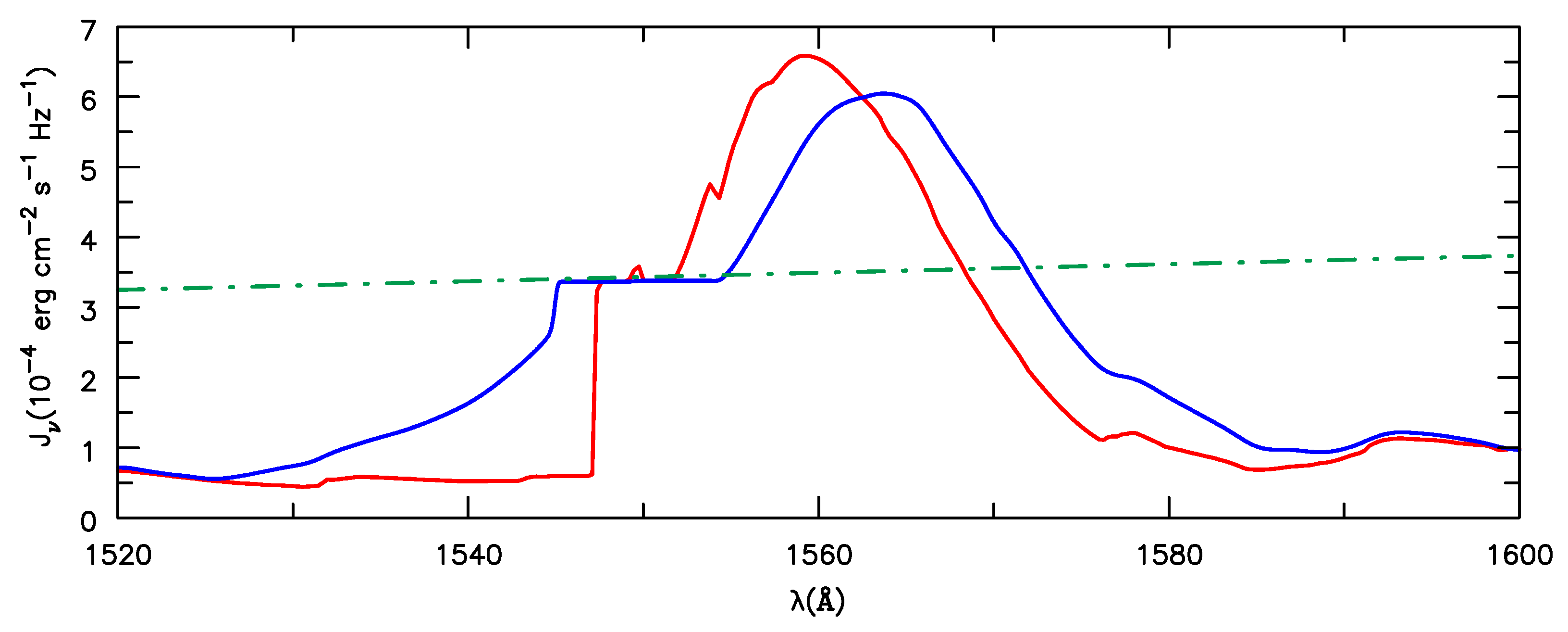
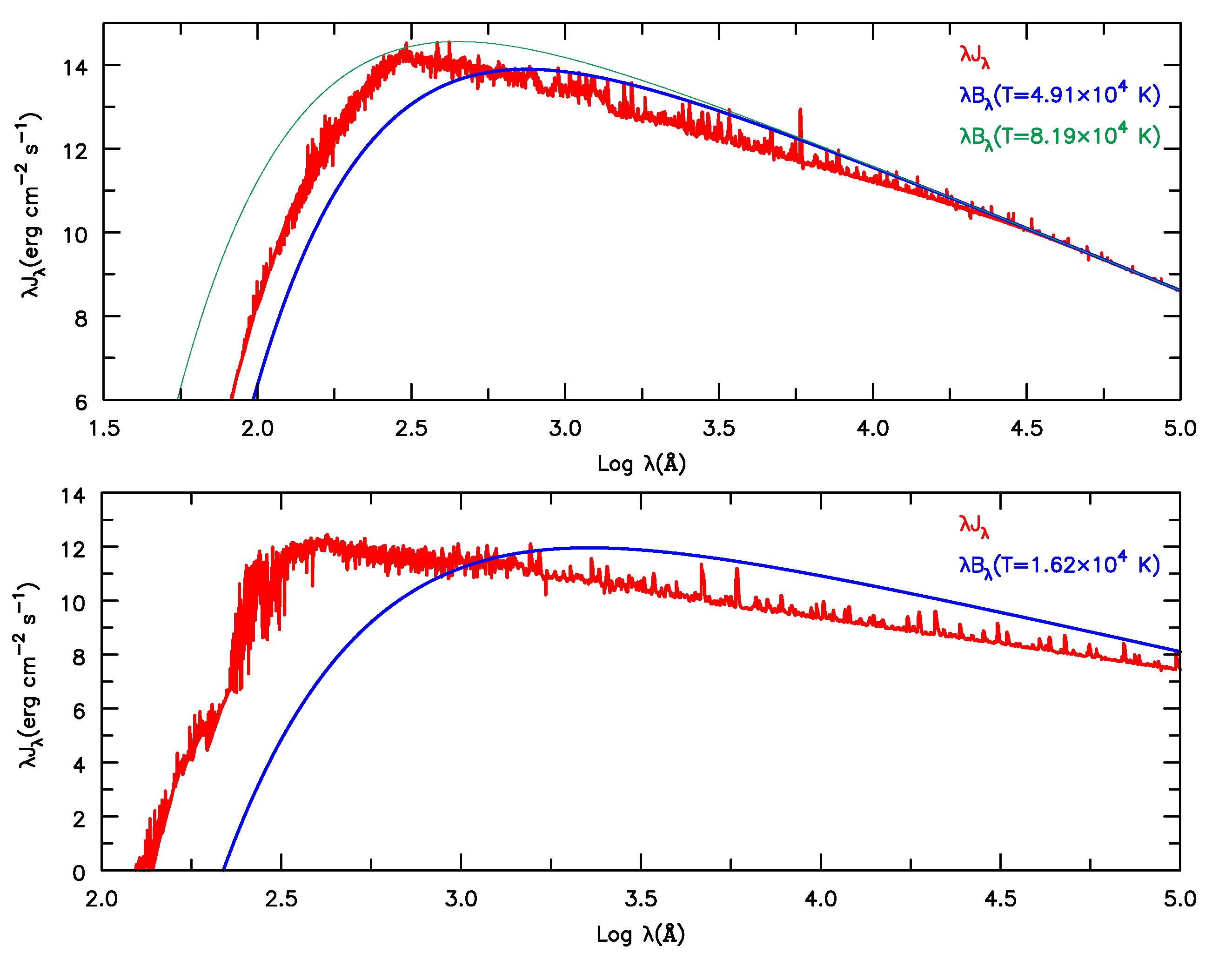
At depth in a stellar atmosphere , and thus the net LTDR and HTDR rates are identically zero—that is, every downward transition in the stabilizing transition is balanced by an upward transition. However, above the atmosphere the temperature of the radiation field and the electrons are not the same. Typically will fall below ; however, in a wind can be greater than in some transitions. In Figure 6 we show the mean intensity (in the comoving frame) and the blackbody mean intensity at a temperature of K and a density of electrons cm—roughly 50% of the emission in the line referred to as C iii originates above that density. From that figure we see that the radiation field at the wavelength of the C iv resonance transition, and at/near the stabilizing transition, is close to a blackbody at the local electron temperature. Thus, the radiation can act to suppress HTDR.
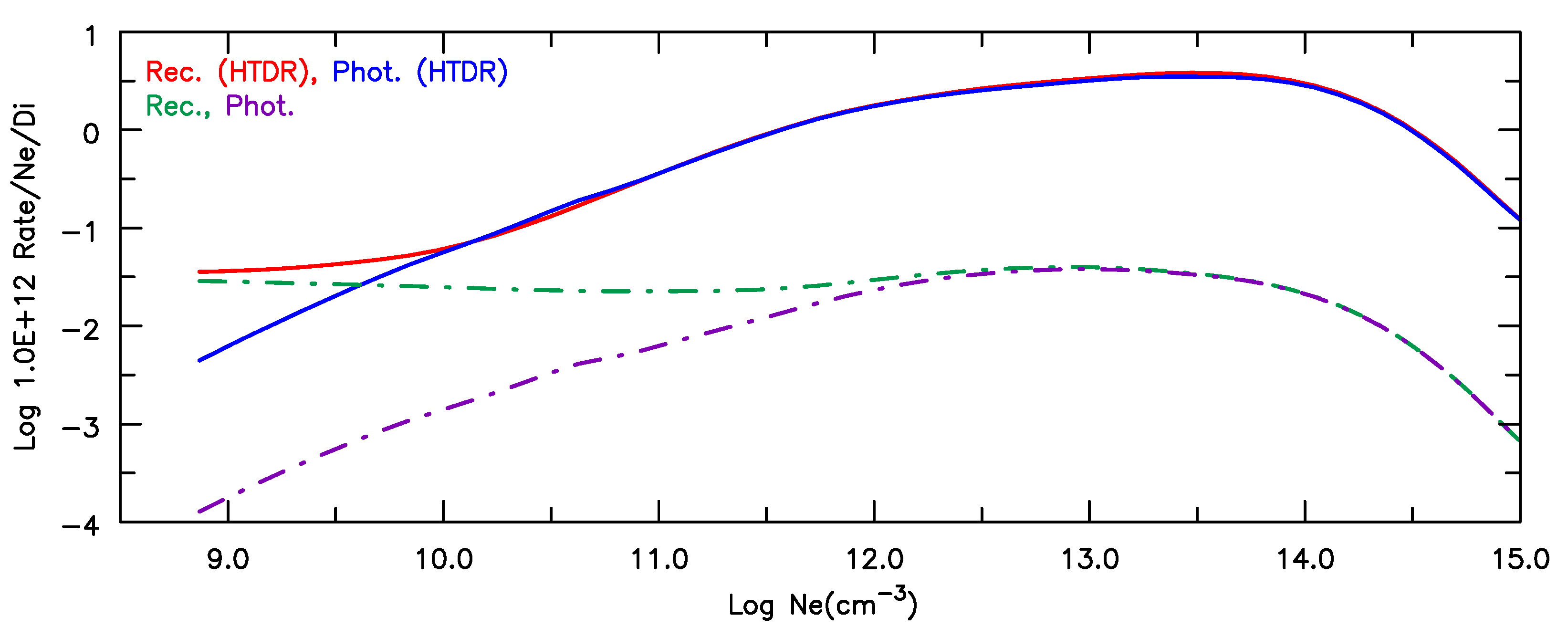
In Figure 7, we show the recombination and photoionization rates for through 30 singlet states of C iii (treated as a single level) for a test calculation in which we included HTDR transitions for levels up to , and with no suppression of the recombination rate with the angular orbital quantum number. The resulting model spectrum is almost identical to the spectrum computed without HTDR—a consequence of the low temperatures in the C iii line-formation region and the suppression of HTDR via the radiation field in the stabilizing transition. This result is model dependent—in practice the importance of HTDR needs to be examined on a case-by-case basis.
The influence of the radiation field is not an issue if the resonance is included as part of the photoionization cross-section as the influence of the radiation field is automatically taken into account. It is also not an issue for “autoionizing” states treated as bound levels, since the radiation field is again taken into account. However, it is a potential issue if the LTDR or HTDR rate is included as a separate process, and the inverse process is not included.
6. Astrophysical Examples
Below we discuss some examples of where photoionization data is crucial. It is unrealistic to discuss all cases, since photoionization data is crucial in any photoionized plasma and is crucial for nLTE analyses. For some plasmas, in which collisional processes dominate, photoionization is less important but the inverse process (recombination) is still critical.
6.1. Recombination Processes
The importance of photoionization/recombination processes depends critically on the application. Here we discuss photoionized plasmas and gradually work our way up in density.
In ionized nebulae and H ii regions H and He lines are produced by recombination, while the ionization is typically maintained via ionizations from the ground state. The strongest metal lines (i.e., those not due to H and He), such as O iii and N ii, typically arise via collisional excitation from the ground state. Metal recombination lines are much weaker, simply because the metal abundances are typically a factor of (or more) lower than that of H. Some other lines are produced by line fluorescence, where the radiation field in a bound–bound transition in one species gives rise to line emission in another species (the Bowen mechanism). For example, some O iii lines in planetary nebulae (gaseous nebulae surrounding stars with effective temperatures in excess of 30,000 K) are produced by the chance overlap of an O iii line with He ii Ly [25,92]. With high signal-to-noise spectra metal recombination lines are seen (e.g., [93,94]) and for most lines their strength is effectively set by optically thin recombination (radiative and dielectronic) theory.
As the density increases, processes become increasingly complex. More transitions become optically thick, affecting the cascade process and hence line strengths. Collisional coupling between the levels also becomes more important. If the radiation field is not too diluted, photoionization from excited states also becomes increasingly important. For example, in O and WR stars, the ionization of He to He occurs predominantly from the state whose population is maintained via the intense radiation field in Ly [95]. Similarly, the ionization of C iv is maintained from the levels.
As the density further increases, lines become thicker and photoionization/recombination can become more important since continuous processes at many wavelengths remain optically thin. In hot stars the departure coefficients (=) for H and He ii levels typically rise above the photosphere. Bound–bound transitions are optically thick, preventing cascades. The radiation is diluted, hence recombinations into a level typically exceed photoionizations from that level. Eventually, however, photon escape in lines becomes important and the departure coefficients decrease. However, one must be careful with generalizations—at some wavelengths (particularly in the Wien regime of the blackbody curve) the rapid fall of the electron temperature with height above the photosphere means that the energy density in the radiation field may initially exceed the radiation energy density predicted by the blackbody formula for the local electron temperature.
Bound–bound processes are crucial for determining line strengths. However, it is ultimately photoionization and recombination that determines the ionization state. In some cases, charge exchange processes are crucial [96,97]. Particularly important are charge exchange process of neutral H with, for example, Fe and O. The reaction
is resonant, has a total rate coefficient of order cm s [98], and is crucial for determining the O/O ratio in regions where the neutral hydrogen fraction exceeds roughly .
6.2. The Sun
For the Sun, our nearest star, we can determine its structure in two ways. First, we can use the observed Solar parameters (M, L, , abundances) to construct a theoretical model of the Sun. Second, we can use helioseismology observations to constrain the internal structure11. Unfortunately, the structure determined from theoretical models and that determined from the helioseismology observations are inconsistent. They can be reconciled if the adopted opacities (for the relevant temperatures) are too low. This could arise if the adopted O abundance is too low or alternatively it could arise from inaccuracies in the opacities (i.e., inaccuracies in the photoionization cross-sections, oscillator strengths, etc). The resolution of the problem is still unclear [50,99,100].
6.3. O, WR, and LBV Stars
O stars are the most luminous hydrogen-core burning stars known. They have masses in the range 30 to ∼100 and luminosities typically greater than . Due to nuclear processing H is being converted to He in the core. At the same time most of the C and O initially present have been converted to N. Mass loss, and mixing, then operate to reveal this nuclear process at the stellar surface. During later evolution stages He is converted to C and O, and mass loss can also reveal this material at the stellar surface.
All massive stars are losing mass in a stellar wind. In O stars and their descendants (e.g., LBVs, WR stars) the winds are driven by radiation pressure. Due to their high luminosities the stars are close to the Eddington limit12. Consequently, it is relatively easy for radiation pressure acting through bound–bound transitions to drive material off the surface of the star via a stellar wind. Due to instabilities in the line driving, it is believed that the winds are highly clumped (e.g., [73,74,75]). Additional evidence for clumping comes from variability studies (e.g., [101,102]), from the anomalously low strength of some UV resonance transitions relative to the level of H emission (e.g., [33,34,35]), and the weakness of electron scattering wings associated with strong emission lines in P Cygni stars and WR stars13 [103,104].
The wind density in massive stars varies considerably. For main sequence O stars the winds are relatively weak and only affect a few spectral features. Their photosphere is geometrically thin (i.e., radius of the star) and, in principle, can be modeled using plane-parallel model atmospheres (i.e., the curvature of the star’s atmosphere can be ignored), although the wind may still have an influence at some wavelengths. As the stars evolve, the wind density tends to arise and become increasingly important, and the use of a plane-parallel atmosphere is no longer valid. Indeed, in WR stars, the wind is so dense that spectrum formation occurs in the stellar wind and nLTE spherical models that treat the wind are essential.
6.3.1. N iii and N iv lines in Of and WN stars
Of stars are evolved O stars that show emission in N iii and He ii [105,106]. First computations of model atmospheres suggested that the N iii lines are driven into emission by LTDR [107]. However, more recent work that includes line blanketing (by lines of iron group elements) and winds reduces the importance of dielectronic recombination, and continuum fluorescence acting through UV resonance transitions plays a crucial role [108].14
WN stars, which are a type of WR star, are evolved O stars which show abundances which have been influenced by the CNO nuclear burning cycle—H is depleted (in many it is absent), He is enhanced, and much of the C and O has been converted to N. In a WN star such as HD 50896, several N iv lines are seen. The formation of these lines is complex, but typically their strength is determined by a combination of dielectronic recombination and continuum fluorescence [110]; while the models used by [110] did not include iron group elements, more recent models with iron-group elements confirm the importance of LTDR for WN stars. In Figure 8, we illustrate the influence of LTDR on several N iv emission lines for a model appropriate to an early-type WN star (such as HD 50896).
6.3.2. Carbon in WC stars
WC stars are the evolved descendants of WN stars. Due to extensive mass loss, and nuclear processing in the interior of the star, their atmospheres are devoid of H, and are primarily composed of He, C and O (with similar mass fractions). Due to their dense stellar winds, and high C and O abundance, emission lines of He, C, and O dominate the spectrum. In the optical region, most of these arise from recombination, although optical depth effects greatly complicate line formation [91].
Below we discuss the spectrum of the WC4-type star, BAT99-9, which has recently been discussed by [37]. In most ways its spectrum, and parameters, are typical of other WC4 stars in the Large Magellanic Cloud (LMC). However, it does differ in one important aspect—it still exhibits one N v and two N iv emission lines. Nitrogen is expected to disappear rapidly as a star transitions from WN to WC because N in the interior of the star is converted to Ne.
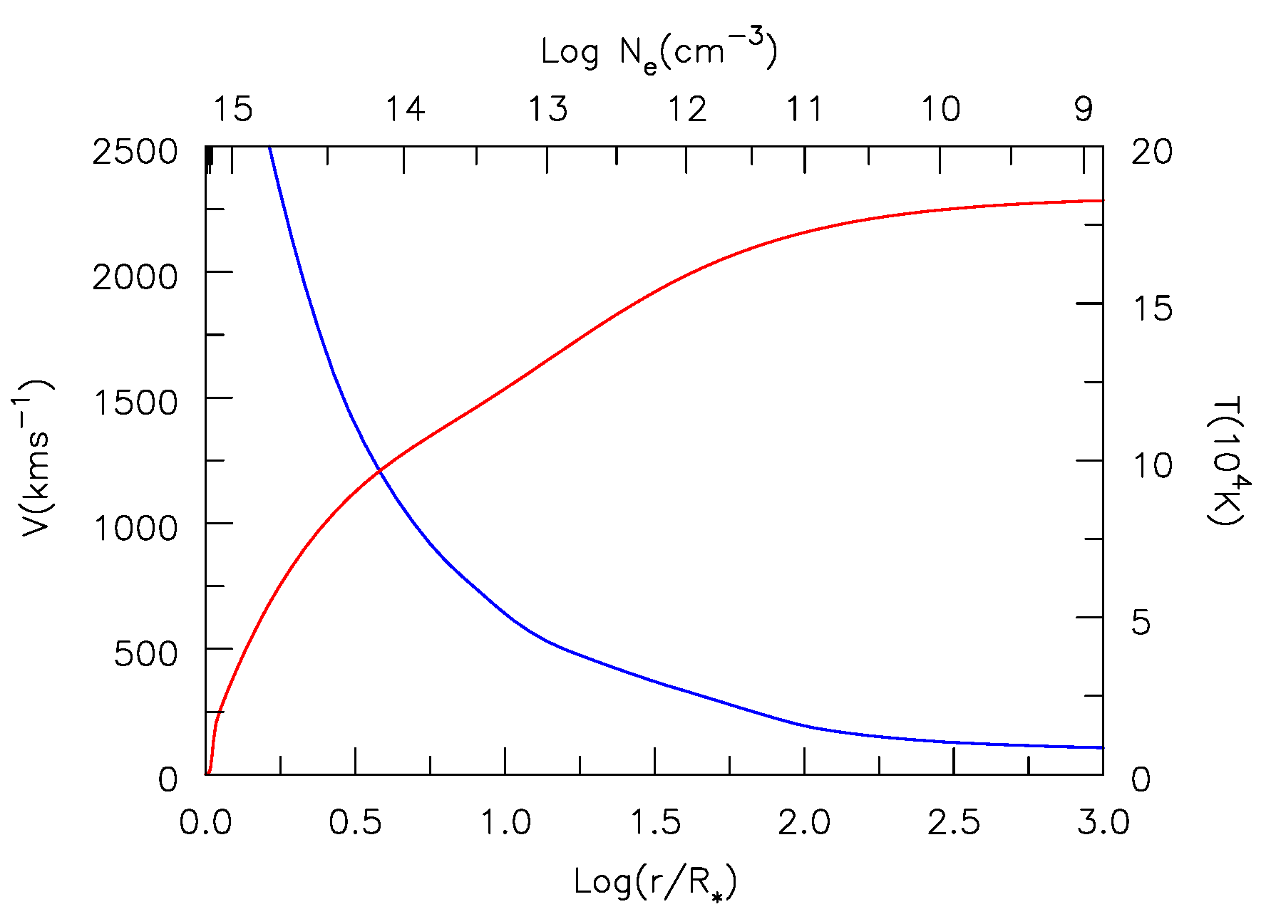
The electron temperature structure and wind velocity of a model for the LMC WC4 star, BAT99-9, is shown in Figure 9. The non-Planckian nature of the radiation field at two depths in the wind is illustrated in Figure 10.
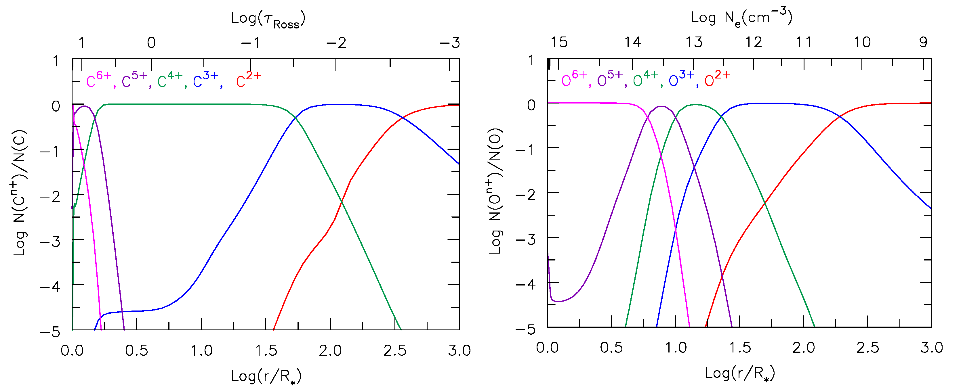
A characteristic of WC stars is the stratified ionization structure—as we move farther out in the wind the ionization decreases. The complex ionization structure for C and O is illustrated in Figure 11. Because of stratified ionization structure many different species need to be included to model the spectrum. In BAT99-9 we see emission from four stages of O (O iii through O vi). To understand driving at the base of the wind additional ionization stages are needed—in some models we include Fe iv through Fe xvii.
The stratified ionization structure is a consequence of several factors. First, the winds of WR stars are not transparent. For example, the He ii Lyman continuum (shortward of 228 Å) is optically thick. Further, the transparency is a strong function of wavelength. Second, as we move out in the wind the radiation field becomes diluted. Third, the intense radiation field in some spectra bands can pump low lying levels. Because of this, and because of the high densities which reduce cascades, ionizations from excited states can play an important role in determining the ionization state of the gas.
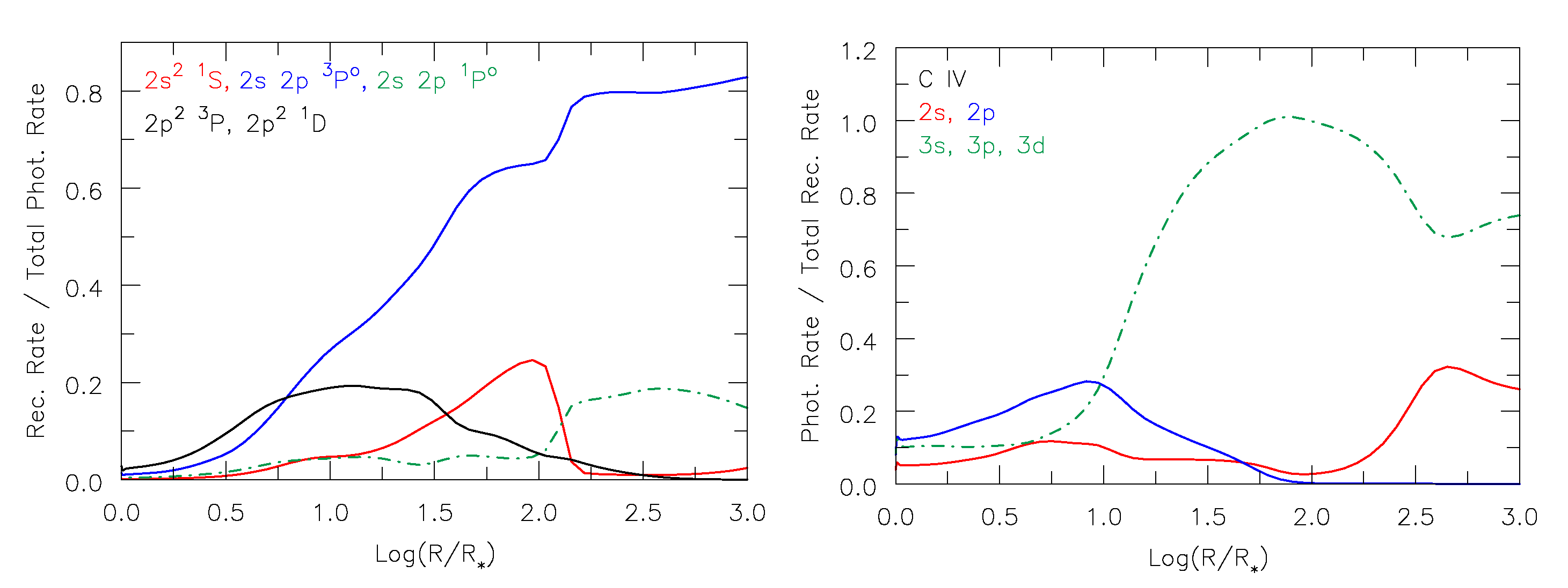
In Figure 12 we illustrate the photoionization rate, normalized by the total recombination rate to all (included) levels. The normalization was primarily chosen to emphasize the important process in the line formation region. In the inner regions of these dense winds photoionizations and recombinations to each level will be in detailed balance. As we move out in the wind the photoionization from most levels will decrease due to dilution of the radiation, although for some levels the photoionization and recombination rates may maintain equality if the continua are optically thick. For C iii we see that three levels, in order of importance, control the ionization—2s 2p P, 2s S, and 2s 2p P. On the other hand, for C iv it is the n = 3 levels (3s, 3p, and 3d) that help to determine the C iv/C v ionization ration. The ionization eventually shifts because the radiation is becoming diluted (as ) and the populations of the n levels are also declining. One reason for the difference in behavior of C iii and C iv is there is often a rapid decline in the strength of the radiation field shortward of ∼228 Å.
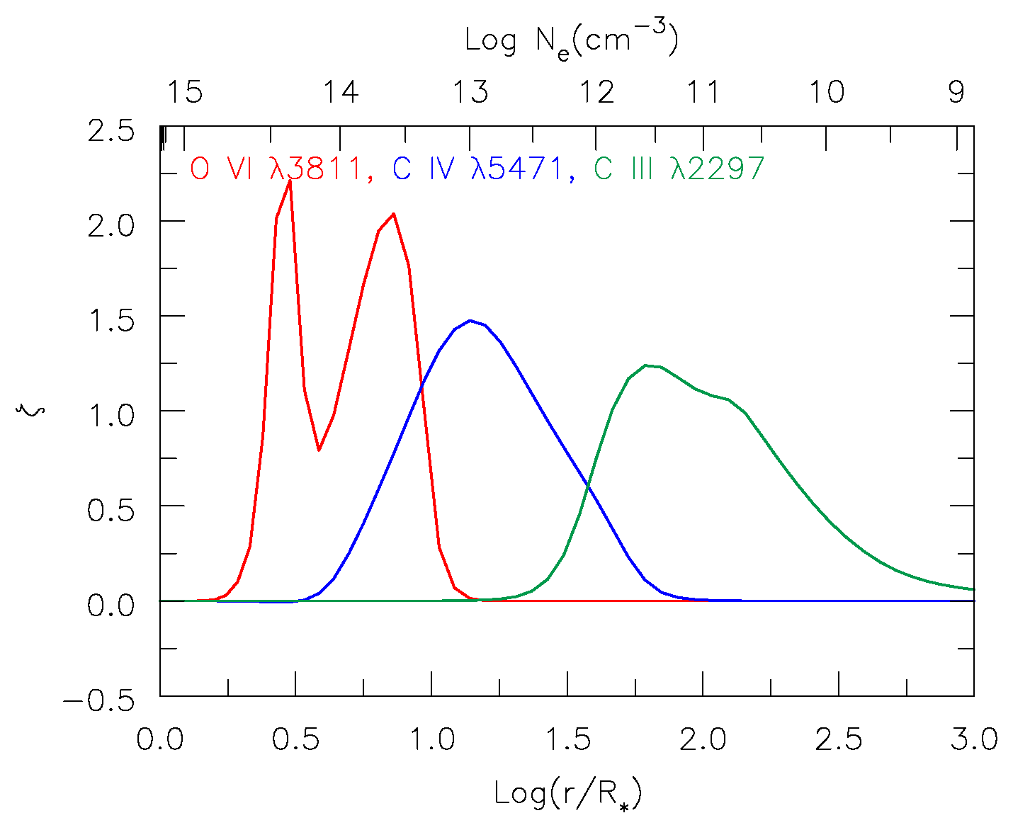
The presence of multiple ionization stages in the wind results in emission from multiple ionization stages. For example, in the case of BAT99-9 we see emission from two ionization stages of carbon (C iii & C iv)15 and four ionization stages of oxygen (O iii through O vi) with the characteristic line width (after allowance for blending and for the formation mechanism) decreasing as the ionization increases. The origin of one O and two C lines is shown in Figure 13—it shows that a given emission line originates over a range of radii and that lower ionization features form farther out in the wind.
6.4. C ii in [WC] Stars
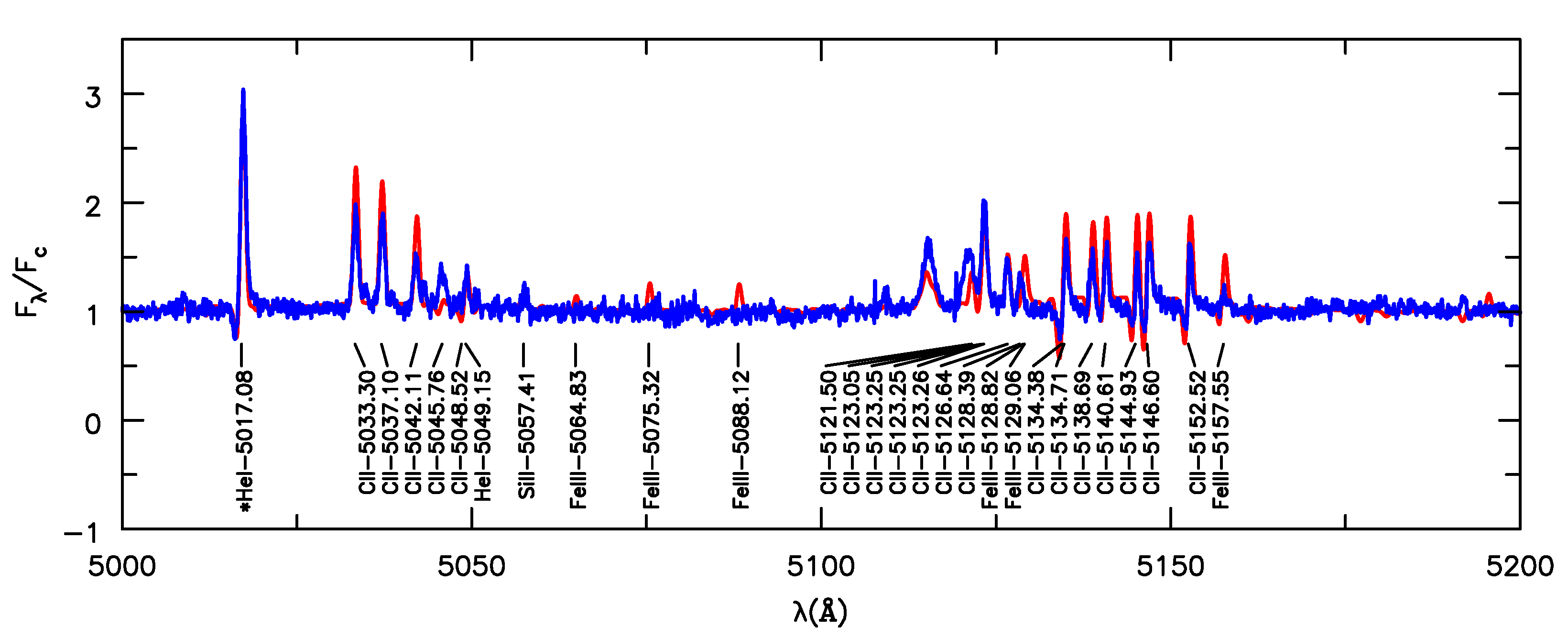
The LMC star J060819.93-715737.4 (hereafter J0608) has an exquisite C ii spectrum—over 150 lines can be identified in the optical [112,113]. It is classified as a [WC11] star with the [] denoting that it is associated with a low mass star () rather than the product of the evolution of a massive star.16 The star is probably devoid of H (the observed spectrum exhibits H emission but these probably arise in circumstellar material and not in the stellar wind) and the C abundance is substantially enhanced (atmospheric mass fractions of He and C are approximately 0.4 and 0.6, respectively); while the rich C ii spectrum is predominately produced by recombination, it cannot be explained by classical optically thin cascades—optical depth effects play a crucial role in determining the relative C ii line strengths.
The spectrum of J0608 is similar to the [WC11] star CPD–56 8032 whose spectrum has been extensively discussed and analyzed [114,115,116,117]. Those studies show the importance of LTDR in producing the spectrum and identify several optical lines that arise from autoionizing levels. The spectrum of J0608 has slightly lower ionization than CPD–56 8032 and has a lower terminal wind speed, and as a consequence provides a more ideal object by which to explore the C ii spectrum.
A small section of the rich C ii spectrum is shown in Figure 14. The authors of [113] argue that some of the lines are formed via fluorescence processes, but our own modeling suggests that the spectrum can be explained by allowing for the optical depth effects and by allowing for a transition from ionized to neutral carbon in the outer wind. The latter truncates the emission of the strongest C iii lines.
In Figure 14, we also show a free–free resonance (∼ 5115 Å) previously identified in CPD–56 8032 [117]. The observations were obtained with a resolution of 7 km s and hence the line is resolved. In cmfgen the resonance is treated as a free–free resonance since both levels involved in the transition are autoionizing (with A∼; [117]). In the case of this free–free resonance it was trivial to omit it from a “continuum” calculation. The latter is needed so we can rectify the spectrum (i.e., normalize the continuum to unity). However, this is not the case for bound-free resonances that appear in the photoionization cross-sections. Such resonances can appear in the computed continuum, distorting an otherwise smooth spectrum. These resonances riddle the UV continuum spectrum. However, in practice they are difficult to discern because of the rich forest of bound–bound transitions which mask the continuum spectrum.
6.5. Supernovae
Supernovae are fascinating objects. They represent the end points of evolution for many stars and are an important source of metals (astronomical jargon for all elements more massive than He) in the Universe. Broadly speaking there are two classes of supernovae —those arising from the core collapse of a massive star (e.g., [120]) and those arising from the thermonuclear detonation of a white dwarf (WD) star (a compact object of stellar origin with a mass less than that is supported by electron-degeneracy pressure). The latter class is designated as a Type Ia SN and, while we know that it involves a WD, we do not know in what type of binary system the explosion occurs.
An extensive discussion of the possible progenitors of Type Ia SNe is given by [121]. Type Ia SN could arise when the WD accretes hydrogen-rich material from a “normal” star (e.g., a red supergiant or a main sequence star). As a WD accretes mass its radius shrinks (assuming it does not eject the accreted mass via a surface explosion in an event called a nova, which is believed to occur in many systems). As it approaches the Chandrasekhar mass of 1.414 (the upper mass limit or a WD star) it will undergo a thermonuclear explosion. Another possibility is that the WD star accretes He rich material from a WD companion. This material undergoes a surface thermonuclear explosion which triggers an inward propagating shock that triggers the detonation of the accreting WD. A third possibility involves collisions and mergers of two WD stars. In the first scenario the exploding WD has a mass of , while in the other two cases the mass of the exploding WD is (typically) less than . The different scenarios predict different chemical compositions for the ejecta and thus determining the chemical composition of the ejecta offers a potential means of determining the nature of exploding WD.
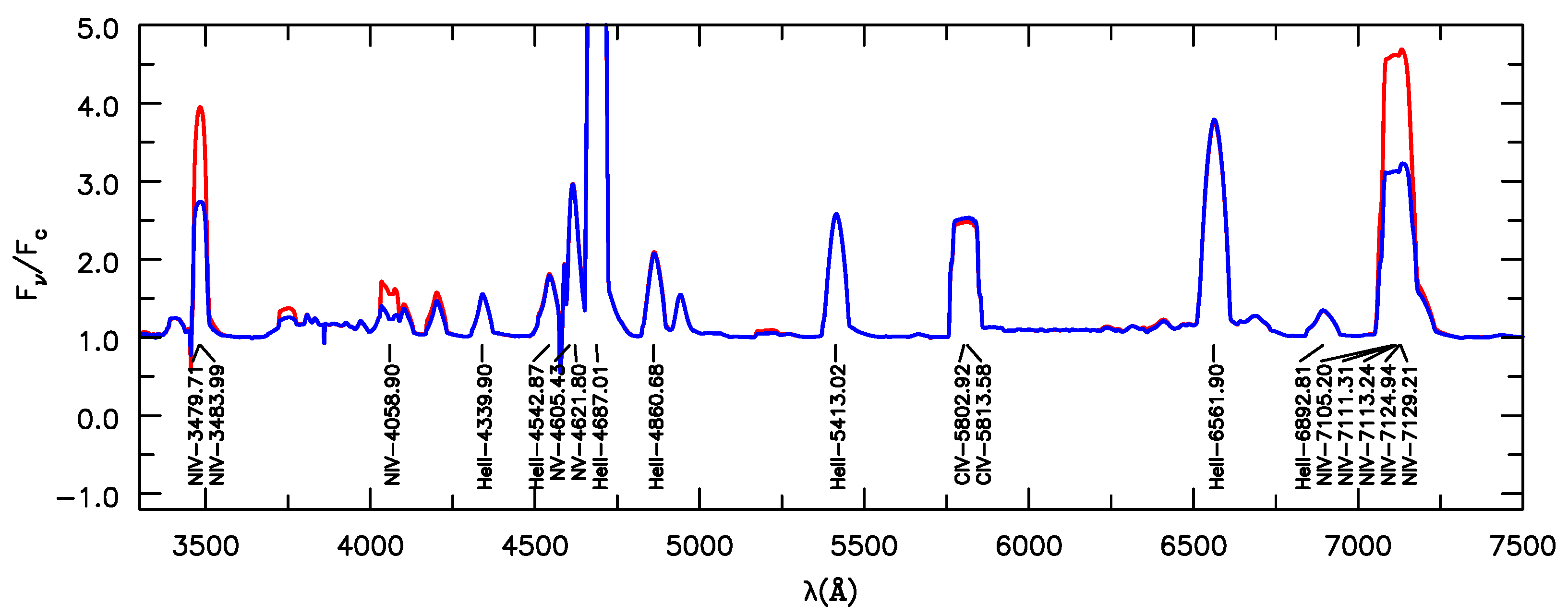
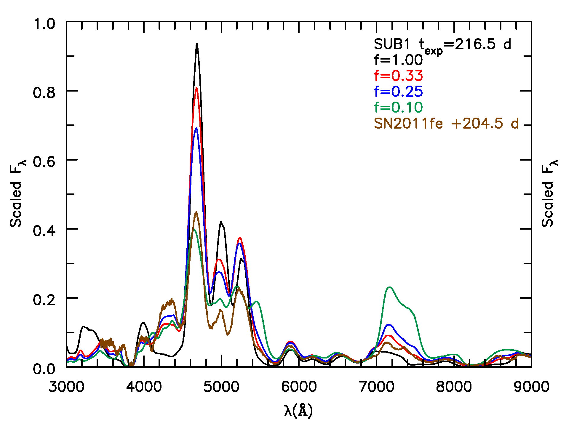
At late times (say 200 days) the spectra of Type Ia supernovae ejecta are dominated by emission lines of Fe, although lines due to Ni, Ca, and S are also present. One issue with current models of the ejecta is that they fail to yield an iron spectrum in agreement with observation (e.g., [45,122]). Basically, the Fe ii lines are too weak relative to Fe iii (Figure 15) and this limits our ability to interpret ejecta observations. Is the issue related to a problem in the ejecta explosion models, is it due to the ejecta being clumped (which enhances recombination and hence lowers the ionization), is it due to issues with the iron atomic data, is it due to problems treating the thermalization of high-energy electrons [122], or are we missing additional physics? Unfortunately in these systems the iron atomic data is of crucial importance, since Fe ii/ Fe iii is of order unity and the lines of both species probably form in the same region. Thus, a factor of 2 error in the Fe ii recombination rate will make a factor of 2 error in the Fe ii/ Fe iii ionization fraction and will change the relative line strengths (which are produced via collisional excitations) by a factor of 2. Fortunately, for Fe ii and Fe iii, HTDR is unimportant at the relevant temperatures, as can be gleaned from the rates provided by [123].
7. Conclusions
Accurate photoionization cross-sections are essential for many areas of astrophysics. The required quality varies greatly with the application. The biggest needs are at “intermediate” densities where nLTE is relevant, and where complex density and radiation processes directly affect level populations. This is the case for many astrophysical phenomena associated with, for example, stellar winds, accretion disks, and supernovae ejecta.
Funding
Partial support for the work was provided by NASA theory grant 80NSSC20K0524 and STScI Grant No HST-AR-16131.001-A. STScI is operated by the Association of Universities for Research in Astronomy, Inc., under NASA contract NAS 5-26555.
Data Availability Statement
cmfgen, and the atomic data used by cmfgen, are available at www.pitt.edu/hillier (accessed on 1 February 2023). This site also contains some older O star models. Data from supernova calculations can be downloaded from Zenodo or requested from the appropriate author. A grid of spectra are available from the Pollux data base [124]. A large grid of cmfgen spectra models has been constructed and is being made available [125,126]. Hillier will also provide cmfgen models upon request.
Acknowledgments
The author would like to thank P. J. Storey for extensive discussions on atomic data, and for supplying atomic data on C ii and C iii that was directly used in this review. He would also like to thank the numerous workers who have undertaken extensive atomic data calculations and made their work freely available on the internet. A special thanks to Nidia Morrell who obtained the high resolution spectrum of J0608. The invaluable comments made by the referees are also greatly appreciated. This paper has made use of NASA’s Astrophysics Data System Bibliographic Services.
Conflicts of Interest
The authors declare no conflict of interest.
Abbreviations
The following abbreviations are used in this manuscript:
| ADS | Astrophysics Data System |
| ESA | European Space Agency |
| HST | Hubble Space Telescope |
| LTE | Local thermodynamic equilibrium |
| nLTE | Non-local thermodynamic equilibrium |
| LTDR | Low temperature dielectronic recombination |
| HTDR | High temperature dielectronic recombination |
| LBV | Luminous blue variable |
| LS coupling | Total orbital angular momentum (L) is coupled with the total spin (S) |
| NASA | National Aeronautics and Space Administration |
| SN | Supernova |
| WD | White dwarf |
| WR star | Wolf–Rayet star |
| WN | Wolf–Rayet star belonging to the nitrogen sequence |
| WC | Wolf–Rayet star belonging to the carbon sequence |
| 1 | The effective temperature of the star is defined by the relation where L is the stellar luminosity (energy emitted per second), the Stefan–Boltzmann constant, and is the radius of the star. |
| 2 | The meaning of “accurate” is highly context dependent. Atomic data calculations can, in some cases, give energy levels accurate to 1% and for some purposes this is sufficient. However, for spectral modeling such energy levels cannot be used to compute transition wavelengths—a 1% shift (which will be potentially larger if the levels are close in energy) will move a line far from its correct location, influencing spectral synthesis calculations. Moreover, in non-LTE a wrong wavelength will influence how a line interacts with neighboring transitions. In O supergiants two weak Fe iv lines, that overlap with He i 304, influence the strength of He i singlet transitions in the optical and accurate wavelengths (and oscillator strengths) of these Fe iv lines are crucial for understanding the He i singlet transitions [1]. |
| 3 | Strictly speaking, a radiation temperature is only well defined if the radiation field is Planckian. However, astronomers often use color temperatures, defined by fitting a scaled blackbody ratio to the flux at two wavelengths, to characterize the nature of the radiation field in some pass band. In nLTE, astronomers may also use the excitation temperature to characterize the excitation or ionization state of a gas. In general these will not be the same as the local electron temperature, and will vary with level and ionization stage (though possibly in a systematic way). |
| 4 | The Sun’s atmosphere is cool and dense enough for molecules to form and 50 molecular species have been identified [8]. In the solar spectrum, spectral features due, for example, to CO, SiO, H, OH, CH, C, and CN, have been identified [8,9]. Dust formation in red giants and supergiants is common but not well understood [10], and in some cases may be associated with non-equilibrium chemistry [11]. |
| 5 | Throughout the article we neglect full shells when providing the electron configuration. We use the principal quantum number (n), orbital angular momentum number ( s, p, d, f, g …), and spin () to describe the state of an electron. Thus, 2p indicates an electron with and . LS-coupling (in which the orbital angular momenta are coupled and the electron spins are coupled) is used to provide the term designation. A term designation has the format 2S+1Lx where S is the sum of the (valence) electron spins, L is the total orbital angular momentum, and “o” is used to indicate that the arithmetic sum of the electron orbital angular momenta is odd (o) or even (in which case e is omitted by convention). An excellent primer on atomic spectroscopy is provided by [63]. |
| 6 | WR stars are a class of massive stars that evolved from O stars (stars with initial masses ≳ 15 ). They are experiencing mass loss via a stellar wind (induced by radiation pressure acting through bound–bound transitions) with a mass-loss rate typically in excess of and a terminal wind speed of ∼1000 to 3500 km s [64,65]. In many WR stars the wind is sufficiently dense that the entire spectrum we observe originates in the wind—the hydrostatic core of the star is not seen. There are two main WR classes: WN stars exhibit N and He (and sometimes H) emission lines, and exhibit enhanced N and He at the stellar surface due to the CNO cycle (the main H-fusion chain in massive stars). WC stars exhibit emission lines of He, C, and O, with a C abundance comparable to that of He (e.g., [66,67]). They have lost all of their hydrogen envelope, with the enhanced C abundance arising from the triple alpha process (3 HeC). |
| 7 | A P Cygni profile is formed when continuum radiation is absorbed and scattered by outflowing material. Outflowing gas along the line of sight absorbs continuum radiation and scatters it out of the line of sight, producing blue-shifted absorption. Radiation absorbed in other directions can be scattered into the line of sight and, for a spherically symmetric expanding gas, the combination with the blue-shifted absorption will give rise to red-shifted emission. |
| 8 | The ejecta of Type Ia SNe are composed primarily of intermediate mass elements (Ca, Si) and iron group (Fe, Ni, Co) elements. In such ejecta we may need to treat Auger ionization more rigorously since it could potentially affect the ionization state of the gas and the thermalization of non-thermal electrons. The non-thermal electrons are initially produced via Compton scattering of gamma-ray photons produced from decay of radioactive Ni and Co. In this case inner shell ionization will most likely occur via non-thermal electrons. However the subsequent Auger ionization and fluorescence are independent of how the K-shell hole was created. |
| 9 | From autostructure calculations made by a collaboration of researchers at Auburn University, Rollins College, the University of Strathclyde, and other universities. Tables produced by N. R. Badnell and are available at Atomic Data from AUTOSTRUCTURE. |
| 10 | A signal processing term that refers to the distortion of data due to sampling which is too coarse. In the present case a narrow but strong resonance could be missed in the photoionization cross-section when the frequency sampling is too coarse. Alternatively, its influence could be artificially enhanced if it is not fully resolved. |
| 11 | The Sun is simultaneously oscillating in thousands of different vibration modes. The frequency and strength of these modes depends on the internal structure of the Sun (e.g., the depth of the convection, the sound speed). |
| 12 | At the Eddington limit the force arising from the scattering of radiation by free electrons matches the gravitational force. |
| 13 | The strength of most emission lines in WR stars is proportional to the density squared. Thus, a clumped wind can yield the same line strengths for a lower mass-loss rate (i.e., for a lower average density). On the other hand electron scattering line wings arise from Thomson scattering of line photons by free electrons and hence scale with density. Thus, the strength of electron scattering wings relative to their neighboring emission line can act as a global diagnostic of clumping. In WR stars the wings are offset to the red from their originating transition because of the large outflow velocities. |
| 14 | In this process a strong transition (typically in the UV) absorbs continuum photons, a process whose efficiency is enhanced by the velocity field which allows the UV transitions to intercept more continuum radiation. In many cases the absorbed photons will typically be re-emitted in the same transition. However, in some cases the upper levels have an alternate decay route—decay via this transition can then lead to emission in this bound–bound transition. This is also known as the Swings mechanism [109]. |
| 15 | C ii emission is also predicted but this is masked by blending with other lines. |
| 16 | The 11 appended to WC denotes the ionization class of the star—in this case, a spectrum dominated by C ii with little evidence for C iii. |
References
- Najarro, F.; Hillier, D.J.; Puls, J.; Lanz, T.; Martins, F. On the sensitivity of He I singlet lines to the Fe IV model atom in O stars. Astron. Astrophys. 2006, 456, 659–664. [Google Scholar] [CrossRef] [Green Version]
- Nave, G.; Johansson, S. The Spectrum of Fe II. Astrophys. J. 2013, 204, 1. [Google Scholar] [CrossRef] [Green Version]
- Clear, C.P.; Pickering, J.C.; Nave, G.; Uylings, P.; Raassen, T. Wavelengths and Energy Levels of Singly Ionized Nickel (Ni II) Measured Using Fourier Transform Spectroscopy. Astrophys. J. 2022, 261, 35. [Google Scholar] [CrossRef]
- Mihalas, D. Stellar Atmospheres, 2nd ed.; W. H. Freeman and Company: San Francisco, CA, USA, 1978. [Google Scholar]
- O’Dell, C.R.; McCullough, P.R.; Meixner, M. Unraveling the Helix Nebula: Its Structure and Knots. Astrophys. J. 2004, 128, 2339–2356. [Google Scholar] [CrossRef]
- Benedict, G.F.; McArthur, B.E.; Napiwotzki, R.; Harrison, T.E.; Harris, H.C.; Nelan, E.; Bond, H.E.; Patterson, R.J.; Ciardullo, R. Astrometry with the Hubble Space Telescope: Trigonometric Parallaxes of Planetary Nebula Nuclei NGC 6853, NGC 7293, Abell 31, and DeHt 5. Astrophys. J. 2009, 138, 1969–1984. [Google Scholar] [CrossRef] [Green Version]
- Meaburn, J.; López, J.A.; Richer, M.G. Optical line profiles of the Helix planetary nebula (NGC 7293) to large radii. Mon. Not. R. Astron. Soc. 2008, 384, 497–503. [Google Scholar] [CrossRef] [Green Version]
- Jørgensen, U.G. Molecules in Stellar and Star-Like Atmospheres. In Stellar Atmosphere Modeling; Astronomical Society of the Pacific Conference Series; Hubeny, I., Mihalas, D., Werner, K., Eds.; Astronomical Society of the Pacific: San Francisco, CA, USA, 2003; Volume 288, p. 303. [Google Scholar]
- Grevesse, N.; Sauval, A.J. Molecules in the Sun and Molecular Data. In IAU Colloq. 146: Molecules in the Stellar Environment; Jorgensen, U.G., Ed.; Springer: Berlin/Heidelberg, Germany, 1994; Volume 428, p. 196. [Google Scholar] [CrossRef]
- Cherchneff, I.; Sarangi, A. New Insights on What, Where, and How Dust Forms in Evolved Stars. In The B[e] Phenomenon: Forty Years of Studies; Astronomical Society of the Pacific Conference Series; Miroshnichenko, A., Zharikov, S., Korčáková, D., Wolf, M., Eds.; Astronomical Society of the Pacific: San Francisco, CA, USA, 2017; Volume 508, p. 57. [Google Scholar]
- Gobrecht, D.; Cherchneff, I.; Sarangi, A.; Plane, J.M.C.; Bromley, S.T. Dust formation in the oxygen-rich AGB star IK Tauri. Astron. Astrophys. 2016, 585, A6. [Google Scholar] [CrossRef] [Green Version]
- Hummer, D.G.; Mihalas, D. The equation of state for stellar envelopes. I—An occupation probability formalism for the truncation of internal partition functions. Astrophys. J. 1988, 331, 794–814. [Google Scholar] [CrossRef]
- Mihalas, D.; Dappen, W.; Hummer, D.G. The equation of state for stellar envelopes. II—Algorithm and selected results. Astrophys. J. 1988, 331, 815–825. [Google Scholar] [CrossRef]
- Daeppen, W.; Mihalas, D.; Hummer, D.G.; Mihalas, B.W. The equation of state for stellar envelopes. III—Thermodynamic quantities. Astrophys. J. 1988, 332, 261–270. [Google Scholar] [CrossRef]
- Hubeny, I.; Lanz, T. Non-LTE line-blanketed model atmospheres of hot stars. 1: Hybrid complete linearization/accelerated lambda iteration method. Astrophys. J. 1995, 439, 875–904. [Google Scholar] [CrossRef]
- Hillier, D.J.; Miller, D.L. The Treatment of Non-LTE Line Blanketing in Spherically Expanding Outflows. Astrophys. J. 1998, 496, 407–427. [Google Scholar] [CrossRef]
- Kurucz, R.; Bell, B. Atomic Line Data. In Atomic Line Data (R.L. Kurucz B. Bell) Kurucz CD-ROM No. 23.; Smithsonian Astrophysical Observatory: Cambridge, MA, USA, 1995; Volume 23. [Google Scholar]
- Kurucz, R.L. Including All the Lines. Am. Inst. Phys. Conf. 2009, 1171, 43–51. [Google Scholar] [CrossRef] [Green Version]
- Seaton, M.J. Atomic data for opacity calculations. I—General description. J. Phys. B At. Mol. Phys. 1987, 20, 6363–6378. [Google Scholar] [CrossRef]
- Hummer, D.G.; Berrington, K.A.; Eissner, W.; Pradhan, A.K.; Saraph, H.E.; Tully, J.A. Atomic data from the IRON Project. 1: Goals and methods. Astron. Astrophys. 1993, 279, 298–309. [Google Scholar]
- Nahar, S. Database NORAD-Atomic-Data for Atomic Processes in Plasma. Atoms 2020, 8, 68. [Google Scholar] [CrossRef]
- Cunto, W.; Mendoza, C.; Ochsenbein, F.; Zeippen, C.J. Topbase at the CDS. Astron. Astrophys. 1993, 275, L5. [Google Scholar]
- Mendoza, C. TOPbase/TIPbase. In Atomic and Molecular Data and Their Applications, ICAMDATA; American Institute of Physics Conference Series; Berrington, K.A., Bell, K.L., Eds.; American Institute of Physics: Melville, NY, USA, 2000; Volume 543, pp. 313–315. [Google Scholar] [CrossRef]
- Rybicki, G.B.; Lightman, A.P. Radiative Processes in Astrophysics; John Wiley & Sons: Hoboken, NJ, USA, 1979. [Google Scholar]
- Osterbrock, D.E.; Ferland, G.J. Astrophysics of Gaseous Nebulae and Active Galactic Nuclei; University Science Books: Mill Valley, CA, USA, 2006. [Google Scholar]
- Pradhan, A.K.; Nahar, S.N. Atomic Astrophysics and Spectroscopy; Cambridge University Press: New York, NY, USA, 2015. [Google Scholar]
- Ralchenko, Y. Modern Methods in Collisional-Radiative Modeling of Plasmas; Springer International Publishing: Cham, Switzerland, 2016. [Google Scholar]
- Hillier, D.J. An iterative method for the solution of the statistical and radiative equilibrium equations in expanding atmospheres. Astron. Astrophys. 1990, 231, 116–124. [Google Scholar]
- Castor, J.I.; Abbott, D.C.; Klein, R.I. Radiation-driven winds in Of stars. Astrophys. J. 1975, 195, 157–174. [Google Scholar] [CrossRef]
- Pauldrach, A.; Puls, J.; Kudritzki, R.P. Radiation-driven winds of hot luminous stars—Improvements of the theory and first results. Astron. Astrophys. 1986, 164, 86–100. [Google Scholar]
- Sundqvist, J.O.; Björklund, R.; Puls, J.; Najarro, F. New predictions for radiation-driven, steady-state mass-loss and wind-momentum from hot, massive stars. I. Method and first results. Astron. Astrophys. 2019, 632, A126. [Google Scholar] [CrossRef]
- Martins, F.; Schaerer, D.; Hillier, D.J. On the effective temperature scale of O stars. Astron. Astrophys. 2002, 382, 999–1004. [Google Scholar] [CrossRef] [Green Version]
- Crowther, P.A.; Hillier, D.J.; Evans, C.J.; Fullerton, A.W.; De Marco, O.; Willis, A.J. Revised Stellar Temperatures for Magellanic Cloud O Supergiants from Far Ultraviolet Spectroscopic Explorer and Very Large Telescope UV-Visual Echelle Spectrograph Spectroscopy. Astrophys. J. 2002, 579, 774–799. [Google Scholar] [CrossRef]
- Bouret, J.C.; Lanz, T.; Hillier, D.J.; Heap, S.R.; Hubeny, I.; Lennon, D.J.; Smith, L.J.; Evans, C.J. Quantitative Spectroscopy of O Stars at Low Metallicity: O Dwarfs in NGC 346. Astrophys. J. 2003, 595, 1182–1205. [Google Scholar] [CrossRef] [Green Version]
- Hillier, D.J.; Lanz, T.; Heap, S.R.; Hubeny, I.; Smith, L.J.; Evans, C.J.; Lennon, D.J.; Bouret, J.C. A Tale of Two Stars: The Extreme O7 Iaf+ Supergiant AV 83 and the OC7.5 III((f)) star AV 69. Astrophys. J. 2003, 588, 1039–1063. [Google Scholar] [CrossRef]
- Bouret, J.C.; Hillier, D.J.; Lanz, T.; Fullerton, A.W. Properties of Galactic early-type O-supergiants. A combined FUV-UV and optical analysis. Astron. Astrophys. 2012, 544, A67. [Google Scholar] [CrossRef] [Green Version]
- Hillier, D.J.; Aadland, E.; Massey, P.; Morrell, N. BAT99-9—a WC4 Wolf-Rayet star with nitrogen emission: Evidence for binary evolution? Mon. Not. R. Astron. Soc. 2021, 503, 2726–2732. [Google Scholar] [CrossRef]
- Aadland, E.; Massey, P.; Hillier, D.J.; Morrell, N.I.; Neugent, K.F.; Eldridge, J.J. WO-type Wolf-Rayet Stars: The Last Hurrah of Massive Star Evolution. Astrophys. J. 2022, 931, 157. [Google Scholar] [CrossRef]
- Najarro, F. Spectroscopy of P Cygni. In P Cygni 2000: 400 Years of Progress; Astronomical Society of the Pacific Conference Series; de Groot, M., Sterken, C., Eds.; Astronomical Society of the Pacific: San Francisco, CA, USA, 2001; Volume 233, p. 133. [Google Scholar]
- Groh, J.H.; Hillier, D.J.; Damineli, A.; Whitelock, P.A.; Marang, F.; Rossi, C. On the Nature of the Prototype Luminous Blue Variable Ag Carinae. I. Fundamental Parameters During Visual Minimum Phases and Changes in the Bolometric Luminosity During the S-Dor Cycle. Astrophys. J. 2009, 698, 1698–1720. [Google Scholar] [CrossRef] [Green Version]
- Groh, J.H.; Hillier, D.J.; Damineli, A. On the Nature of the Prototype Luminous Blue Variable AG Carinae. II. Witnessing a Massive Star Evolving Close to the Eddington and Bistability Limits. Astrophys. J. 2011, 736, 46. [Google Scholar] [CrossRef] [Green Version]
- Puebla, R.E.; Hillier, D.J.; Zsargó, J.; Cohen, D.H.; Leutenegger, M.A. X-ray, UV and optical analysis of supergiants: ϵ Ori. Mon. Not. R. Astron. Soc. 2016, 456, 2907–2936. [Google Scholar] [CrossRef] [Green Version]
- Herald, J.E.; Bianchi, L. Far-Ultraviolet Spectroscopic Analyses of Four Central Stars of Planetary Nebulae. Astrophys. J. 2004, 609, 378–391. [Google Scholar] [CrossRef] [Green Version]
- Hillier, D.J.; Dessart, L. Time-dependent radiative transfer calculations for supernovae. Mon. Not. R. Astron. Soc. 2012, 424, 252–271. [Google Scholar] [CrossRef] [Green Version]
- Wilk, K.D.; Hillier, D.J.; Dessart, L. Understanding nebular spectra of Type Ia supernovae. Mon. Not. R. Astron. Soc. 2020, 494, 2221–2235. [Google Scholar] [CrossRef] [Green Version]
- Dessart, L.; Hillier, D.J. Radiative-transfer modeling of nebular-phase type II supernovae. Dependencies on progenitor and explosion properties. Astron. Astrophys. 2020, 642, A33. [Google Scholar] [CrossRef]
- Dessart, L.; Hillier, D.J.; Sukhbold, T.; Woosley, S.E.; Janka, H.T. The explosion of 9-29 M⊙ stars as Type II supernovae: Results from radiative-transfer modeling at one year after explosion. Astron. Astrophys. 2021, 652, A64. [Google Scholar] [CrossRef]
- Dessart, L.; Hillier, D.J.; Sukhbold, T.; Woosley, S.E.; Janka, H.T. Nebular phase properties of supernova Ibc from He-star explosions. Astron. Astrophys. 2021, 656, A61. [Google Scholar] [CrossRef]
- Hubeny, I.; Hummer, D.G.; Lanz, T. NLTE model stellar atmospheres with line blanketing near the series limits. Astron. Astrophys. 1994, 282, 151–167. [Google Scholar]
- Christensen-Dalsgaard, J. Solar structure and evolution. Living Rev. Sol. Phys. 2021, 18, 2. [Google Scholar] [CrossRef]
- Seaton, M.J.; Yan, Y.; Mihalas, D.; Pradhan, A.K. Opacities for stellar envelopes. Mon. Not. R. Astron. Soc. 1994, 266, 805. [Google Scholar] [CrossRef] [Green Version]
- Iglesias, C.A.; Rogers, F.J. Updated Opal Opacities. Astrophys. J. 1996, 464, 943. [Google Scholar] [CrossRef]
- Colgan, J.; Kilcrease, D.P.; Magee, N.H.; Sherrill, M.E.; Abdallah, J., J.; Hakel, P.; Fontes, C.J.; Guzik, J.A.; Mussack, K.A. A New Generation of Los Alamos Opacity Tables. Astrophys. J. 2016, 817, 116. [Google Scholar] [CrossRef]
- Blancard, C.; Cossé, P.; Faussurier, G. Solar Mixture Opacity Calculations Using Detailed Configuration and Level Accounting Treatments. Astrophys. J. 2012, 745, 10. [Google Scholar] [CrossRef]
- Magee, N.H.; Abdallah, J.; Clark, R.E.H.; Cohen, J.S.; Collins, L.A.; Csanak, G.; Fontes, C.J.; Gauger, A.; Keady, J.J.; Kilcrease, D.P.; et al. Atomic Structure Calculations and New Los Alamos Astrophysical Opacities. In Astrophysical Applications of Powerful New Databases; Astronomical Society of the Pacific Conference Series; Adelman, S.J., Wiese, W.L., Eds.; Astronomical Society of the Pacific: San Francisco, USA, 1995; Volume 78, p. 51. [Google Scholar]
- Badnell, N.R.; Ballance, C.P.; Griffin, D.C.; O’Mullane, M. Dielectronic recombination of W20+ (4d104f8): Addressing the half-open f shell. Phys. Rev. A 2012, 85, 052716. [Google Scholar] [CrossRef] [Green Version]
- Metzger, B.D.; Martínez-Pinedo, G.; Darbha, S.; Quataert, E.; Arcones, A.; Kasen, D.; Thomas, R.; Nugent, P.; Panov, I.V.; Zinner, N.T. Electromagnetic counterparts of compact object mergers powered by the radioactive decay of r-process nuclei. Mon. Not. R. Astron. Soc. 2010, 406, 2650–2662. [Google Scholar] [CrossRef]
- Kasen, D.; Badnell, N.R.; Barnes, J. Opacities and Spectra of the r-process Ejecta from Neutron Star Mergers. Astrophys. J. 2013, 774, 25. [Google Scholar] [CrossRef] [Green Version]
- Barnes, J.; Kasen, D. Effect of a High Opacity on the Light Curves of Radioactively Powered Transients from Compact Object Mergers. Astrophys. J. 2013, 775, 18. [Google Scholar] [CrossRef]
- Fontes, C.J.; Fryer, C.L.; Hungerford, A.L.; Wollaeger, R.T.; Korobkin, O. A line-binned treatment of opacities for the spectra and light curves from neutron star mergers. Mon. Not. R. Astron. Soc. 2020, 493, 4143–4171. [Google Scholar] [CrossRef] [Green Version]
- Tanaka, M.; Kato, D.; Gaigalas, G.; Kawaguchi, K. Systematic opacity calculations for kilonovae. Mon. Not. R. Astron. Soc. 2020, 496, 1369–1392. [Google Scholar] [CrossRef]
- Fontes, C.J.; Fryer, C.L.; Wollaeger, R.T.; Mumpower, M.R.; Sprouse, T.M. Actinide opacities for modelling the spectra and light curves of kilonovae. Mon. Not. R. Astron. Soc. 2023, 519, 2862–2878. [Google Scholar] [CrossRef]
- Martin, W.C.; Wise, W.L. Atomic Spectroscopy: An Introduction. 2016. Available online: https://www.nist.gov/system/files/documents/2016/10/03/atspec.pdf (accessed on 1 February 2023).
- Hillier, D. Wolf-Rayet Stars. In Encyclopedia of Astronomy and Astrophysics; Murdin, P., Ed.; Institute of Physics Publishing: Bristol, UK, 2000; p. 1895. [Google Scholar] [CrossRef]
- Crowther, P.A. Physical Properties of Wolf-Rayet Stars. Annu. Rev. Astron. Astrophys. 2007, 45, 177–219. [Google Scholar] [CrossRef] [Green Version]
- Sander, A.; Hamann, W.R.; Todt, H. The Galactic WC stars. Stellar parameters from spectral analyses indicate a new evolutionary sequence. Astron. Astrophys. 2012, 540, A144. [Google Scholar] [CrossRef] [Green Version]
- Aadland, E.; Massey, P.; Hillier, D.J.; Morrell, N. The Physical Parameters of Four WC-type Wolf-Rayet Stars in the Large Magellanic Cloud: Evidence of Evolution. Astrophys. J. 2022, 924, 44. [Google Scholar] [CrossRef]
- Weisheit, J.C. X-Ray Ionization Cross-Sections and Ionization Equilibrium Equations Modified by Auger Transitions. Astrophys. J. 1974, 190, 735–740. [Google Scholar] [CrossRef]
- Kaastra, J.S.; Mewe, R. X-ray emission from thin plasmas. I—Multiple Auger ionisation and fluorescence processes for Be to Zn. Astron. Astrophys. 1993, 97, 443–482. [Google Scholar]
- McGuire, E.J. K-Shell Auger Transition Rates and Fluorescence Yields for Elements Be-Ar. Phys. Rev. 1969, 185, 1–6. [Google Scholar] [CrossRef]
- McGuire, E.J. K-Shell Auger Transition Rates and Fluorescence Yields for Elements Ar-Xe. Phys. Rev. A 1970, 2, 273–278. [Google Scholar] [CrossRef]
- Bambynek, W.; Crasemann, B.; Fink, R.W.; Freund, H.U.; Mark, H.; Swift, C.D.; Price, R.E.; Rao, P.V. X-Ray Fluorescence Yields, Auger, and Coster-Kronig Transition Probabilities. Rev. Mod. Phys. 1972, 44, 716–813. [Google Scholar] [CrossRef]
- Owocki, S.P.; Castor, J.I.; Rybicki, G.B. Time-dependent models of radiatively driven stellar winds. I—Nonlinear evolution of instabilities for a pure absorption model. Astrophys. J. 1988, 335, 914–930. [Google Scholar] [CrossRef]
- Feldmeier, A. Time-dependent structure and energy transfer in hot star winds. Astron. Astrophys. 1995, 299, 523. [Google Scholar]
- Sundqvist, J.O.; Owocki, S.P.; Puls, J. 2D wind clumping in hot, massive stars from hydrodynamical line-driven instability simulations using a pseudo-planar approach. Astron. Astrophys. 2018, 611, A17. [Google Scholar] [CrossRef] [Green Version]
- Chlebowski, T. X-ray emission from O-type stars—Parameters which affect it. Astrophys. J. 1989, 342, 1091–1107. [Google Scholar] [CrossRef]
- Berghoefer, T.W.; Schmitt, J.H.M.M.; Cassinelli, J.P. The ROSAT all-sky survey catalogue of optically bright OB-type stars. Astron. Astrophys. 1996, 118, 481–494. [Google Scholar] [CrossRef] [Green Version]
- Cassinelli, J.P.; Olson, G.L. The effects of coronal regions on the X-ray flux and ionization conditions in the winds of OB supergiants and Of stars. Astrophys. J. 1979, 229, 304–317. [Google Scholar] [CrossRef]
- Pauldrach, A.W.A.; Hoffmann, T.L.; Lennon, M. Radiation-driven winds of hot luminous stars. XIII. A description of NLTE line blocking and blanketing towards realistic models for expanding atmospheres. Astron. Astrophys. 2001, 375, 161–195. [Google Scholar] [CrossRef]
- Zsargó, J.; Hillier, D.J.; Bouret, J.C.; Lanz, T.; Leutenegger, M.A.; Cohen, D.H. On the Importance of the Interclump Medium for Superionization: O VI Formation in the Wind of ζ Puppis. Astrophys. J. 2008, 685, L149–L152. [Google Scholar] [CrossRef] [Green Version]
- Nussbaumer, H.; Storey, P.J. Dielectronic recombination at low temperatures. Astron. Astrophys. 1983, 126, 75–79. [Google Scholar]
- Nussbaumer, H.; Storey, P.J. Dielectronic recombination at low temperatures. II Recombination coefficients for lines of C, N, O. Astron. Astrophys. 1984, 56, 293–312. [Google Scholar]
- Aldrovandi, S.M.V.; Pequignot, D. Radiative and Dielectronic Recombination Coefficients for Complex Ions. Astron. Astrophys. 1973, 25, 137. [Google Scholar]
- Sochi, T.; Storey, P.J. Dielectronic recombination lines of C+. At. Data Nucl. Data Tables 2013, 99, 633–650. [Google Scholar] [CrossRef] [Green Version]
- Burgess, A. Dielectronic recombination in the corona. Ann. D’Astrophysique 1965, 28, 774. [Google Scholar] [CrossRef] [Green Version]
- Burgess, A. A General Formula for the Estimation of Dielectronic Recombination Co-Efficients in Low-Density Plasmas. Astrophys. J. 1965, 141, 1588–1590. [Google Scholar] [CrossRef]
- Burgess, A. Delectronic Recombination and the Temperature of the Solar Corona. Astrophys. J. 1964, 139, 776–780. [Google Scholar] [CrossRef]
- Davidson, K. Dielectronic recombination and abundances near quasars. Astrophys. J. 1975, 195, 285–291. [Google Scholar] [CrossRef]
- Badnell, N.R.; Pindzola, M.S.; Dickson, W.J.; Summers, H.P.; Griffin, D.C.; Lang, J. Electric Field Effects on Dielectronic Recombination in a Collisional-Radiative Model. Astrophys. J. 1993, 407, L91. [Google Scholar] [CrossRef]
- Nikolić, D.; Gorczyca, T.W.; Korista, K.T.; Ferland, G.J.; Badnell, N.R. Suppression of Dielectronic Recombination due to Finite Density Effects. Astrophys. J. 2013, 768, 82. [Google Scholar] [CrossRef] [Green Version]
- Hillier, D.J. WC stars—Hot stars with cold winds. Astrophys. J. 1989, 347, 392–408. [Google Scholar] [CrossRef]
- Bowen, I.S. The Excitation of the Permitted O III Nebular Lines. Publ. Astron. Soc. Pac. 1934, 46, 146–148. [Google Scholar] [CrossRef]
- Fang, X.; Liu, X.W. Very deep spectroscopy of the bright Saturn nebula NGC 7009—II. Analysis of the rich optical recombination spectrum. Mon. Not. R. Astron. Soc. 2013, 429, 2791–2851. [Google Scholar] [CrossRef]
- Peimbert, M.; Peimbert, A.; Delgado-Inglada, G. Nebular Spectroscopy: A Guide on Hii Regions and Planetary Nebulae. Publ. Astron. Soc. Pac. 2017, 129, 082001. [Google Scholar] [CrossRef]
- Hillier, D.J. An empirical model for the Wolf-Rayet star HD 50896. Astrophys. J. 1987, 63, 965–981. [Google Scholar] [CrossRef]
- Field, G.B.; Steigman, G. Charge Transfer and Ionization Equilibrium in the Interstellar Medium. Astrophys. J. 1971, 166, 59. [Google Scholar] [CrossRef]
- Williams, R.E. The ionization structure of planetary nebulae–X. The contribution of charge exchange and optically thick condensations to [O I] radiation. Mon. Not. R. Astron. Soc. 1973, 164, 111. [Google Scholar] [CrossRef] [Green Version]
- Stancil, P.C.; Schultz, D.R.; Kimura, M.; Gu, J.P.; Hirsch, G.; Buenker, R.J. Charge transfer in collisions of O+ with H and H+ with O. Astron. Astrophys. 1999, 140, 225–234. [Google Scholar] [CrossRef] [Green Version]
- Nagayama, T.; Bailey, J.E.; Loisel, G.P.; Dunham, G.S.; Rochau, G.A.; Blancard, C.; Colgan, J.; Cossé, P.; Faussurier, G.; Fontes, C.J.; et al. Systematic Study of L -Shell Opacity at Stellar Interior Temperatures. Phys. Rev. Lett. 2019, 122, 235001. [Google Scholar] [CrossRef] [Green Version]
- Bailey, J.E.; Nagayama, T.; Loisel, G.P.; Rochau, G.A.; Blancard, C.; Colgan, J.; Cosse, P.; Faussurier, G.; Fontes, C.J.; Gilleron, F.; et al. A higher-than-predicted measurement of iron opacity at solar interior temperatures. Nature 2015, 517, 56–59. [Google Scholar] [CrossRef]
- Eversberg, T.; Lepine, S.; Moffat, A.F.J. Outmoving Clumps in the Wind of the Hot O Supergiant zeta Puppis. Astrophys. J. 1998, 494, 799–805. [Google Scholar] [CrossRef]
- Lépine, S.; Moffat, A.F.J. Direct Spectroscopic Observations of Clumping in O-Star Winds. Astrophys. J. 2008, 136, 548–553. [Google Scholar] [CrossRef]
- Hillier, D.J. The effects of electron scattering and wind clumping for early emission line stars. Astron. Astrophys. 1991, 247, 455–468. [Google Scholar]
- Hillier, D.J.; Miller, D.L. Constraints on the Evolution of Massive Stars through Spectral Analysis. I. The WC5 Star HD 165763. Astrophys. J. 1999, 519, 354–371. [Google Scholar] [CrossRef]
- Conti, P.S.; Alschuler, W.R. Spectroscopic Studies of O-Type Stars. I. Classification and Absolute Magnitudes. Astrophys. J. 1971, 170, 325. [Google Scholar] [CrossRef]
- Walborn, N.R. Some Spectroscopic Characteristics of the OB Stars: An Investigation of the Space Distribution of Certain OB Stars and the Reference Frame of the Classification. Astrophys. J. 1971, 23, 257. [Google Scholar] [CrossRef]
- Mihalas, D.; Hummer, D.G.; Conti, P.S. On the N III λλ4640, 4097 lines is Of stars. Astrophys. J. 1972, 175, L99–L104. [Google Scholar] [CrossRef]
- Rivero González, J.G.; Puls, J.; Najarro, F. Nitrogen line spectroscopy of O-stars. I. Nitrogen III emission line formation revisited. Astron. Astrophys. 2011, 536, A58. [Google Scholar] [CrossRef] [Green Version]
- Swings, P. Anomalies in the earliest spectral types. Ann. D’Astrophysique 1948, 11, 228–246. [Google Scholar]
- Hillier, D.J. The formation of nitrogen and carbon emission lines in HD 50896 (WN5). Astrophys. J. 1988, 327, 822–839. [Google Scholar] [CrossRef]
- Tully, J.A.; Seaton, M.J.; Berrington, K.A. Atomic data for opacity calculations. XIV—The beryllium sequence. J. Phys. B At. Mol. Phys. 1990, 23, 3811–3837. [Google Scholar] [CrossRef]
- Margon, B.; Manea, C.; Williams, R.; Bond, H.E.; Prochaska, J.X.; Szymański, M.K.; Morrell, N. Discovery of a Rare Late-type, Low-mass Wolf-Rayet Star in the LMC. Astrophys. J. 2020, 888, 54. [Google Scholar] [CrossRef]
- Williams, R.; Manea, C.; Margon, B.; Morrell, N. Line Identification and Excitation of Autoionizing States in a Late-type, Low-mass Wolf-Rayet Star. Astrophys. J. 2021, 906, 31. [Google Scholar] [CrossRef]
- Leuenhagen, U.; Hamann, W.R.; Jeffery, C.S. Spectral analyses of late-type WC central stars of planetary nebulae. Astron. Astrophys. 1996, 312, 167–185. [Google Scholar]
- De Marco, O.; Barlow, M.J.; Storey, P.J. The WC10 central stars CPD-56 deg8032 and He 2-113—I. Distances and nebular parameters. Mon. Not. R. Astron. Soc. 1997, 292, 86–104. [Google Scholar] [CrossRef] [Green Version]
- De Marco, O.; Crowther, P.A. The WC10 central stars CPD-56 deg8032 and He2-113—II. Model analysis and comparison with nebular properties. Mon. Not. R. Astron. Soc. 1998, 296, 419–429. [Google Scholar] [CrossRef] [Green Version]
- De Marco, O.; Storey, P.J.; Barlow, M.J. The WC10 central stars CPD-56 deg8032 and He2-113—III. Wind electron temperatures and abundances. Mon. Not. R. Astron. Soc. 1998, 297, 999–1014. [Google Scholar] [CrossRef] [Green Version]
- Barlow, M.J.; Storey, P.J. The Wind Temperature and C/He and O/He Ratios of the WC10 Central Star CPD560 8032. In Planetary Nebulae; IAU Symposium; Weinberger, R., Acker, A., Eds.; Kluwer Academic: Dordrecht, Germany, 1993; Volume 155, p. 92. [Google Scholar]
- Storey, P.J.; Sochi, T. Electron temperatures and free-electron energy distributions of nebulae from C II dielectronic recombination lines. Mon. Not. R. Astron. Soc. 2013, 430, 599–610. [Google Scholar] [CrossRef]
- Foglizzo, T. Explosion Physics of Core-Collapse Supernovae. In Handbook of Supernovae; Alsabti, A.W., Murdin, P., Eds.; Springer International Publishing: Berlin/Heidelberg, Germany, 2017; p. 1053. [Google Scholar] [CrossRef]
- Hoeflich, P. Explosion Physics of Thermonuclear Supernovae and Their Signatures. In Handbook of Supernovae; Alsabti, A.W., Murdin, P., Eds.; Springer International Publishing: Berlin/Heidelberg, Germany, 2017; p. 1151. [Google Scholar] [CrossRef]
- Shingles, L.J.; Flörs, A.; Sim, S.A.; Collins, C.E.; Röpke, F.K.; Seitenzahl, I.R.; Shen, K.J. Modelling the ionization state of Type Ia supernovae in the nebular phase. Mon. Not. R. Astron. Soc. 2022, 512, 6150–6163. [Google Scholar] [CrossRef]
- Shull, J.M.; van Steenberg, M. The ionization equilibrium of astrophysically abundant elements. Astrophys. J. 1982, 48, 95–107. [Google Scholar] [CrossRef]
- Palacios, A.; Gebran, M.; Josselin, E.; Martins, F.; Plez, B.; Belmas, M.; Lèbre, A. POLLUX: A database of synthetic stellar spectra. Astron. Astrophys. 2010, 516, A13. [Google Scholar] [CrossRef] [Green Version]
- Zsargó, J.; Rosa Fierro-Santillán, C.; Klapp, J.; Arrieta, A.; Arias, L.; Mendoza Valencia, J.; Sigalotti, L.D.G. Creating and using large grids of pre-calculated model atmospheres for rapid analysis of stellar spectra. arXiv 2021. [Google Scholar] [CrossRef]
- Zsargó, J.; Fierro-Santillán, C.R.; Klapp, J.; Arrieta, A.; Arias, L.; Valencia, J.M.; Sigalotti, L.D.G.; Hareter, M.; Puebla, R.E. Creating and using large grids of precalculated model atmospheres for a rapid analysis of stellar spectra. Astron. Astrophys. 2020, 643, A88. [Google Scholar] [CrossRef]
Figure 1.
A composite image of the Helix nebula obtained using the HST and the Cerro Tololo Inter-American Observatory in Chile. H+[N ii] (Å), emission is shown in red, an average of H+[N ii] and [O iii] (Å) is shown in green, and forbidden [O iii] emission is shown in blue [5]. The nebula lies at a distance of about 200 pc, and the size of the semi-major axis is approximately 5.5 arc minutes or 66,000 AU [5]. The central star has an effective temperature of 104,000 K, , and [6]. Using the semi-major axis as a representative size scale, the dilution factor () is of order . Detailed insights into the structure and morphology of the Helix nebula can be found in many works (e.g., [5,7]). Image credit: NASA, ESA, C.R. O’Dell (Vanderbilt University), and M. Meixner, P. McCullough, and G. Bacon (Space Telescope Science Institute).

Figure 2.
Illustration of the photoionization cross-section (in megabarn, with 1 Mb cm) of C iii 2pD. Ionization to the C iv ground state occurs via autoionizing levels such as C iii 2p 4d F. Shortward of ≈325 Å, photons have sufficient energy to ionize directly to C iv 2p P. The data were convolved with a Gaussian profile with a full width at half maximum of km s(i.e., km s). The photoionization cross-sections for C iii were computed by P. J. Storey (private communication). In other photoionization cross-sections the resonances are often much narrower than those shown here.

Figure 3.
The C iv 1548.2, 1550.8 P Cygni profile in the O4 I(n)fp star Zeta Puppis. The x-axis was computed using where . The spectrum has been normalized by the continuum spectrum ()—i.e., a smooth curve drawn through spectral regions showing no evidence for bound–bound absorption or emission. Strong blue shifted absorption is seen, indicating an outflowing stellar wind with a terminal velocity () in excess of 2600 km s. The redshifted emission primarily arises from continuum photons that were emitted in other directions, absorbed by C iv, and subsequently scattered to the observer. The two narrow absorptions near 0 and 500 km s are due to absorption by C iv in the interstellar medium.

Figure 4.
Simplified pseudo-Grotrian diagram for C iii and C iv to help illustrate LTDR and HTDR. Five bound C iii levels are shown in black and two C iv levels are shown in red. Example HTDR autoionizing levels (e.g., 2p 50p, 2p 50d, etc.) that converge on the C iv 2p Po state are shown in blue. One of the most important LTDR autoionizing levels is shown in orange—it has been moved up slightly in energy to separate it more clearly from the C iv ground state—the horizontal dashed red line is used to indicate the energy of the C iv ground state. The blue line shows a HTDR transition, which has a wavelength approximately equal to that of the C iv resonance transitions (1548, 1551 Å), while the dashed orange line shows a LTDR transition (at ∼Å). Triplet levels also experience both LTDR and HTDR.

Figure 5.
Comparison of the recombination coefficients for normal radiative recombination, for LTDR and for HTDR for recombination from C to C. Only at low temperatures (≲1000 K) does radiative recombination dominate. Above this temperature LTDR dominates until a temperature of ∼17,000 K, at which time HTDR becomes the dominant recombination mechanism.

Figure 6.
Comparison of the mean intensity (in the comoving frame, red curve) and the blackbody mean intensity (green dashed curve) at a temperature of K and a density of ∼10 electrons cm—roughly 50% of the emission in C iii originates above that density. At this density the C iv 2s and 2p states are collisionally coupled and as a result the radiation field near the wavelengths of the C iv transitions at 1548, 1551 Å is also close to that of a blackbody. The blue curve is similar to the red curve except that we used a Voigt profile for the line absorption/emission profile (see Equation (15)), rather than the simple Doppler profile (see [4]) which is generally used when computing the atmospheric structure and level populations. The use of a Voigt profile is crucial for explaining the observed profile of the C iv resonance doublet at 1548, 1551 Å in WC stars [91].

Figure 7.
Illustration of the photoionization and recombination rates to/from a combined level (; singlet levels only) in C iii. The solid curves show the rates with HTDR included, while the dashed curves show the rates without HTDR included. At most densities the recombination and photoionization rates agree closely in the model with HTDR. In such regions the influence of HTDR on the ionization structure is suppressed. Towards the outer boundary the HTDR recombination rate converges to that of a model without HTDR due to the decrease in electron temperature.

Figure 8.
Illustration of the influence of LTDR on the strength of several N iv emission lines. The model in red is the full calculation, while for the blue spectrum we omitted LTDR transitions in the calculation of the nLTE populations. A N iv transition at 1718 Å is also influenced by LTDR. For these calculations we used smooth N iv photoionization cross-sections and the LTDR data of [81,82]. Calculations using the opacity photoionization cross-sections of [111], that were obtained from [22], yield a spectrum very similar to that shown in red. The model has a luminosity of , a radius (at a Rosseland optical depth of 2/3) of 2.9 , an effective temperature of ∼78,000 K, a mass-loss rate of , and a volume filling factor (which characterizes the degree of clumping in the wind) of 0.1.

Figure 9.
Illustration of the electron temperature (blue) and velocity structure (red) in the model for the WC4-type star, BAT99-9. The model has , an effective temperature of 84,000 K, and a mass-loss rate of .
Figure 9.
Illustration of the electron temperature (blue) and velocity structure (red) in the model for the WC4-type star, BAT99-9. The model has , an effective temperature of 84,000 K, and a mass-loss rate of .

Figure 10.
An illustration of the radiation field in a WC4 star at a depth where (top panel) and at a depth (lower panel). Shown also is the blackbody spectrum at the local electron temperatures (K and K). In the top panel (where ) we also illustrate the blackbody spectrum at the effective temperature (K) that has been normalized to match the model spectrum at 5.0 m. As readily apparent, the local radiation field is very different from that defined by the blackbody at the local electron temperature or that defined by the effective temperature. Consequently, and because of the low electron densities, the ionization state of the gas, and the level populations, are far from their LTE values. Due to the strong departures from LTE accurate atomic data is crucial for determining the state of the gas and hence for predicting the stellar spectrum.

Figure 11.
Illustration of the stratified ionization structure in the WC4 star, BAT99-9. On the top axis we show the Rosseland optical depth (left plot) and the electron density in units of electrons per cm (right plot). The top scales are not linear. As we move out in the wind, the ionization decreases. This variation is verified by the emission profile line widths—O vi lines are narrower than O iii lines.

Figure 12.
Illustration of the model photoionization rates for the WC4 star, BAT99-9. For illustration purposes, the rates for the 3l states have been combined in the right plot.
Figure 12.
Illustration of the model photoionization rates for the WC4 star, BAT99-9. For illustration purposes, the rates for the 3l states have been combined in the right plot.

Figure 13.
Illustration of where O vi , C iv , and C iii originate in the wind. is proportional to the emission. High excitation lines originate in the inner denser wind, while lower excitation lines originate in the outer wind.
Figure 13.
Illustration of where O vi , C iv , and C iii originate in the wind. is proportional to the emission. High excitation lines originate in the inner denser wind, while lower excitation lines originate in the outer wind.

Figure 14.
A small section of the spectrum of the WC 11 star J0608 (blue) which was obtained by Nidia Morrell (private communication). A model fit (in red) is shown and model lines are identified. The broad feature near 5115 Å (the first unidentified feature) is due to a resonance in the C ii free–free (i.e., Bremsstrahlung) cross-section. It arises from the 2s 2p(P)3d P− 2s 2p(P)4f D transition [117,118,119]. Both these states are autoionizing.

Figure 15.
Illustration of a small section of the spectrum of a Ia SN showing the influence of clumping which enhances recombination and hence reduces the ionization state of the gas. In the unclumped model, with , Fe iii lines near 5000 Å are too strong. Increasing the clumping (i.e., decreasing f) lowers the ionization, thus improving the agreement. However, the emission feature near 7400 Å (a blend of Fe ii, Ni ii, and Ca ii lines) is worse. The shape of the feature near 5000 Å is also sensitive to the adopted Fe ii photoionization cross-sections and updated calculations could also improve the fit.

Disclaimer/Publisher’s Note: The statements, opinions and data contained in all publications are solely those of the individual author(s) and contributor(s) and not of MDPI and/or the editor(s). MDPI and/or the editor(s) disclaim responsibility for any injury to people or property resulting from any ideas, methods, instructions or products referred to in the content. |
© 2023 by the author. Licensee MDPI, Basel, Switzerland. This article is an open access article distributed under the terms and conditions of the Creative Commons Attribution (CC BY) license (https://creativecommons.org/licenses/by/4.0/).
Share and Cite
MDPI and ACS Style
Hillier, D.J. Photoionization and Electron–Ion Recombination in Astrophysical Plasmas. Atoms 2023, 11, 54. https://doi.org/10.3390/atoms11030054
AMA Style
Hillier DJ. Photoionization and Electron–Ion Recombination in Astrophysical Plasmas. Atoms. 2023; 11(3):54. https://doi.org/10.3390/atoms11030054
Chicago/Turabian StyleHillier, D. John. 2023. "Photoionization and Electron–Ion Recombination in Astrophysical Plasmas" Atoms 11, no. 3: 54. https://doi.org/10.3390/atoms11030054
Note that from the first issue of 2016, this journal uses article numbers instead of page numbers. See further details here.