
3C 120 Disk/Corona vs. Jet Variability in X-rays
1
INAF Osservatorio Astronomico di Roma, Frascati Str. 33, 00078 Monte Porzio Catone, Italy
2
Astronomical Observatory, Taras Shevchenko National University of Kyiv, Observatorna Str. 3 Kyiv, 04053 Kiev, Ukraine
3
Dipartimento di Fisica e Astronomia, University of Catania, Viale Andrea Doria 6, 95125 Catania, Italy
4
Institute of Astronomy, Russian Academy of Sciences, Pyatnitskaya Str., 48, 119017 Moscow, Russia
*
Author to whom correspondence should be addressed.
Universe 2023, 9(5), 212; https://doi.org/10.3390/universe9050212
Submission received: 9 March 2023
/
Revised: 19 April 2023
/
Accepted: 22 April 2023
/
Published: 28 April 2023
(This article belongs to the Special Issue Black Holes and Relativistic Jets)
Abstract
:The 3C120 (Mrk 1506, UGC 03087, Mrk 9014) is a type 1 Seyfert (Sy1)/broad-line radio galaxy (BLRG) with intriguing variable jet activity featuring “dip” and “outburst” phases. Significant X-ray observational datasets have been collected for 3C120 by INTEGRAL, XMM-Newton, SWIFT, Suzaku, and other X-ray observational facilities. The overall X-ray spectrum of 3C 120 is too soft for typical radio-loud AGN, likely due to both variable spectral shape and jet contamination. Separating the “jet base” and nuclear (disc/corona) counterparts in the X-ray spectrum of 3C 120 can provide us with the possibility to investigate its variability in a more detailed way. Our objectives are to estimate separately the time variations of the accretion disc/corona and SSC/IC jet emission counterparts in the 3C 120 X-ray spectra and to analyze the physical state of the nucleus during different phases. Here, we attempt to use the connections between the synchrotron radio- and X-ray SSC/IC jet spectra and their photon indices and the dependence between the nuclear continuum and Fe-K iron luminescent line emission near 6.4 keV to separate the nuclear and jet base contributions to the total X-ray continuum. Using the X-ray observational dataset of 3C 120, we obtained separated fluxes that were interpreted as originating from the nucleus (disc/corona) and non-thermal SSC/IC jet base contributions. After this component separation, we identified the accretion disc/corona and jet states during different phases and compared them with the “jet/disk cycle” (Lohfink) and “magnetic plasmoid reconnection” (Shukla/Manheim) models.
1. Introduction
Since 1989, when Kellermann et al. [1] formulated the radio-to-optical brightness relation-based () radio dichotomy criterion for active galactic nuclei (AGN) (here, is the AGN luminosity at 5 GHz and is its luminosity in blue optical light near 689 THz), we have known that the majority of AGN belong to one of two classes, i.e., radio-loud (RL, ) or radio-quiet (RQ, ), and that there are 10–20 times more RQ AGN known than RL ones. Later, radio-moderate (RM) AGN (also referred to as radio-intermediate (RI)), radio-transitional (RT), or radio-intermittent (RI again) AGN were detected in a series of works [2,3,4]. The terminology of AGN radio classes is not yet fully agreed upon, so we prefer to use the terms radio-moderate (RM) and radio-transitional (RT) to avoid the use of the ambiguous abbreviation RI. RM AGN have moderate values of , whereas RT AGN demonstrate signs of both RL and RQ classes, being variable with unstable, intermittent, and recurrent behaviors typical of RL objects in a period of time, but looking similar to typical RQ objects during another period [5,6]. The 3C 120 is one of the RT AGN with a variable radio class, as it demonstrates behavior typical for RL or RQ AGN during different periods of observations [7]. In [8], the 3C 120 was even identified as a “schizophrenic” AGN because its observational characteristics change from those typical for RQ Sy1 AGN to those of a blazar or radio galaxy, and back again. Understanding the nature of such objects can help us answer what physical differences in the structure of the “central engine” of AGN lead to the observed differences in their radio properties.
The 3C 120 host is a nearby lenticular/disc S0 BLRG with the redshift z = 0.0336 [9]. Initially, it was identified as a galaxy under the name MCG +01-12-009 in the morphological catalog of galaxies [10]. Its spatial structure was investigated by means of the VLBI techniques for the first time in [11]. VLBI observations analyzed in 1999 [12] showed that the radio morphology of 3C 120 was unstable, and that its core was dominated by a single one-sided jet during some periods. The virial mass of the central BH of 3C 120 was estimated at around 5.7 ± 2.7·10 M [13] using the reverberation mapping technique.
Extensive X-ray observations of 3C 120 have revealed that its X-ray spectrum is more Seyfert-like than blazar-like. Combined XMM-Newton and RXTE observations have shown a reflection fraction of , neutral luminescent iron lines Fe-K, and a thermal bremsstrahlung component with a 0.3–0.4 keV temperature that is clearly detectable [14], while similar results with a lower reflection fraction () were obtained from Chandra observations [15]. Iron emission Fe-K lines were also detected in Suzaku observations of 3C 120 [16]. Additionally, at higher energies of up to 500 keV, the nucleus of 3C 120 demonstrates rather “RQ-like” spectral behaviors, with the values of high-energy exponential cut-offs above 100 keV [17], likely due to the effect of jet contamination. However, in [18], it was reported that the value of the high-energy exponential cut-off was found to be 83 keV, together with the 25 ± 3 keV value of the electronic temperature within the comptonization models compTT, compPS, which is typical for an RL AGN. The jets are mostly in a quiescent state, being subdominant in X-rays, but mainly ’not zero-compatible’ [19]. The composition of the jets is likely to be electron–positron pair-dominated [20], with the particle energy density dominating over the magnetic field energy density at the jet base [19].
As shown in [21,22], there is a significant correlation between the dips and flares on the radio, optical, and X-ray light curves, which can be considered as a sign of the effect of the “jet base“ in the direct vicinity of the “central engine” in AGN. As estimated in [23], based on Fermi and VLBI observations of 3C 120, the sources of the synchrotron radio-emission and the inverse Compton (IC)/synchrotron-self-Compton (SSC) -ray emission are located approximately within ∼0.24 pc and ∼0.13 pc around the central massive black hole of 3C 120, respectively. The Fermi observations of 3C 120 and a sample of other similar objects have revealed their variability on a 6-month timescale at high energies [24]. Thus, the jet base is located in the vicinity of the central supermassive black hole (BH) of the AGN, and that is why it is not spatially resolvable from the accretion disc and its corona. Their X-ray spectra are mixed in the total one, which will likely have the typical cut-off value significantly above 100 keV, as the values for jet IC/SSC spectra are usually on the GeV level. Therefore, the indirect methods of separating jet and nuclear counterparts are essential for investigating unstable RT AGN, such as 3C 120.
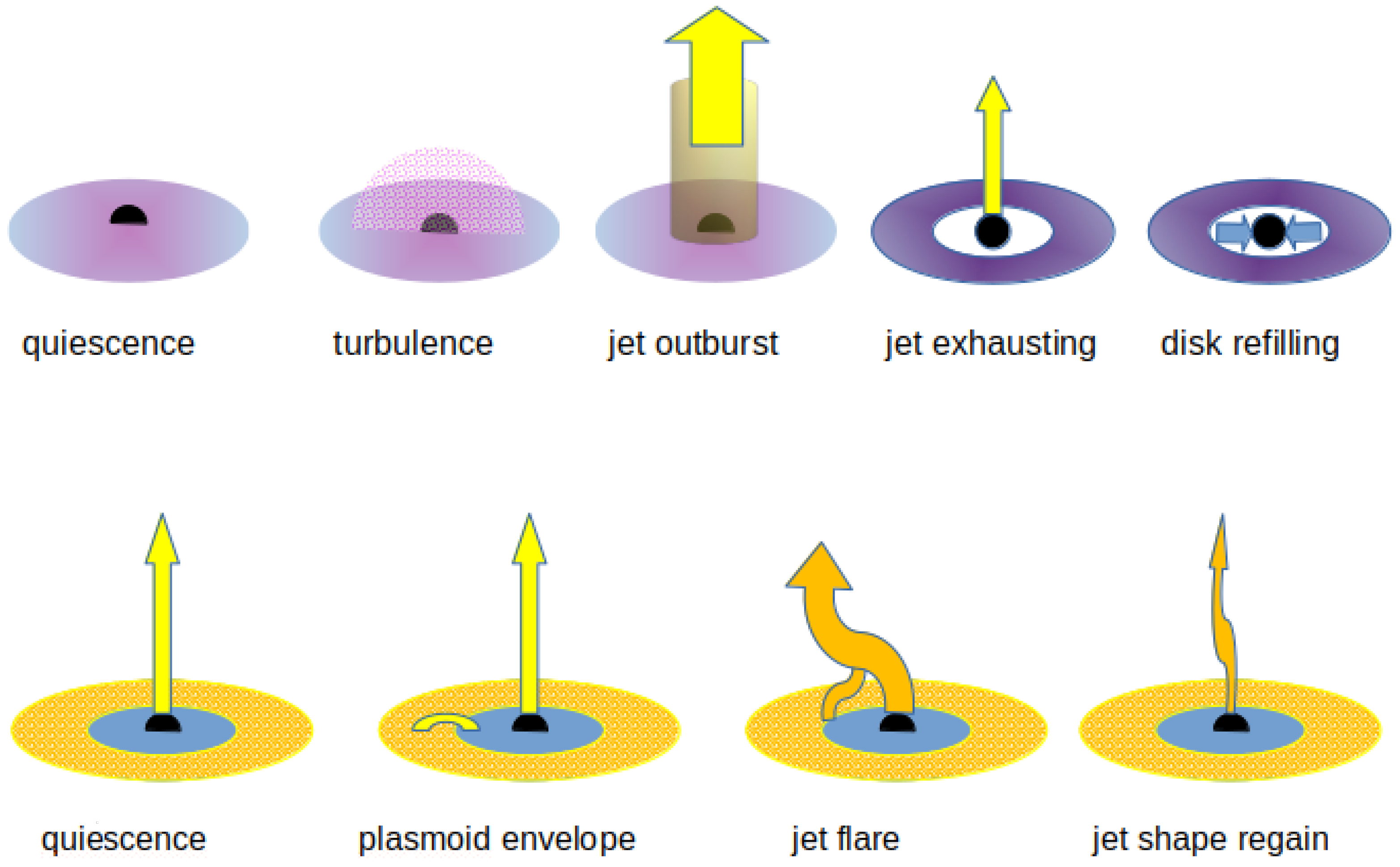
Two main concurring models explain the variability of 3C 120. The first model proposed by Lohfink [7] interprets the wideband variability observed in 3C 120 in terms of the so-called “disk-jet cycle” shown schematically in the upper panel of Figure 1.
The cycle runs from the state of “quiescence” when the disk is “full” (i.e., reaches its inner margin near the central black hole’s innermost stable circular orbit (ISCO) radius or the outer margin of the weak jet base) with no jet (or a weak but stable jet) at the center. Through the turbulent phase, when turbulence arises from the unstable innermost parts of the AGN, it arrives at the outburst state when the jet appears or strengthens significantly. At this point, the central parts of the accretion disk and corona are disrupted, and their matter is pushed away with the powerful jet flow. After reaching its maximum power, the jet gradually exhausts until its initial state, and the stage of disk refilling begins. The physical causes of such a cycle remain open to investigation.
The second model of AGN variability, called the “plasmoid magnetic reconnection”, was proposed by Shukla and Mannheim in [25] for another object, 3C 279, with a similar mechanism proposed to explain the variability of 3C 120 in [26]. The basic assumption of this model lies in the existence of an outer magnetically turbulent zone quite far away from the central black hole, at a distance of about , where enveloped plasmoids can appear and possibly grow if there is an additional fostering factor, such as an external shock wave. Such plasmoids can grow by swallowing smaller plasmoids until the so-called “monster plasmoid” is formed and begins to move inward towards the AGN central black hole. When the monster plasmoid reaches the AGN jet, the magnetic field of the plasmoid reconnects with the jet magnetic field, giving rise to a “jet flare” when the jet is curved and amplified for some period of time. Afterward, the jet exhausts and regains its initial shape. The scheme of this model is shown in the lower panel of Figure 1.
Here, we compare the results of our spectral fitting for 3C 120 with the “jet-disk cycle” and “plasmoid magnetic reconnection” models. To separate the “jet base” spectral component from that of the “disc/corona” one, we use the same two recipes we proposed in [27] for AGN 3C 111. The method is based on the spectral properties of the jet radio synchrotron and X-ray synchrotron self-Compton (SSC) or inverse Compton (IC) emissions. As it was shown in [28], the jet emission spectrum extends from the lower radio frequencies to higher observed energies in the form of the two-humped curve. The interesting property of this curve is that both the upper (IC/SSC) and lower (synchrotron) “knees” have the same photon indices. In case we have the appropriate observational data, we can apply the same power-law photon index value to fit the X-ray SSC/IC and radio synchrotron emission spectra of the jet base. In Section 3.1, we demonstrate the applicability of this method to determine the jet spectral counterparts.
In Section 2, we describe the observational data treated in this work. The basic presumptions of these recipes are described in Section 3.1. In Section 3.2 and Section 3.3, we perform our spectral analysis and compare the results obtained using the recipes mentioned above. In Section 4, we discuss our results, and in Section 5, we draw out our conclusions.
2. Observations and Data Reduction
In our study of 3C 120, we analyzed the X-ray observations performed by XMM-Newton/EPIC, Suzaku/XIS, SWIFT, INTEGRAL, and the Planck observations in radio waves available in the public data archive HEASARC. In this section, we describe the reduction performed to the initial data to obtain the spectra.
All of the soft-to-moderate X-ray data were split into parts corresponding to individual short-time observations (by Suzaku/XIS, XMM-Newton/EPIC and SWIFT/XRT) and fitted individually, to trace out the changes in the spectral shape and the fractions of disc/corona/jet counterparts.
2.1. Planck
We utilized the publicly available Planck spectrum of 3C120 in the 24–240 GHz range from the HEAVENS web page1 from the early release compact source catalog (ERCSC).
2.2. XMM-Newton/EPIC
3C 120 was observed four times by the XMM-Newton mission. The LOG of these observations is shown in Table A1 (Appendix A).
The first two XMM observations of 3C 120, processed in 2002 and 2003, were reduced separately to obtain two complex EPIC spectra for these periods. The spectra obtained from the last two observations, performed shortly after one another in February 2013, were merged into one spectrum.
During all four observational periods, all EPIC cameras were being operated in a partial window mode.
We processed the EPIC data using the XMM SAS version 18.0 software package. The primary data reduction was performed using the standard SAS epproc and emproc chains, taking into account only the single- and double-photon events with the PATTERN ≤ 4 option. We excluded bad pixels and events near the CCD edge using the FLAG filter with FLAG = 0. To extract the source and background counts, we used the 30-radii circular source-centered regions and the empty regions on the same CCD chip with (50–70)-radii, respectively. When creating the spectra, the periods of significant flaring activity were excluded from the cleaned event files using the tabgtigen task. The ancillary files and response matrices were constructed using the standard SAS chains arfgen and rmfgen.
2.3. Swift
The Swift facility’s Burst Alert Telescope (BAT) and X-ray telescope (XRT) observed 3C 120 during the period from 2007 to 2020. We processed the Swift/BAT event and survey data using the BAT sub-packages to obtain spectra in the 14–195 keV energy range for every available period of 3C 120 observations (procedures batbinevt, batupdatephakw and batphasyserr) of the NASA HEASoft version 6.27.22. The whole recipe can be found on the UK Swift Science Data Centre web page3. The corresponding response matrices were generated using the batdrmgen procedure of the same sub-package. To create spectra from detector plane histograms of the BAT survey data, the batdph2pha wasapplied4.
Table A2 (Appendix A) contains the LOG of the Swift/BAT and XRT observations. We merged the closed-in-time observational data (i.e., within a monthly period) and presented them in the same table cell. The total exposure times, count rates, and signal-to-noise ratios for the resulting merged observational periods are also shown.
The Swift/XRT data were reduced using the online software provided by the Department of Physics and Astronomy of the University of Leicester (XROA)5. We utilized the single-pass centroid method with a maximum of 10 attempts and a search radius of 6 arcmin to determine the X-ray source position. Similar to the BAT observations, for the XRT data, the event collections of several close-in-time observations performed within the same months were merged.
2.4. Suzaku
The Suzaku mission performed six observations of 3C 120, four in February–March 2006 and two in February 2012. The LOG of all the Suzaku/XIS observations of 3C 120 is presented in Table A3 (Appendix A).
We reduced the Suzaku/XIS spectra by means of the online multi-mission web-interface UDON2 (Universe via Darts ON-line) provided by the Institute of Space and Astronautical Science (ISAS) by JAXA (Japan Aerospace Exploration Agency). The UDON2 web page and the archived Suzaku observational data can be found publically6. The resulting spectra obtained by UDON2 for all available XIS spectrometers during the same observation were merged into one using the add_asca_spec routine included in the HEASoft 6.26 software package. After this, we merged all the spectra obtained during February–March 2006 into one file with a total exposure time of 165.3 ksec and the two spectra obtained in February 2012 into another spectral file with a total exposure time of 301.1 ksec.
2.5. INTEGRAL
The INTEGRAL/ISGRI observations of 3C 120 were performed during 2005–2020; the observation LOG is shown in Table A4 (Appendix A). The total ISGRI exposure time of the dataset used was 3.96 Ms (including all of the observations when the object was at an angle less than off-axis). To reduce the INTEGRAL IBIS/ISGRI dataset, we used standard recipes from Offline Scientific Analysis (OSA) software, version 11.1. All of the spectra were extracted individually for every science window and then summed up into the sets corresponding to the specific periods of observation times. Moreover, 3C 120 was detected by ISGRI up to the ∼500 keV energy level.
3. Data Analysis
3.1. Distinguishing Nuclear and Jet Base Spectral Components
The main difference between RL and RQ AGN spectra in hard X-rays lies in the presence of the jet base-induced component in the spectra of RL AGN [29]. Another difference is related to the conditions in the central engine, such as a larger inner radius of an accretion disk and a lower coronal temperature in an RL AGN compared to an RQ one [30]. The jets are bright in the radio range, which enables us to distinguish between the jet base and nuclear counterparts in the RL AGN spectra in X-rays as well. We use the same spectral component distinguishing method used in our previous work [27] for 3C 111 and in [31] for a sample of blazars. In [27], we proposed two ways to determine the jet base and primary nuclear counterparts in the X-ray spectrum.
The first way is based on the specific properties of a typical jet spectrum, which consists of two principal components: the low-energy component induced by synchrotron emission of the electrons composing the jet base (from radio to UV), and the high-energy component from UV to the highest -rays due to the IC (inverse Compton) or SSC (synchrotron self-Compton) jet base emissions. The important property of such a spectrum is that it has the same photon index in the radio wave range as in the X-rays [28].
The jet base (of a pc size) is composed of ultra-relativistic charged particles that are ejected from the central region of the AGN at a relativistic bulk velocity. After being accelerated at the wavefront of a shock inside the jet, these particles emit synchrotron radiation that is visible in a wide energy range, from radio to UV. In the local thermodynamic equilibrium, these charged particles follow a power-law distribution with a spectral index of , which generates self-absorbed synchrotron emissions with the following spectral energy distribution (SED):
where is the break frequency at which an optical depth is .
If we consider the energy range above the break energy of our object, i.e., , this formula can be approximated with the simple power-law dependency with the slope , where is the photon index [28,32,33]:
Similarly, within the energy range underlying the break energy we can approximate Formula (1) with the power-law dependency again, but with the spectral index 5/2 (i.e., ). The non-equilibrium configuration of the jet base with the turbulent magnetic field was considered in [34,35,36]; they showed that the peak segments of the SED can sometimes be enlarged to form a plateau, but the “knees” have the same slopes. The slope of the “upper knees” can vary with the electron density or energy distribution, but the “lower knee” is expected to have a persisting slope within the models described above. Taking all of this into account, we can roughly consider both the synchrotron and SSC/IC counterparts of the jet base spectra, consisting of the three following segments:
- Absorbed segment or “lower knee”, power-law with the slope near 1.5;
- Peak or plateau segment near the break energy;
- Transparent segment or “upper knee”, power-law with the slope .
The slopes of the “lower knees” of synchrotron and SSC/IC spectra are the same, as well as the synchrotron and SSC/IC “upper knees” slopes.
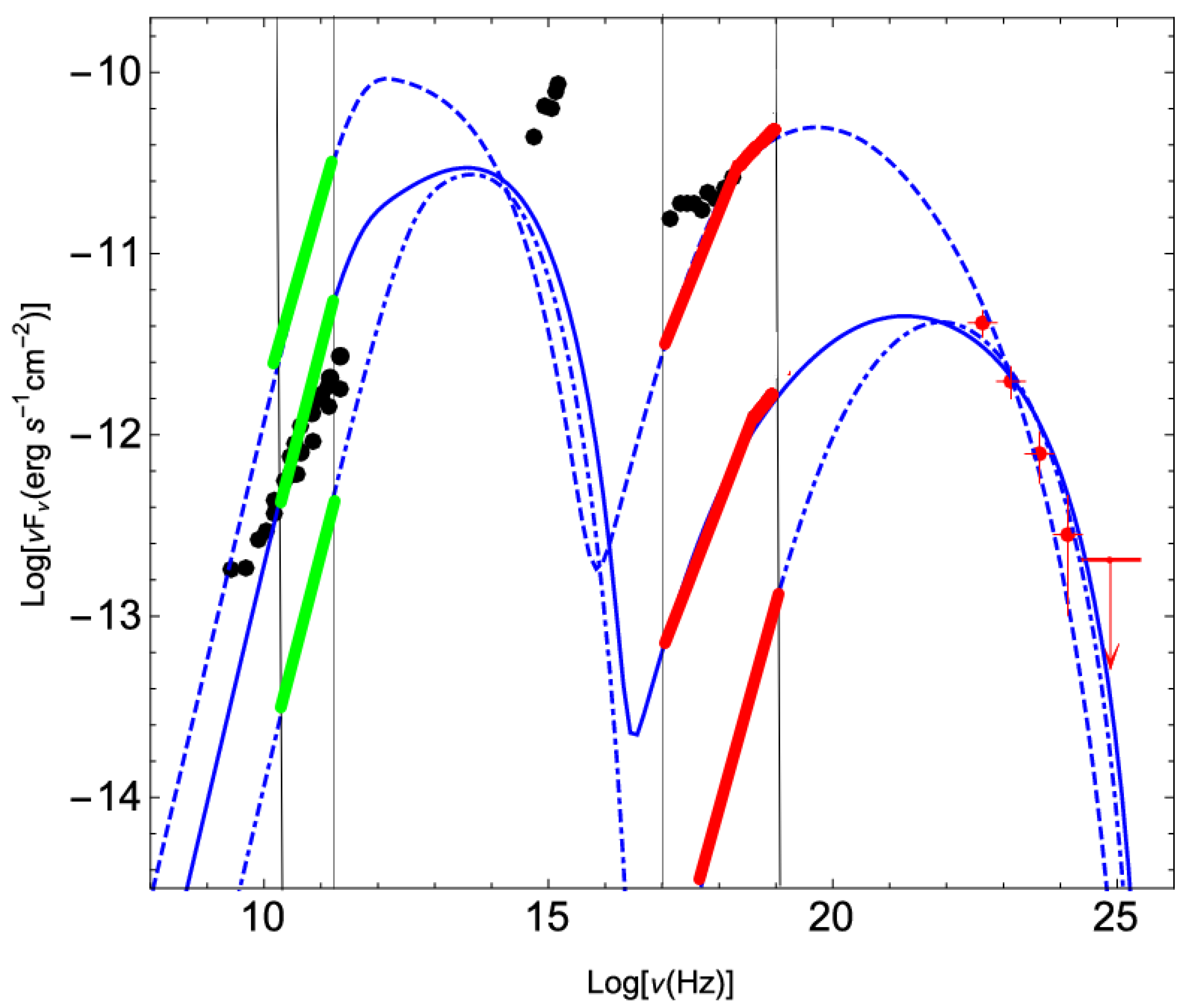
However, before applying this method to a specific object, it is necessary to check its applicability within the working energy intervals of the observational facilities providing the data for the investigation of the object. In our case, we have the 20–240 GHz radio window of Planck, the 3–10 keV energy range of Swift/XRT, XMM-Newton/EPIC, and Suzaku/XIS, and the 15–500 keV range of INTEGRAL/ISGRI and Swift/BAT. To see if we can apply our method, we demonstrate in Figure 2 the SED of 3C 120 within the one-zone SSC model by [37], constructed using the Tramacere SED tool (accessible online at https://www.isdc.unige.ch/sedtool/PROD/SED.html, accessed on 15 December 2021). We plotted the 24–240 GHz Planck working range and 0.1–1000 keV energy range to show that they both cover the “lower knees” areas of synchrotron and SSC/IC jet emissions. Thus, if we assume this model for 3C 120 SED, we can suppose the persistent value of the “lower knee” slope in the radio and X-rays and apply this when fitting the jet base X-ray SSC/IC and radio synchrotron emission spectra. However, as seen from this figure, the “transitional” area, or even the fragment of the “upper knee”, of the SSC/IC jet emission can extend into the 0.1–1000 keV range. For the description of the jet base counterpart in the X-rays, we apply a broken power-law model with a fixed lower photon index and break energy, and a variable upper photon index.
In this view, to separate the contributions of the corona/disk and the jet base, we use the equality of the synchrotron and SSC/IC “lower knee” slopes (), obtained from the Planck 24–240 GHz spectrum of 3C 120. The other two parameters of the X-ray jet base spectral model, the break energy and the upper photon index, are left unfrozen.
The second additional method we are trying here is based on the link between the continuum emission of the corona/disk and the Fe K emission line near 6.4 keV. This line is formed in the accretion disc that is irradiated by the corona and is expected to be correlated with the corona/disk continuum [38]. To understand how this emission line is linked with the primary nuclear continuum, we show a schematic view of the AGN “central engine” and the emission components in Figure 3.
Figure 2.
The radio-to-X-ray data and SED of 3C 120 within the one-zone SSC model by [37], constructed using the Tramacere SED tool. The black circles correspond to observational points from various radio facilities, such as Planck, APEX, ATCA, PACO, SiMPlE, Metsahovi, OVRO, RATAN, UMRAO, and VLA, as well as from Effelsberg, IRAM, KVA, and Xinglong in the IR/optical range, Swift/UVOT in UV rays, and ROSAT/RASS and SWIFT (BAT and XRT) in soft to hard X-rays [39]. The red circles correspond to the Fermi/LAT spectrum. The blue lines (solid, dashed and dotted) show models with different spectral indices. The Planck range is marked by a thick green line, while the X-ray range corresponding to Swift/XRT, XMM-Newton/EPIC, and Suzaku/XIS is marked by red.

In S1 type AGN, such as 3C 120, the observer can detect both the direct and indirect (reflected) emissions from the “central engine.” The direct component originates from the corona and Compton reflection on the accretion disk surface, which gives rise to the broad component of emission lines, such as Fe-K, with specific relativistic profiles. Thus, the two corresponding components in the spectrum are clearly connected. However, the presence of light-bending due to other reflecting elements, such as the torus, can complicate the situation [40,41]. The direct corona continuum, the continuum reflected in the disk, and the line emission can be reflected again in the torus, and there can be additional lines with natural widths emitted in the torus. In the case of a clumpy or patchy torus, the reflection and reprocessing can be very complicated and significantly smear the emission line profiles [42]. Another factor that can affect the situation is the ionization level [43]. If the reflection fraction and ionization level remain constant, one can roughly estimate the link between the line and primary nuclear fluxes as linear. However, in the general case, we should consider the possible variability of the reflection fraction and ionization level, which can be induced by the inhomogeneities in the disk and/or the torus, by the temperature and magnetic field variations, or by the changes of the inner disk radius due to the jet activity. Thus, if we suppose the linear dependence between flux levels in the corona/disk continuum and Fe-K emission line, the parameters of this dependence should take into account the reflector geometry (inclination angle, reflection coefficient, etc.), ionization level, and their variations:
In our case, we cannot establish tight constraints on the inclination value to trace out any variations. However, the variations in the ionization level are clearly visible from the results of the spectral fitting. Here, we are testing if the recipe for determining the nuclear flux based on the iron line is appropriate in such a situation.
Thus, we use the equal “lower knee” slopes for radio synchrotron and X-ray SSC/IC jet base spectral component. The Planck radio spectrum was fitted with a simple power-law model with the photon index . To fit the SSC/IC component in the X-ray spectrum, we used a broken power-law model with the break energy and the photon index of the “upper knee” left free to vary. In addition, we used the linear relationship between the 5–7 keV fluxes in the Fe-K emission line and the continuum component to set up additional constraints on the nuclear disc/corona emission.
3.2. X-ray Spectrum Fitting
We consider the 3.0–300 keV energy range to avoid additional complications due to the presence of the thermal emissions of the gas surrounding the active nucleus in 3C 120, which pollutes its spectra below 3 keV. To fit the 3C 20 hard X-ray spectrum, we used the model containing the following components:
- Fe K 6.4 keV emission line, represented here by the Gaussian model;
- The jet base SSC/IC emission (represented by the broken power-law with no cut-off bknpo model): if and for , with the lower photon index frozen to the value 1.24 obtained from the fitting of the Planck spectrum; the break energy and upper photon index were left free to vary.
The fitting process was performed in the following steps:
- Fitting the 15–300 keV continuum using the cutoffpl model (with the photon index and high-energy exponential cut-off values free to vary) and the broken power-law model for the jet base SSC/IC emission (with the lower photon index frozen to the value 1.24 and break energy and upper photon index free to vary) allows us to obtain constraints on the parameters , , (photon index of the nuclear spectrum), and (high energy exponential cut-off of the primary emission of the nucleus);
- Fitting the 3–300 keV continuum, excluding the 5–7 keV range where the Fe-K emission lines are visible, using the model that includes the jet and the nuclear continuum emission: (xillver-comp()∗high-cut() + bknpo())∗tbabs()∗const with = 1.24 and the other parameters used in the previous step (E, , , E frozen, or confined within the error level to the values obtained in the previous step). Having performed this step, we obtain the values of the thermal (electronic temperature T) and ionization (potential ) parameters of the nuclear continuum, as well as the proper absorption and the fluxes corresponding to the jet and nuclear components;
- The 5–7 keV range fitting using the Gaussian emission line plus the jet and nuclear continuum models with the parameters frozen to the values obtained in the previous steps. The latter gives us the emission line parameters: line energy and width , equivalent width EW, in a 5–7 kev line flux.
We fit the proper and Galactic absorption using the tbabs model, including the Galactic absorption as the lowest possible fitting value at the level of 1.94 × 10 cm [46]. The inter-calibration constants were included in the simultaneous modeling of softer (XMM-Newton/EPIC, Suzaku/XIS, or SWIFT/XRT) and harder (INTEGRAL/ISGRI or Swift/BAT) spectra. Their values were always in the range of 0.6–3.5; they are shown in the last column of Table 1. The lower and upper errors indicated below correspond to the 90% level of confidence (i.e., = 2.71). The standard error calculation algorithm of the HEASoft Xspec software package is as follows: Each non-frozen parameter is varied within its allowed limits until the value of the fit statistic is minimized, which is equal to the last value of the fit statistic determined by the fitting command plus the indicated (i.e., 2.71 in our case). At the end of each table containing the fitting parameters, we also added the variance of the parameter calculated using the following formula:
where P and are the fitting parameter and error bar, and is its mean value.
The spectral modeling was performed by means of the Xspec v.12.12.1f (the HEASoft software package, version 6.30.1). To investigate variability, we combined the Swift/BAT and INTEGRAL spectra from observational time intervals that overlapped with shorter intervals of observations by XMM-Newton/EPIC, Suzaku/XIS, or SWIFT/XRT facilities. The most interesting spectra, along with the fitting spectral models, are shown in Figure A1 in Appendix B.
Initially, all of the observational data were divided into 28 observational periods of monthly duration. However, it was noticed that during the period covering July 2016 to March 2017, the behavior of the primary nuclear counterpart in the spectrum was similar to the photon index at the level of 1.6–1.7, with no detected exponential cut-off at high energies, and the Fe-K emission line was poorly constrained due to insufficient statistics for a high-quality line fit. Therefore, those observational periods, namely December 2012–March 2013, July–September 2016, November–December 2016, and January–March 2017, were merged into longer ones to obtain better constraints on the fitting parameters. This resulted in a set of 20 observational periods described in Table 1. The datasets involving the combination of softer (XMM-Newton/EPIC, SUZAKU/XIS, or SWIFT/XRT) and harder (INTEGRAL/ISGRI or SWIFT/BAT) X-ray spectra were collected during the same periods.
As we can see from Table 1, the values of the photon index corresponding to the “upper knee” of the jet base IC/SSC emissions were mostly compatible with the range of values between 2.0 and 2.8, obtained by [47] from the Fermi/LAT observations of 3C 120. The exceptions were only the two periods with numbers 6 (08/2011) and 16 (11–12/2016) when they were zero-compatible; this can be interpreted as a result of the appearance of the “plateau” in the SSC/IC segment of the jet base emission.
In Table 2, we demonstrate the 3–300 keV continuum parameters obtained in the second step of our fitting, namely the photon index , the high-energy exponential cut-off of the corona/disk continuum, the electronic temperature of the coronal plasma kT, the absorbing column density excess in comparison with the Galactic absorption N, ionization potential , and the /d.o.f. The mean value of the electronic temperature is 17 keV, which is in good agreement with the value of 25 ± 2 keV obtained by [18] from the NuSTAR observations of 3C 120; the temperature itself demonstrates the obvious signs of significant variability, as well as the ionization potential, with variance values of 111.8 and 11.0, correspondingly. The mean values of the photon index and exponential high-energy cut-off in the primary nuclear spectrum are 1.92 ± 0.12 and 72 keV, which are also compatible with the values of 1.87 ± 0.02 (for the photon index) and 83 keV (for the high-energy exponential cut-off) obtained in [18] from the NuSTAR observations within the error levels; the mean value of the photon index of the primary nuclear continuum emission is also compatible with the value of , obtained for 3C 120 in [48]. The higher value of the electronic temperature of the plasma reported in [48], namely keV, is probably due to their model not including the jet base spectral component.
As we can see from our spectral fits during the periods of observation and the plots of their time dependencies shown in Figure A6 and Figure A7 (Appendix D), the parameters of high-energy cut-off and photon index of the primary nuclear emission are highly variable with time, the values of their variances are 344.2 and 28.5; it is noticeable that the values of the upper knee photon index of the jet and that of the primary nuclear continuum are very close to each other. The latter significantly complicates the situation with the jet and nuclear spectral component recognition. It can be seen from Table 2 that the ionization level is, on average, within the range of 3.–4. However, during several periods, it decreased significantly to a level between 2 and 2.2 (or below). We observed three of such periods (9, 15, and 18), with ∼52–54 months period between them.
In Table 3, we present the fitting parameters of the 6.4 keV Fe-K emission line, including the line energy (second column), width (third column), and equivalent width (EW) calculated using the Xspec standard procedure eqwidth (last column). As expected, the variance values of the line energy and width are lower than 1, indicating that these parameters are constant. The flux level and EW, with their variances of 2.27 and 3.67, respectively, show signs of variability during the considered period. The EW values during the observational periods were mostly in the range of 0.03–0.05 keV, typical for RL AGN [49], and compatible with this range within the error levels. However, there was one period (N14, April 2016) when it was significantly higher, at a level of 0.15 keV. Such values of the Fe-K equivalent width are common in RQ AGN [49], which is why we can presume the zero-compatible level of the X-ray jet base emission during this period.
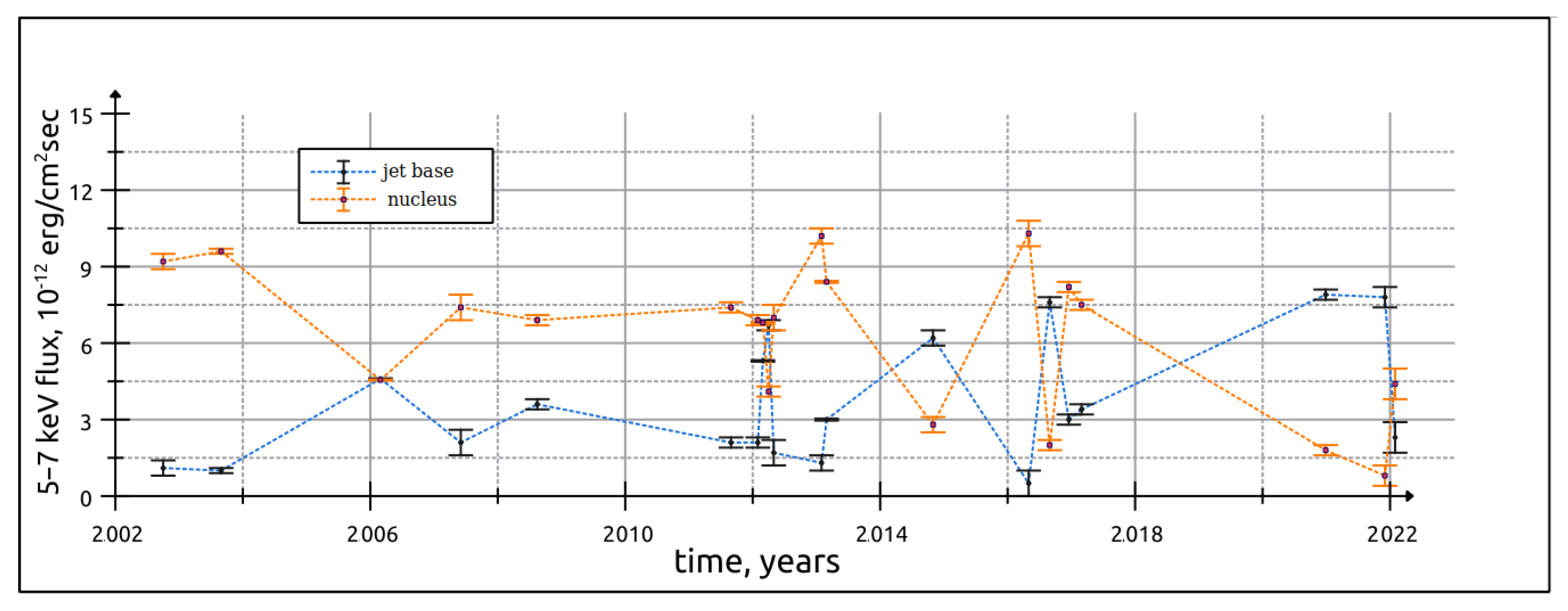
The jet base and corona/disk 5–7 keV continuum fluxes and the 5–7 flux in the Fe-K emission line, calculated using this spectral model, are shown in the Table 4.
3.3. Nuclear Continuum Flux vs. Fe-K Line Flux
In this subsection, we estimate the jet and nuclear 5–7 keV fluxes using the results of the Fe-K emission line fitting, and the emission line fluxes calculated in the previous subsection.
In Figure 4, we arranged equivalent widths of the Fe K line vs. integrated 5–7 keV jet flux to demonstrate that the dependency between them is inverse; for the case of 3C 111, the larger equivalent widths correspond to the smaller values. The highest value of the equivalent width derived for 3C 120 is about 150 eV (14th period) and it corresponds to zero-compatibly or an extremely low level of the jet base emission. This is also in good agreement with the typical values of the EW of RQ AGNs [49].
Now, let us consider the relation between the X-ray continuum in the 5–7 keV range and flux in the Fe K line. Namely, we suppose that the total integrated (5–7 keV) observed flux in the Fe K line is proportional to the total nucleus (disc/corona) flux in the 5–7 keV range: .
We used the results of our spectral fitting in order to derive these coefficients. There was a zero-compatible jet emission period, namely the 14th one. We considered this period to estimate the coefficient’s value of . With this coefficient, we applied it to the data to derive the Fe-K line fluxes to derive the nuclear and jet base fluxes within the 5–7 keV energy range, as shown in Table 4.
Using the linear coefficient found in this recipe, we calculated the values of the nuclear flux for each observation and compared these values with those obtained from the spectral fitting. However, it was observed that the error bars for the fluxes derived with this recipe for 3C 120 were too high to use successfully with the available data for this object.
3.4. Correlation of Parameters
To trace out possible links between the spectral parameters, we calculated the correlations between the fitting parameters , , , , , , lg, EW, and 5–7 keV fluxes corresponding to the jet base, Fe-K emission line, and nuclear counterparts. The correlation between parameters X and Y was calculated using the following formula:
where is the mean value of the X parameter. The positive (+) and negative (−) errors of the correlation coefficients were calculated using the formulae:
where is the positive direction error in the ith observation.
The results are shown in Table 5. As one can notice, there is a correlation between the high-energy exponential cut-off and the electronic temperature in the spectral counterpart corresponding to the primary nuclear (accretion disk + corona) emission, with a coefficient of 0.99; their time dependencies are shown in Figure A7 in Appendix D, demonstrating prominent signs of synchronized variability during the observational period). There is a strong anti-correlation between jet and nuclear fluxes (at the level of −0.9), which can be considered a sign of the close spatial proximity of these two components (i.e., it favors the “jet/disk cycle” rather than the “reconnection” scenario). There is also moderate anti-correlation between the ionization parameter and the jet flux level (−0.74). The 5–7 keV nuclear and jet base flux curves are shown in Figure A6 in Appendix D. Surprisingly, the correlation between the nuclear and Fe-K 5–7 keV emission fluxes was not traced, being at the level of 0.42; this can be considered a result of the ionization level variability [43]. The dependence of the ionization parameter upon the time is shown in Figure 5.
We plotted the dependencies of the parameters with high correlation/anti-correlation levels in Figure 6, Figure 7 and Figure 8; the other pairs with no prominent correlation are shown in Appendix C in Figure A2–Figure A5. As we can see from Figure 6, the dependency between these parameters looks almost linear with the coefficient between these two parameters determined as 3.04 using the minimum squares method; similar values of the coefficient 2.2–5.96 were predicted for 3C 120 in [50].
4. Discussion
We applied the two recipes, giving us the possibility to distinguish between the disk/corona and the jet base contributions to the hard X-ray spectra of the RT AGN 3C 120 proposed in our previous work [27]. We analyzed the data of the XMM-Newton, INTEGRAL, SWIFT, and Suzaku observations during the 20 periods together with the radio data observed by the Planck mission. To perform this separation with the first recipe, we assumed the same values of the photon indices for the lower knees of the X-ray IC/SSC and the radio synchrotron jet base emission spectra of 3C 120 (taking into account that the radio emissions were pure jet base synchrotron emissions). The first method shows quite accurate results, despite the fact that the Planck radio spectrum used to fix the synchrotron emission photon index was averaged over time.
The other recipe we tried to use was based on the link between the emission fluxes of the disk/corona continuum and Fe K line emissions [51,52]. The relative errors of the emission line parameters were too large in most observations, including the 14th one when the jet base emissions were estimated as zero-compatible, which resulted in very rough estimates of the linear coefficient and nuclear fluxes. Additionally, the ionization level in 3C 120 appears to vary significantly over time, breaking the linearity of the link between the Fe-K line and disk/corona continuum fluxes (the variance of the ionization parameter is 11.0). This is confirmed by the results of our correlation analysis (corr(,) = 0.42 is not enough to trace out the correlation). Thus, we can see that this second recipe is rather inappropriate for the case of 3C 120 as it can give us only the lower limit on the primary nuclear emission flux. However, taking into account the close values of the photon indices of the primary nuclear emission and the jet base spectra “upper knee”, the emission line presence during some period of time can be considered as a sign of the primary nuclear emission dominating in the spectrum.
We compare our results with the “disk-jet cycle” model [7] and the “plasmoid magnetic reconnection” model [25]. Following the “disk-jet cycle” model, the structural changes observable in an RT AGN can be interpreted in terms of the five-phase jet-disc cycle:
- Silent full-disc phase: The jet is weak or absent, the disc continues into its innermost stable orbit, and an object looks similar to a classical RQ AGN with prominent emission lines and high values (i.e., above 100 keV) of exponential high-energy cut-off in the corona/disk continuum;
- Phase of instability: The inner part of the disc becomes unstable, ionized, and/or heated, turbulent, and radiatively inefficient, causing luminescent Fe-K lines to weaken. At the same time, recombination lines of strongly ionized iron, such as the 6.58 keV Fe XXII and 6.64 keV Fe XXIV, can appear. During this phase, lower values of high-energy exponential cut-off in the primary nuclear continuum (below 100 keV) can be observed, and jet appearances are still weak or even absent;
- Jet outburst: Jet power increases rapidly and significantly. During this phase, the jet emission dominates, whereas the nuclear continuum can be invisible or weak in comparison with the jet component, with the exponential cut-off below 100 keV. The emission lines are weak as well. AGN looks similar to a typical RL at this stage;
- Jet exhausting: The jet power gradually decreases to the “normal” value or even lower. During this phase, the jet emission is no longer dominant, and the nuclear continuum can be at a similar level, with the exponential cut-off below 100 keV. The emission lines are typically weak at this stage;
- Disc refilling: The accretion disc begins to refill. During this phase, the AGN can look similar to an RQ AGN again. It can be characterized by the “weakness” of all of its counterparts: the flux from the jet base is zero-compatible, the iron K lines are weak (if present), and the exponential cut-off in the primary nuclear continuum is below 100 keV.
Within this model, there are no direct correlations between the flux levels (for the jet base emission or the primary nuclear one) and high-energy exponential cut-off or electronic temperature values. As for the ionization level, it should anti-correlate with the jet base flux (as lower ionization levels can indicate that the central regions of the disc/corona are disrupted by the jet outburst). It can optionally correlate with the primary nuclear flux. The nuclear and jet base fluxes, being fed from the same source (region), are supposed to be anti-correlated.
The “plasmoid magnetic reconnection” model predicts the following four phases:
- Quiescence: The jet is weak with its normal flux values; within the outer magnetically turbulent zone, there are small-scale plasmoids that form;
- Plasmoid envelope: The “monster” plasmoid forms and begins to move inwards down to the central black hole;
- Jet flare: The “monster” reconnects to the jet, inflicting the fast and significant growth of the jet power and curving the jet;
- Jet shape regain: The jet power gradually returns to its “quiescent” values; the jet itself regains its initial (i.e., direct) shape.
Within this model, there are no direct correlations between the flux levels and the high-energy exponential cut-off or electronic temperature. There is no correlation between the jet flux and nuclear flux, but there may be a correlation with the ionization level. Additionally, a curved jet can play a role in providing seed photons for the Fe-K emission lines that are Compton-reflected from the accretion disc surface.
As we can see from Table 3, the jet flux anti-correlates with the ionization level (see Figure 7) and with the primary nuclear flux. That is why we can say that our results favor the “jet-disc cycle” model.
However, there is still an interesting question that remains unanswered: what are the physical reasons causing such structural changes in the “central engine” of an RT AGN? A possible explanation for this structural instability could include some quite exotic alternatives to a central massive black hole, such as wormholes, “magnetic tunnels” [53,54], or weakly/strongly naked singularities [55].
A stream of charged particles passing through a “magnetic tunnel” would cause the appearance of a magnetic field around it, resulting in a “silent phase”. Due to the “Lorentz ionization effect” [56], the ionization level of the disc/corona would increase along with the magnetic field of the central object during the “turbulent phase”. When the magnetic field is strong enough, it launches jets during the “jet activity phase”, which takes away the disc plasma and interrupts its inflow into the tunnel. After the interruption of the jets, the disc remains truncated and begins to refill during the “refilling phase”.
A more accurate determination of the profiles of the emission lines formed in the near vicinity of the central object of the AGN can give us the possibility to test such exotic models [57].
Another important clue to understanding the scenarios of jet formation in this object and to determine the jet composition (i.e., hadronic or leptonic) lies at the highest energy ranges, leading to key information about their spectra above 10–10 eV [58]. Tracing out this difference can be performed in a more effective way by combining the existing Fermi-LAT observational data with the Cherenkov Telescope Array (CTA) results [59].
5. Conclusions
- We applied the recipes proposed in [27] to separate the “jet base” and “central engine” spectral components in the case of AGN 3C 120 in the range from X-ray to soft -ray spectrum for 20 periods of observations by Suzaku/XIS, XMM-Newton/EPIC, SWIFT, and INTEGRAL/ISGRI. Despite the close values of the photon indices corresponding to the jet base and primary nuclear emission, the results of the distinguishing components look optimistic enough.
- Our fitting results are in good agreement with the “jet-disc cycle” model [7].
- The maximal values of the Fe K line-equivalent widths obtained during the “silent” phases are in satisfactory agreement with the values typical for RQ AGN.
Author Contributions
E.F.: data processing, fitting and analysis; A.D.P.: paper writing and text editing. All authors have read and agreed to the published version of the manuscript.
Funding
This research received no external funding.
Data Availability Statement
The reduced observational data and fitting results are available from the authors.
Acknowledgments
We are grateful to the anonymous reviewers for their very attentive and helpful comments and suggestions, which helped us significantly improve the quality of the manuscript. E.F is thankful to Bohdan I. Hnatyk for his useful discussions on the matter.
Conflicts of Interest
The authors declare no conflict of interest.
Sample Availability
The reduced data samples and fitting results are available from the authors.
Appendix A. Observations LOG

Table A1.
The XMM-Newton/EPIC observational LOG. The data events from various data merged to produce one common spectrum, shown in one cell; the results of merging them are marked as “total”.
Table A1.
The XMM-Newton/EPIC observational LOG. The data events from various data merged to produce one common spectrum, shown in one cell; the results of merging them are marked as “total”.
| obsID | Obs. | Obs. Time, | Total EPIC |
|---|---|---|---|
| Date | ks | Flux, cts | |
| 0109131101 | 2002-09-06 | 11.9 | 262,349 |
| 0152840101 | 2003-08-26 | 123.5 | 1,275,340 |
| 0693781601 | 2013-02-06 | 52.9 | 1,271,861 |
| 0693782401 | 2013-02-08 | 27.7 | 743,677 |
| total | 2013-02 | 80.6 | 2015538 |
Table A2.
SWIFT XRT and BAT observation LOG.
| Obs. | XRT Exp., | XRT Flux | XRT Mode | BAT Exp. | BAT Flux |
|---|---|---|---|---|---|
| Date | ks | cts | ks | cts | |
| 2007 | 10.7 | 623 | pc | 9.5 | 0 |
| 2008 | 26.4 | 1411 | pc | 26.4 | 0 |
| 2011 | 14.2 | 1910 | pc | 14.2 | 0 |
| 2012/01 | 14.2 | 1712 | pc | 14.2 | 290 |
| 2012/02 | 9.7 | 1808 | wt | 9.2 | 650 |
| 2012/03 | 14.3 | 1852 | wt | 14.3 | 106 |
| 2012/04 | 6.7 | 975 | pc/wt | 6.7 | 0 |
| 2012/12 | 9.7 | 3074 | pc/wt | 4.3 | 0 |
| 2013/01 | 18.3 | 2044 | pc/wt | 4.4 | 200 |
| 2013/02 | 22.8 | 2046 | pc/wt | 14.8 | 490 |
| 2013/03 | 10.8 | 5798 | pc/wt | 10.9 | 90 |
| 2014/10 | 4.2 | 679 | wt | 4.3 | 0 |
| 2016/04 | 9.3 | 1272 | pc/wt | 9.5 | 110 |
| 2016/07 | 8.8 | 960 | wt | 8.8 | 150 |
| 2016/08 | 16.1 | 2015 | pc/wt | 16.3 | 680 |
| 2016/09 | 10.9 | 1500 | wt | 10.5 | 300 |
| 2016/10 | 10.2 | 1600 | wt | 12.3 | 480 |
| 2016/11 | 12.2 | 1600 | wt | 11.9 | 520 |
| 2016/12 | 12.0 | 1500 | wt | 11.5 | 360 |
| 2017/01 | 11.7 | 1991 | wt | 11.4 | 1390 |
| 2017/02 | 13.2 | 2021 | wt | 12.9 | 1570 |
| 2017/03 | 12.8 | 2200 | wt | 11.2 | 1550 |
| 2018/03 | 1.0 | 330 | pc | 1.0 | 100 |
| 2020 | 26.0 | 4246 | wt | 27.6 | 420 |
Table A3.
Suzaku/XIS observation LOG. The data events from various data shown in one cell were merged to produce one common spectrum, marked as “total”.
Table A3.
Suzaku/XIS observation LOG. The data events from various data shown in one cell were merged to produce one common spectrum, marked as “total”.
| obsID | Obs. | Obs. Time, | Total Flux |
|---|---|---|---|
| Date | ks | cts | |
| 700001010 | 2006-02-09 | 41.9 | 448,401 |
| 700001020 | 2006-02-16 | 41.6 | 350,606 |
| 700001030 | 2006-02-23 | 40.9 | 417,900 |
| 700001040 | 2006-03-02 | 40.9 | 360,368 |
| Total | 165.3 | 1,577,275 | |
| 706042010 | 2012-02-09 | 183.0 | 1,581,225 |
| 706042020 | 2012-02-14 | 118.1 | 1,020,452 |
| Total | 301.1 | 2,601,677 |
Table A4.
INTEGRAL/ISGRI observation LOG.
| Data | Obs. | Obs. Time, | Data | obs. | Obs. Time, | Data | Obs. | Obs. Time, |
|---|---|---|---|---|---|---|---|---|
| rev | Date | ks | rev | Date | ks | rev | Date | ks |
| 0338 | 2005-07 | 1.1 | 1378 | 2014-01 | 30.0 | 2070 | 2019-03 | 10.0 |
| 0343 | 2005-08 | 79.0 | 1379 | 2014-01 | 63.0 | 2076 | 2019-04 | 13.0 |
| 0344 | 2005-08 | 183.0 | 1439 | 2014-07 | 3.4 | 2121 | 2019-08 | 175.0 |
| 0346 | 2005-08 | 112.0 | 1441 | 2014-08 | 102.3 | 2123 | 2019-08 | 168.0 |
| total | 375.1 | 1442 | 2014-08 | 171.0 | 2124 | 2019-08 | 113.5 | |
| 0483 | 2006-09 | 49.0 | 1444 | 2014-08 | 15.0 | 2126 | 2019-08 | 14.0 |
| 0487 | 2006-10 | 63.0 | 1445 | 2014-08 | 3.5 | 2127 | 2019-08 | 10.0 |
| total | 112.0 | 1446 | 2014-08 | 13.0 | 2136 | 2019-09 | 13.0 | |
| 0530 | 2007-01 | 17.0 | 1447 | 2014-08 | 75.0 | 2137 | 2019-09 | 20.5 |
| 0532 | 2007-02 | 57.8 | 1456 | 2014-08 | 5.3 | 2143 | 2019-10 | 175.0 |
| 0538 | 2007-03 | 64.6 | 1457 | 2014-09 | 49.0 | 2148 | 2019-10 | 20.0 |
| 0543 | 2007-03 | 25.5 | 1459 | 2014-09 | 15.0 | total | 731.5 | |
| 0548 | 2007-04 | 36.0 | 1463 | 2014-10 | 6.5 | 2187 | 2020-01 | 153.5 |
| 0588 | 2007-08 | 4.0 | total | 552.0 | 2188 | 2020-01 | 189.5 | |
| 0589 | 2007-08 | 70.0 | 1503 | 2015-02 | 92.4 | 2189 | 2020-02 | 180.0 |
| 0590 | 2008-08 | 57.8 | 1504 | 2015-02 | 8.8 | 2194 | 2020-02 | 6.6 |
| 0591 | 2008-08 | 57.8 | 1505 | 2015-02 | 10.0 | 2198 | 2020-02 | 22.4 |
| total | 373.5 | 1520 | 2015-03 | 31.0 | total | 552.0 | ||
| 0650 | 2008-02 | 22.2 | 1523 | 2015-03 | 33.0 | 2210 | 2020-03 | 19.2 |
| 0656 | 2008-02 | 68.0 | 1524 | 2015-03 | 37.0 | 2212 | 2020-04 | 19.3 |
| 0659 | 2008-03 | 52.5 | 1528 | 2015-03 | 16.0 | 2217 | 2020-04 | 33.0 |
| total | 142.7 | 1575 | 2015-08 | 20.0 | total | 52.3 | ||
| 1073 | 2011-07 | 6.5 | 1577 | 2015-08 | 54.0 | 2257 | 2020-07 | 75.6 |
| 1075 | 2011-08 | 1.1 | 1581 | 2015-09 | 45.5 | 2258 | 2020-08 | 73.6 |
| 1077 | 2011-08 | 1.0 | 1584 | 2015-09 | 30.0 | 2259 | 2020-08 | 67.2 |
| total | 8.6 | 1593 | 2015-09 | 34.0 | 2260 | 2020-08 | 83.2 | |
| 1252 | 2013-01 | 1.2 | total | 411.7 | 2261 | 2020-08 | 52.5 | |
| 1254 | 2013-01 | 1.1 | 1644 | 2016-02 | 59.5 | 2263 | 2020-08 | 13.2 |
| 1256 | 2013-01 | 23.0 | 1660 | 2016-03 | 21.0 | 2265 | 2020-08 | 59.4 |
| 1257 | 2013-01 | 13.0 | 1664 | 2016-04 | 28.0 | 2266 | 2020-08 | 59.4 |
| 1258 | 2013-02 | 135.0 | total | 108.5 | 2267 | 2020-08 | 89.6 | |
| 1259 | 2013-02 | 135.0 | 1781 | 2017-02 | 3.5 | total | 484.1 | |
| 1260 | 2013-02 | 3.3 | 1794 | 2017-03 | 17.0 | 2269 | 2020-09 | 79.2 |
| 1264 | 2103-02 | 23.3 | 1801 | 2017-04 | 13.0 | 2270 | 2020-09 | 73.5 |
| 1270 | 2013-03 | 15.0 | total | 33.5 | total | 152.7 | ||
| 1275 | 2013-03 | 1.3 | 1921 | 2018-02 | 3.3 | |||
| 1278 | 2013-04 | 10.0 | 1925 | 2018-03 | 3.3 | |||
| 1279 | 2013-04 | 40.0 | 1930 | 2018-03 | 9.7 | |||
| 1281 | 2013-04 | 5.6 | 1941 | 2018-04 | 20.0 | |||
| 1316 | 2013-07 | 18.0 | 1978 | 2018-07 | 1.0 | |||
| 1317 | 2013-07 | 25.0 | 1987 | 2018-08 | 8.3 | |||
| 1326 | 2013-08 | 23.0 | 1991 | 2018-09 | 6.5 | |||
| 1329 | 2013-09 | 6.7 | 1996 | 2018-09 | 6.5 | |||
| 1330 | 2013-09 | 19.2 | 2010 | 2018-10 | 13.0 | |||
| 1331 | 2013-09 | 59.5 | 2011 | 2018-10 | 25.6 | |||
| 1332 | 2013-09 | 59.5 | total | 123.7 | ||||
| 1333 | 2013-09 | 11.0 | ||||||
| 1338 | 2013-09 | 24.5 | ||||||
| total | 453.2 |
Appendix B. Spectra and Fits
Figure A1.
The XMM-Newton/EPIC (the upper left panel: black line—MOS cameras, red line—PN camera), Suzaku/XIS (the upper right and lower left panel, black line), INTEGRAL: JEM-X (the upper left panel: blue line, the upper right panel: red line) and ISGRI (the upper left panel: cyan line, the upper right and lower left panels: green line), Swift: XRT (the lower left panel: red line, the lower right panel: black line) and BAT (the upper left panel: green line, the lower left panel: blue line, the lower right panel: red line) unfolded spectra, and fitting model of 3C 120 during the observation, 2/August 2003 (upper left panel), 3/February 2006 (upper right panel), 8/February 2012 (bottom left panel), and 19/November 2021 (bottom right panel).

Appendix C. Correlation of the Spectral Fitting Parameters
Figure A2.
Absorbing column N, 10 cm vs. photon index of the primary nuclear emission.

Figure A3.
The high-energy exponential cut-off vs. photon index in the primary nuclear emission spectrum of 3C 120.
Figure A3.
The high-energy exponential cut-off vs. photon index in the primary nuclear emission spectrum of 3C 120.

Figure A4.
Ionization level lg vs. photon index of the primary nuclear emission of 3C 120.

Figure A5.
Break energy vs. upper photon index in the jet base spectrum.

Appendix D. Dependencies of the Fitting Parameters on the Time
Figure A6.
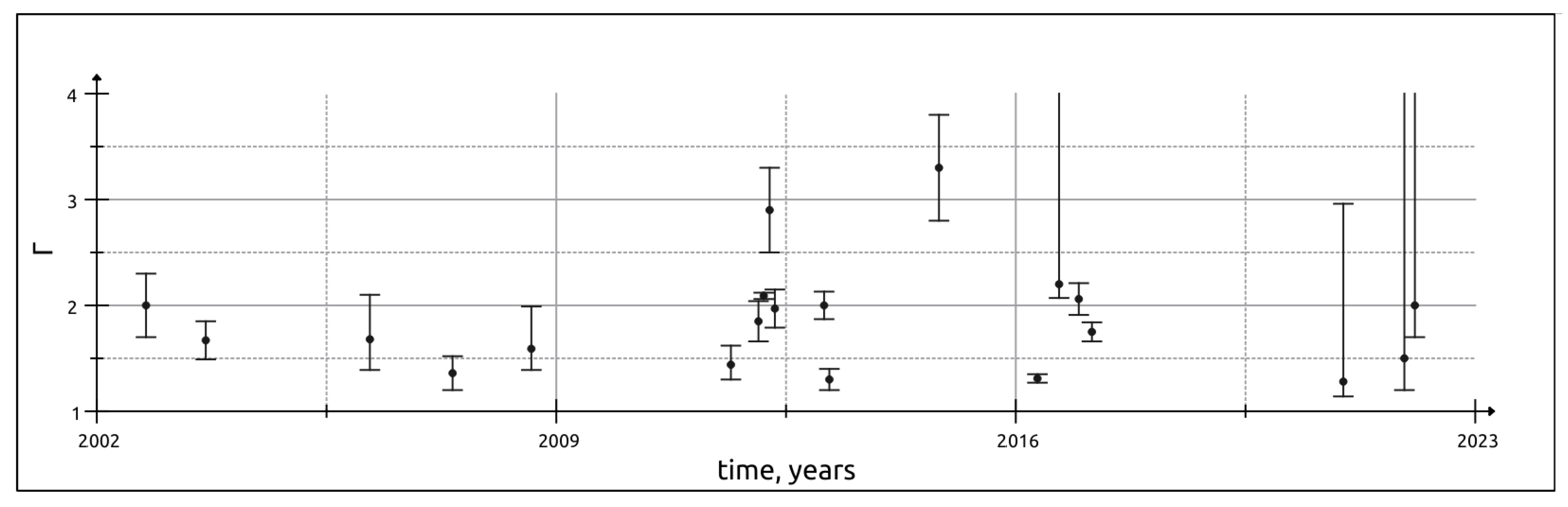
The dependence of the photon index of the primary nuclear emission in 3C 120 on the time.
Figure A6.
The dependence of the photon index of the primary nuclear emission in 3C 120 on the time.

Figure A7.
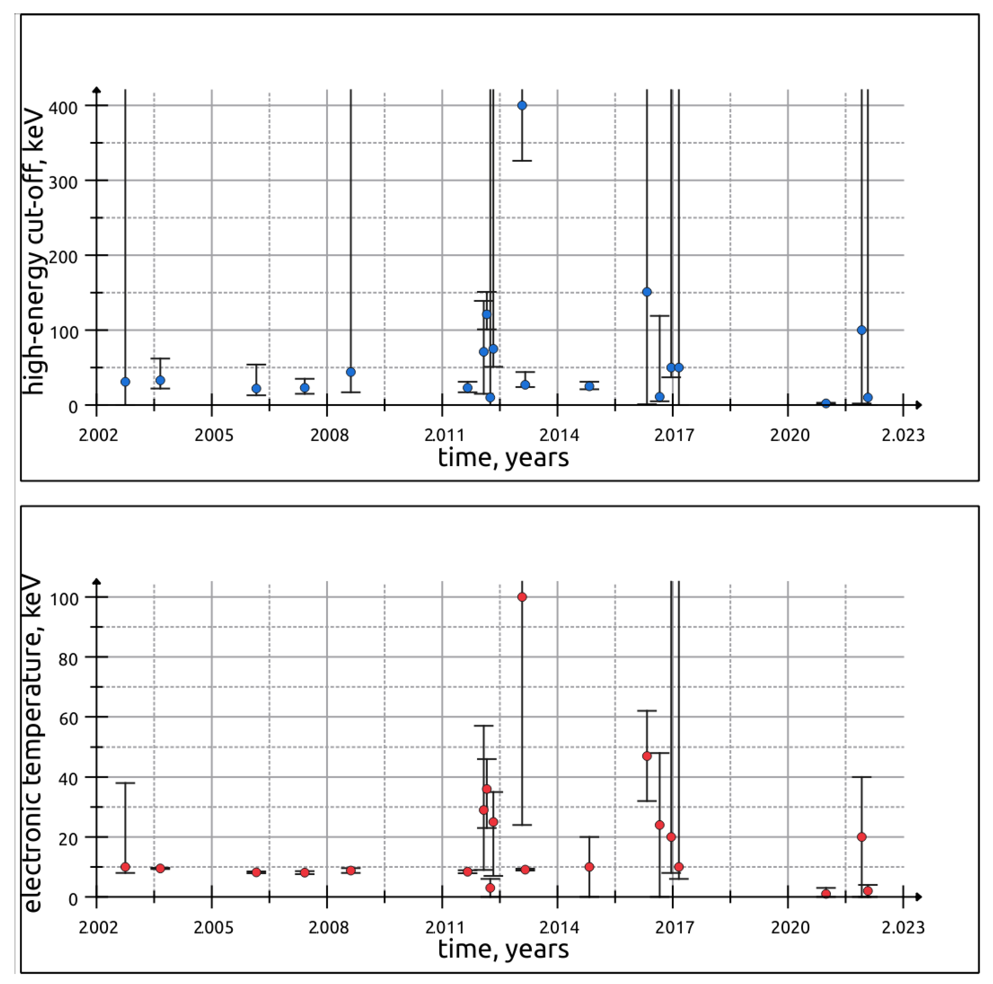
The dependencies of the electronic temperature of the plasma in the corona and the high-energy exponential cut-off in the primary nuclear emission spectrum of 3C 120 on the time.
Figure A7.
The dependencies of the electronic temperature of the plasma in the corona and the high-energy exponential cut-off in the primary nuclear emission spectrum of 3C 120 on the time.

Figure A8.
Jet base (black squares) and primary nuclear (red circles) flux curves.

| 1 | https://www.isdc.unige.ch/heavens, accessed on 5 July 2021. |
| 2 | https://heasarc.gsfc.nasa.gov/lHEASoft/, accessed on 15 September 2022. |
| 3 | https://www.swift.ac.uk/analysis/bat/spectra.php, accessed on 3 March 2023. |
| 4 | https://heasarc.gsfc.nasa.gov/lHEASoft/ftools/headas/batdph2pha.html, accessed on 15 September 2022. |
| 5 | https://www.swift.ac.uk/, accessed on 11 October 2022. |
| 6 | https://darts.isas.jaxa.jp/astro/udon2/udon2-usage/, accessed on 3 March 2023. |
References
- Kellermann, K.I.; Sramek, R.; Schmidt, M.; Shaffer, D.B.; Green, R. VLA Observations of Objects in the Palomar Bright Quasar Survey. Astron. J. 1989, 98, 1195. [Google Scholar] [CrossRef]
- Sulentic, J.W.; Marziani, P.; Dultzin, D.; D’Onofrio, M.; del Olmo, A. Fifty Years of Quasars: Physical Insights and Potential for Cosmology. J. Phys. Conf. Ser. 2014, 565, 012018. [Google Scholar] [CrossRef]
- Chen, L.; Bai, J.M.; Zhang, J.; Liu, H.T. Possible γ-ray emission of radio intermediate AGN III Zw 2 and its implication on the evolution of jets in AGNs. Res. Astron. Astrophys. 2010, 10, 707–712. [Google Scholar] [CrossRef]
- Pierce, J.C.S.; Tadhunter, C.N.; Ramos Almeida, C.; Bessiere, P.S.; Rose, M. Do AGN triggering mechanisms vary with radio power?—I. Optical morphologies of radio-intermediate HERGs. Mon. Not. R. Astron. Soc. 2019, 487, 5490–5507. [Google Scholar] [CrossRef]
- Mundell, C.G.; Ferruit, P.; Nagar, N.; Wilson, A.S. Radio Variability in Seyfert Nuclei. Astrophys. J. 2009, 703, 802–815. [Google Scholar] [CrossRef]
- Shulevski, A.; Morganti, R.; Barthel, P.D.; Murgia, M.; van Weeren, R.J.; White, G.J.; Brüggen, M.; Kunert-Bajraszewska, M.; Jamrozy, M.; Best, P.N.; et al. The peculiar radio galaxy 4C 35.06: A case for recurrent AGN activity? Astron. Astrophys. 2015, 579, A27. [Google Scholar] [CrossRef] [Green Version]
- Lohfink, A.M.; Reynolds, C.S.; Jorstad, S.G.; Marscher, A.P.; Miller, E.D.; Aller, H.; Aller, M.F.; Brenneman, L.W.; Fabian, A.C.; Miller, J.M.; et al. An X-Ray View of the Jet Cycle in the Radio-loud AGN 3C120. Astrophys. J. 2013, 772, 83. [Google Scholar] [CrossRef]
- Marscher, A.P. Relativistic Jets in Blazars: Where the Action Is. In Proceedings of the Radio Astronomy at the Fringe; Astronomical Society of the Pacific Conference Series; Zensus, J.A., Cohen, M.H., Ros, E., Eds.; Astronomical Society of the Pacific: San Francisco, CA, USA, 2003; Volume 300, p. 133. [Google Scholar]
- Lavaux, G.; Hudson, M.J. The 2M++ galaxy redshift catalogue. Mon. Not. R. Astron. Soc. 2011, 416, 2840–2856. [Google Scholar] [CrossRef]
- Vorontsov-Vel’Yaminov, B.A.; Arkhipova, V.P. Morphological catalogue of galaxies. Part III. Catalogue of 6740 galaxies between declinations +15 and −9. Trudy Gos. Astron. Inst. 1963, 33, 1–260. [Google Scholar]
- Balick, B.; Heckman, T.M.; Crane, P.C. The large-scale radio structure of 3C 120. Astrophys. J. 1982, 254, 483–488. [Google Scholar] [CrossRef]
- Gómez, J.L.; Marscher, A.P.; Alberdi, A. 86, 43, and 22 GHz VLBI Observations of 3C 120. Astrophys. J. 1999, 521, L29–L32. [Google Scholar] [CrossRef] [Green Version]
- Pozo Nu nez, F.; Ramolla, M.; Westhues, C.; Bruckmann, C.; Haas, M.; Chini, R.; Steenbrugge, K.; Murphy, M. Photometric reverberation mapping of 3C 120. Astron. Astrophys. 2012, 545, A84. [Google Scholar] [CrossRef] [Green Version]
- Ballantyne, D.R.; Fabian, A.C.; Iwasawa, K. The XMM-Newton view of the broad-line radio galaxy 3C 120. Mon. Not. R. Astron. Soc. 2004, 354, 839–850. [Google Scholar] [CrossRef] [Green Version]
- Tombesi, F.; Mushotzky, R.F.; Reynolds, C.S.; Kallman, T.; Reeves, J.N.; Braito, V.; Ueda, Y.; Leutenegger, M.A.; Williams, B.J.; Stawarz, Ł.; et al. Feeding and Feedback in the Powerful Radio Galaxy 3C 120. Astrophys. J. 2017, 838, 16. [Google Scholar] [CrossRef] [Green Version]
- Kataoka, J.; Reeves, J.N.; Iwasawa, K.; Markowitz, A.G.; Mushotzky, R.F.; Arimoto, M.; Takahashi, T.; Tsubuku, Y.; Ushio, M.; Watanabe, S.; et al. Probing the Disk-Jet Connection of the Radio Galaxy 3C 120 Observed with Suzaku. Publ. Astron. Soc. Jpn. 2007, 59, 279–297. [Google Scholar] [CrossRef] [Green Version]
- Fedorova, E.; Vasylenko, A.; Zhdanov, V. Peculiar AGNs from the INTEGRAL and RXTE data. Bull. Taras Shevchenko Natl. Univ. Kyiv Astron. 2017, 55, 29–34. [Google Scholar] [CrossRef] [Green Version]
- Rani, P.; Stalin, C.S. Coronal Proerties of the Seyfert 1 Galaxy 3C 120 with NuSTAR. Astrophys. J. 2018, 856, 120. [Google Scholar] [CrossRef] [Green Version]
- Zargaryan, D.; Gasparyan, S.; Baghmanyan, V.; Sahakyan, N. Comparing 3C 120 jet emission at small and large scales. Astron. Astrophys. 2017, 608, A37. [Google Scholar] [CrossRef] [Green Version]
- Zdziarski, A.A.; Egron, E. What are the Composition and Power of the Jet in Cyg X-1? Astrophys. J. 2022, 935, L4. [Google Scholar] [CrossRef]
- Marscher, A.P.; Jorstad, S.G.; Gómez, J.L.; Aller, M.F.; Teräsranta, H.; Lister, M.L.; Stirling, A.M. Observational evidence for the accretion-disk origin for a radio jet in an active galaxy. Nature 2002, 417, 625–627. [Google Scholar] [CrossRef] [PubMed] [Green Version]
- Chatterjee, R. X-ray Dips and Superluminal Ejections in the Radio Galaxy 3C 120. In Proceedings of the Radio Galaxies in the Chandra Era, Cambridge, MA, USA, 8–11 July 2008; p. 55. [Google Scholar]
- Casadio, C.; Gómez, J.; Jorstad, S.; Marscher, A.; Grandi, P.; Larionov, V.; Lister, M.; Smith, P.; Gurwell, M.; Lähteenmäki, A.; et al. The Connection between the Radio Jet and the γ-ray Emission in the Radio Galaxy 3C 120 and the Blazar CTA 102. Galaxies 2016, 4, 34. [Google Scholar] [CrossRef] [Green Version]
- Rulten, C.B.; Brown, A.M.; Chadwick, P.M. A search for Centaurus A-like features in the spectra of Fermi-LAT detected radio galaxies. Mon. Not. R. Astron. Soc. 2020, 492, 4666–4679. [Google Scholar] [CrossRef] [Green Version]
- Shukla, A.; Mannheim, K. Gamma-ray flares from relativistic magnetic reconnection in the jet of the quasar 3C 279. Nat. Commun. 2020, 11, 4176. [Google Scholar] [CrossRef]
- Shende, M.B.; Subramanian, P.; Sachdeva, N. Episodic Jets from Black Hole Accretion Disks. Astrophys. J. 2019, 877, 130. [Google Scholar] [CrossRef] [Green Version]
- Fedorova, E.; Hnatyk, B.I.; Zhdanov, V.I.; Del Popolo, A. X-ray Properties of 3C 111: Separation of Primary Nuclear Emission and Jet Continuum. Universe 2020, 6, 219. [Google Scholar] [CrossRef]
- Condon, J.J.; Ransom, S.M. Essential Radio Astronomy; Princeton University Press: Princeton, NJ, USA, 2016. [Google Scholar]
- Padovani, P. On the two main classes of active galactic nuclei. Nat. Astron. 2017, 1, 0194. [Google Scholar] [CrossRef] [Green Version]
- Körding, E.G.; Jester, S.; Fender, R. Accretion states and radio loudness in active galactic nuclei: Analogies with X-ray binaries. Mon. Not. R. Astron. Soc. 2006, 372, 1366–1378. [Google Scholar] [CrossRef] [Green Version]
- Fedorova, E.; Hnatyk, B.; Del Popolo, A.; Vasylenko, A.; Voitsekhovskyi, V. Non-Thermal Emission from Radio-Loud AGN Jets: Radio vs. X-rays. Galaxies 2022, 10, 6. [Google Scholar] [CrossRef]
- Beckmann, V.; Shrader, C.R. Active Galactic Nuclei; Wiley-VCH Verlag GmbH & Co. KGaA: Weinheim, Germany, 2012. [Google Scholar]
- Wilson, A.S. X-ray emission processes in extragalactic jets, lobes and hot spots. New Astron. Rev. 2003, 47, 417–421. [Google Scholar] [CrossRef] [Green Version]
- Massaro, E.; Tramacere, A.; Perri, M.; Giommi, P.; Tosti, G. Log-parabolic spectra and particle acceleration in blazars. III. SSC emission in the TeV band from Mkn501. Astron. Astrophys. 2006, 448, 861–871. [Google Scholar] [CrossRef]
- Tramacere, A.; Giommi, P.; Perri, M.; Verrecchia, F.; Tosti, G. Swift observations of the very intense flaring activity of Mrk 421 during 2006. I. Phenomenological picture of electron acceleration and predictions for MeV/GeV emission. Astron. Astrophys. 2009, 501, 879–898. [Google Scholar] [CrossRef] [Green Version]
- Tramacere, A.; Massaro, E.; Taylor, A.M. Stochastic Acceleration and the Evolution of Spectral Distributions in Synchro-Self-Compton Sources: A Self-consistent Modeling of Blazars’ Flares. Astrophys. J. 2011, 739, 66. [Google Scholar] [CrossRef] [Green Version]
- Sahakyan, N.; Zargaryan, D.; Baghmanyan, V. On the gamma-ray emission from 3C 120. Astron. Astrophys. 2015, 574, A88. [Google Scholar] [CrossRef] [Green Version]
- Fabian, A.C.; Kara, E.; Parker, M.L. Relativistic Disc lines. In Proceedings of the Suzaku-MAXI 2014: Expanding the Frontiers of the X-ray Universe, Ehime University, Matsuyama, Japan, 19–22 February 2014; p. 279. [Google Scholar]
- Giommi, P.; Polenta, G.; Lähteenmäki, A.; Thompson, D.J.; Capalbi, M.; Cutini, S.; Gasparrini, D.; González-Nuevo, J.; León-Tavares, J.; López-Caniego, M.; et al. Simultaneous Planck, Swift, and Fermi observations of X-ray and γ-ray selected blazars. Astron. Astrophys. 2012, 541, A160. [Google Scholar] [CrossRef] [Green Version]
- Fabian, A.C. X-ray Reflections on AGN. In Proceedings of the The X-ray Universe 2005; Wilson, A., Ed.; ESA Special Publication: Madrid, Spain, 2006; Volume 604, p. 463. [Google Scholar]
- Fabian, A.C.; Ross, R.R. X-ray Reflection. Space Sci. Rev. 2010, 157, 167–176. [Google Scholar] [CrossRef]
- Ricci, C.; Ueda, Y.; Ichikawa, K.; Paltani, S.; Boissay, R.; Gandhi, P.; Stalevski, M.; Awaki, H. The narrow Fe Kα line and the molecular torus in active galactic nuclei: An IR/X-ray view. Astron. Astrophys. 2014, 567, A142. [Google Scholar] [CrossRef] [Green Version]
- Ludlam, R.M.; Miller, J.M.; Bachetti, M.; Barret, D.; Bostrom, A.C.; Cackett, E.M.; Degenaar, N.; Di Salvo, T.; Natalucci, L.; Tomsick, J.A.; et al. A Hard Look at the Neutron Stars and Accretion Disks in 4U 1636-53, GX 17+2, and 4U 1705-44 with NuStar. Astrophys. J. 2017, 836, 140. [Google Scholar] [CrossRef] [Green Version]
- García, J.; Kallman, T.R. X-ray Reflected Spectra from Accretion Disk Models. I. Constant Density Atmospheres. Astrophys. J. 2010, 718, 695–706. [Google Scholar] [CrossRef] [Green Version]
- García, J.; Dauser, T.; Reynolds, C.S.; Kallman, T.R.; McClintock, J.E.; Wilms, J.; Eikmann, W. X-Ray Reflected Spectra from Accretion Disk Models. III. A Complete Grid of Ionized Reflection Calculations. Astrophys. J. 2013, 768, 146. [Google Scholar] [CrossRef] [Green Version]
- Willingale, R.; Starling, R.L.C.; Beardmore, A.P.; Tanvir, N.R.; O’Brien, P.T. Calibration of X-ray absorption in our Galaxy. Mon. Not. R. Astron. Soc. 2013, 431, 394–404. [Google Scholar] [CrossRef]
- Janiak, M.; Sikora, M.; Moderski, R. Application of the spine-layer jet radiation model to outbursts in the broad-line radio galaxy 3C 120. Mon. Not. R. Astron. Soc. 2016, 458, 2360–2370. [Google Scholar] [CrossRef] [Green Version]
- Lubiński, P.; Beckmann, V.; Gibaud, L.; Paltani, S.; Papadakis, I.; Ricci, C.; Soldi, S.; Turler, M.; Walter, R.; Zdziarski, A.A. A comprehensive analysis of the hard X-ray spectra of bright Seyfert galaxies. Mon. Not. R. Astron. Soc. 2016, 458, 2454–2475. [Google Scholar] [CrossRef] [Green Version]
- Gofford, J.; Reeves, J.N.; Tombesi, F.; Braito, V.; Turner, T.J.; Miller, L.; Cappi, M. The Suzaku view of highly ionized outflows in AGN – I. Statistical detection and global absorber properties. Mon. Not. R. Astron. Soc. 2013, 430, 60–80. [Google Scholar] [CrossRef] [Green Version]
- Middei, R.; Bianchi, S.; Marinucci, A.; Matt, G.; Petrucci, P.O.; Tamborra, F.; Tortosa, A. Relations between phenomenological and physical parameters in the hot coronae of AGNs computed with the MoCA code. Astron. Astrophys. 2019, 630, A131. [Google Scholar] [CrossRef] [Green Version]
- de Jong, S.; Beckmann, V.; Mattana, F. The nature of the multi-wavelength emission of 3C 111. Astron. Astrophys. 2012, 545, A90. [Google Scholar] [CrossRef] [Green Version]
- Fukazawa, Y.; Finke, J.; Stawarz, Ł.; Tanaka, Y.; Itoh, R.; Tokuda, S. Suzaku Observations of γ-Ray Bright Radio Galaxies: Origin of the X-Ray Emission and Broadband Modeling. Astrophys. J. 2015, 798, 74. [Google Scholar] [CrossRef] [Green Version]
- Kardashev, N.S.; Novikov, I.D.; Shatskiy, A.A. Astrophysics of Wormholes. Int. J. Mod. Phys. D 2007, 16, 909–926. [Google Scholar] [CrossRef] [Green Version]
- Damour, T.; Solodukhin, S.N. Wormholes as black hole foils. Phys. Rev. D 2007, 76, 024016. [Google Scholar] [CrossRef] [Green Version]
- Gyulchev, G.; Kunz, J.; Nedkova, P.; Vetsov, T.; Yazadjiev, S. Observational signatures of strongly naked singularities: Image of the thin accretion disk. Eur. Phys. J. C 2020, 80, 1017. [Google Scholar] [CrossRef]
- Popov, V.S.; Karnakov, B.M.; Mur, V.D. Lorentz ionization of atoms in a strong magnetic field. Sov. J. Exp. Theor. Phys. 1999, 88, 902–912. [Google Scholar] [CrossRef]
- Tripathi, A.; Zhou, B.; Abdikamalov, A.B.; Ayzenberg, D.; Bambi, C. Search for traversable wormholes in active galactic nuclei using X-ray data. Phys. Rev. D 2020, 101, 064030. [Google Scholar] [CrossRef] [Green Version]
- Boettcher, M.; Reimer, A.; Sweeney, K.; Prakash, A. Leptonic and Hadronic Modeling of Fermi-Detected Blazar. Astrophys. J. 2013, 768, 54–68. [Google Scholar] [CrossRef] [Green Version]
- Cherenkov Telescope Array Consortium; Acharya, B.S.; Agudo, I.; Al Samarai, I.; Alfaro, R.; Alfaro, J.; Alispach, C.; Alves Batista, R.; Amans, J.P.; Amato, E.; et al. Science with the Cherenkov Telescope Array; World Scientific Publishing: Singapore, 2019. [Google Scholar] [CrossRef] [Green Version]
Figure 1.
Schematic view of the models of the “central engine” in 3C 120. The upper panel: the “jet-disk cycle” model and its phases. The turbulent zone surrounding the central black hole is shown by the waved pattern. The yellow arrows mark the jet blue arrows—accretion disk refilling. The accretion disk itself is shown by a violet ring with a black hole (circle or semicircle) in its center. The lower panel: the “plasmoid reconnection” model and its phases. The yellow dotted ring marks the magnetically-turbulent region, the yellow arrows show the jet and the plasmoid reconnecting with it.

Figure 3.
Schematic view of the AGN “central engine” and the direct/reflected emission components.

Figure 4.
Fe K line EW vs. integrated 5–7 keV jet flux . The red circles are the fitting parameters with the error bars.
Figure 4.
Fe K line EW vs. integrated 5–7 keV jet flux . The red circles are the fitting parameters with the error bars.

Figure 5.
Ionization potential lg vs. time. The black circles represent the fitting parameters values with the error bars during the observational periods.
Figure 5.
Ionization potential lg vs. time. The black circles represent the fitting parameters values with the error bars during the observational periods.

Figure 6.
Exponential cut-off energy vs. electronic temperature . The fitting parameters are shown by the violet circles, the linear approximation is shown by the solid violet line.
Figure 6.
Exponential cut-off energy vs. electronic temperature . The fitting parameters are shown by the violet circles, the linear approximation is shown by the solid violet line.

Figure 7.
Ionization potential lg vs. 5–7 keV fluxes erg/cms, nuclear (red) and jet base (blue).

Figure 8.
Jet base 5–7 keV flux vs. primary nuclear 5–7 keV flux.

Table 1.
The datasets and the best-fit parameters for the high-energy part of the spectrum above 15 keV. The table shows the jet spectrum parameters, and , and the inter-calibration constants, K for the -ray spectra. The last row in the table: variances.
Table 1.
The datasets and the best-fit parameters for the high-energy part of the spectrum above 15 keV. The table shows the jet spectrum parameters, and , and the inter-calibration constants, K for the -ray spectra. The last row in the table: variances.
| N | Dates | Dataset | , keV | K | |
|---|---|---|---|---|---|
| 1 | 09/2002 | EPIC | - | - | - |
| 2 | 08/2003 | EPIC + JEM-X + ISGRI | 3.0 ± 1.5 | 189 ± 86 | 0.97 ± 0.10 (ISGRI) 0.75 ± 0.15 (JEMX) |
| 3 | 02/2006 | XIS + JEM-X + ISGRI | 3.6 ± 1.5 | 105 | 1.2 ± 0.4 (ISGRI) 1.0 ± 0.2 (JEMX) |
| 4 | 03–07/2007 | XRT + BAT + ISGRI | - | - | 1.03 ± 0.19 (ISGRI) 1.0 ± 0.2 (BAT) |
| 5 | 07–08/2008 | XRT + BAT + ISGRI | 2.1 ± 0.5 | 36 ± 23 | 0.8 ± 0.1 (ISGRI) 1.1 (BAT) |
| 6 | 08/2011 | XRT + BAT + ISGRI | <1.15 | 90 | 0.95 ± 0.06 (ISGRI) 0.8 ± 0.2 (BAT) |
| 7 | 01/2012 | XRT + BAT | 3.4 ± 2.0 | 67 | 2.0 |
| 8 | 02/2012 | XIS + XRT + BAT | >3.0 | >105 | 0.62 ± 0.08 |
| 9 | 03/2012 | XRT + BAT | 2.2 ± 0.5 | 50 ± 13 | 0.8 |
| 10 | 04/2012 | XRT + BAT | - | - | 1.3 ± 0.4 |
| 11 | 12/2012–03/2013 | XRT + BAT + ISGRI | - | - | 0.9 ± 0.2 (ISGRI) 0.6 (BAT) |
| 12 | 02/2013 | EPIC + BAT + ISGRI | - | - | 1.03 ± 0.18 (ISGRI) 0.83 ± 0.18 (BAT) |
| 13 | 10/2014 | XRT + ISGRI | 3.4 ± 0.9 | 25 | 1.2 ± 0.2 |
| 14 | 04/2016 | XRT + BAT + ISGRI | 3.6 ± 1.3 | 37 ± 10 | 0.6 |
| 15 | 07–09/2016 | XRT + BAT + ISGRI | 4.0 ± 1.2 | 39 ± 14 | 0.7 ± 0.1 (BAT), 1.0 ± 0.2 (ISGRI) |
| 16 | 11–12/2016 | XRT + BAT + ISGRI | 0.1 | 124 | 0.9 (BAT) 1.3 ± 0.6 (ISGRI) |
| 17 | 01–03/2017 | XRT + BAT + ISGRI | 2.1 ± 0.7 | 37 ± 18 | 1.6 ± 0.4 (BAT) 0.9 (ISGRI) |
| 18 | 12/2020 | XRT + BAT + ISGRI | - | - | 0.53 ± 0.09 (BAT) 1.9 |
| 19 | 11/2021 | XRT + BAT | - | - | 2.4 ± 1.1 |
| 20 | 01/2022 | XRT + BAT | - | - | 0.5 ± 0.2 |
| Variance | 2.21 | 12.04 | - | ||
Due to the absence of high-energy (ISGRI or BAT) observations for this period, we used a simple power-law model with a frozen photon index to fit the jet emission. For cases where only BAT data were available at high energies, we left the photon index for the nucleus free to vary when fitting the total 3–300 keV spectrum, in order to obtain better constraints on the parameter.
Table 2.
The 3–300 keV continuum best-fit parameters. The first column: observational period; the second to fifth columns: the fitting parameters: photon index of the primary disk/corona emission, the excess of the absorbing column density above the Galactic absorption N, the high-energy exponential cut-off in the corona/disk spectrum E, the electronic temperature of the coronal plasma kT, the ionization potential ; the sixth column: /degrees-of-freedom. The last row: variances.
| N | N, 10 cm | E, keV | kT, keV | lg | ||
|---|---|---|---|---|---|---|
| 1 | 2.0 ± 0.3 | 2.0 | unc. | 10 | 3.4 | 239.1/247 |
| 2 | 1.67 ± 0.18 | <0.01 | 33 | 9.5 ± 0.2 | 4.1 ± 0.1 | 1567.5/1257 |
| 3 | 1.68 | <0.03 | 22 | 8.2 ± 0.3 | 3.6 ± 0.1 | 1170.7/970 |
| 4 | 1.36 ± 0.16 | 1.8 ± 1.2 | 23 | 8.1 ± 0.5 | 3.5 | 51.7/44 |
| 5 | 1.59 | <0.84 | 44 | 8.8 ± 0.8 | 3.8 | 195.6/207 |
| 6 | 1.44 | 2.1 ± 0.9 | 23 | 8.4 ± 0.5 | 3.7 | 144.8/120 |
| 7 | 1.85 ± 0.19 | <2.1 | 71 | 29 | >3.65 | 101.2/119 |
| 8 | 2.09 ± 0.03 | <0.09 | 121 | 36 | 3.9 ± 0.1 | 2457.1/2035 |
| 9 | 2.9 ± 0.4 | <5.0 | unc. | <6.0 | <2.1 | 101.8/80 |
| 10 | 1.97 ± 0.18 | <3.7 | >51 | >7.0 | 3.4 | 44.1/45 |
| 11 | 2.0 ± 0.13 | 0.9 ± 0.5 | >326 | >24.0 | 3.8 ± 0.2 | 284.3/265 |
| 12 | 1.3 ± 0.1 | <0.11 | 27 | 9.1 ± 0.3 | 3.8 ± 0.1 | 162.6/146 |
| 13 | 3.3 ± 0.5 | <14.8 | 25 | <20.0 | 3.1 | 232.4/124 |
| 14 | 1.31 ± 0.04 | <1.2 | unc. | 47 ± 15 | 3.9 ± 0.2 | 195.2/200 |
| 15 | >2.07 | <4.5 | 11 | <48 | 2.0 | 280.2/256 |
| 16 | 2.06 ± 0.15 | <0.53 | >37 | >8.6 | 3.7 ± 0.2 | 161.5/133 |
| 17 | 1.75 ± 0.09 | <2.0 | unc. | >6.6 | 3.7 ± 0.3 | 90.8/90 |
| 18 | 1.28 | <1.6 | 2.1 ± 0.9 | <3.6 | 1.7 ± 0.4 | 132.9/130 |
| 19 | >1.2 | <5.3 | >1.9 | <60.0 | >2.2 | 90.3/124 |
| 20 | >1.7 | 16.2 | unc. | <3.0 | >3.8 | 138.7/133 |
| Var. | 28.5 | 3400.6 | 344.2 | 111.8 | 11.0 | - |
Table 3.
Fe K line emission parameters. The first column: the observational period; the second to fourth columns: the line energy, width, and EW; the fifth column: the null-hypothesis probability of the spectral model with no emission line in comparison with the model with the Gaussian line near the 6.4 keV rest frame added. The last row: variances.
| N | , keV | , keV | EW, keV | , % |
|---|---|---|---|---|
| 1 | 6.38 | <0.15 | 0.06 ± 0.01 | 0.6 |
| 2 | 6.41 ± 0.02 | 0.05 ± 0.02 | 0.04 ± 0.01 | 1.7 × 10 |
| 3 | 6.38 ± 0.03 | 0.08 ± 0.02 | 0.04 ± 0.01 | 9.5 × 10 |
| 4 | 6.4 | <0.15 | 0.08 ± 0.07 | 43.7 |
| 5 | 6.25 ± 0.18 | <0.2 | 0.07 ± 0.06 | 3.5 |
| 6 | 6.52 | <0.2 | 0.09 ± 0.06 | 15.5 |
| 7 | 6.33 ± 0.20 | <0.2 | 0.04 ± 0.03 | 76.0 |
| 8 | 6.38 ± 0.02 | 0.06 ± 0.02 | 0.05 ± 0.01 | 1.0 × 10 |
| 9 | 6.41 ± 0.11 | <0.13 | 0.05 ± 0.03 | 46 |
| 10 | 6.4 | <0.07 | <0.09 | 75 |
| 11 | 6.4 ± 0.09 | <0.12 | 0.06 ± 0.02 | 0.59 |
| 12 | 6.41 | <0.2 | 0.042 ± 0.003 | 5.9 × 10 |
| 13 | 6.4 | <0.2 | <0.05 | 81.8 |
| 14 | 6.42 ± 0.16 | <0.3 | 0.15 ± 0.02 | 19.6 |
| 15 | 6.4 | <0.09 | <0.001 | 99.5 |
| 16 | 6.33 ± 0.15 | <0.17 | 0.07 ± 0.01 | 31.8 |
| 17 | 6.28 | <0.1 | 0.05 ± 0.05 | 42.7 |
| 18 | 6.26 ± 0.15 | <0.15 | 0.06 ± 0.05 | 29.6 |
| 19 | 6.4 | <0.2 | <0.02 | 93.5 |
| 20 | 6.4 | <0.2 | <0.07 | 75.8 |
| Var. | 0.65 | 0.25 | 3.67 | - |
Table 4.
The 5–7 keV range fluxes for the three spectral components. The first column: the observational period; the second to fourth columns: the jet base, corona/disk, and the Fe-K emission line fluxes calculated within the spectral fitting model. The fifth and sixth columns: the corona/disk and jet base fluxes calculated using the dependence between the Fe-K and corona/disk continuum fluxes. The last row: variances.
| N | F | F | |||
|---|---|---|---|---|---|
| 1 | 1.1 ± 0.3 | 9.2 ± 0.3 | 0.3 ± 0.1 | 5.4 | <9.6 |
| 2 | 1.0 ± 0.1 | 9.6 ± 0.1 | 0.2 ± 0.1 | 3.6 | <10.0 |
| 3 | 4.60 ± 0.02 | 4.55 ± 0.02 | 0.14 ± 0.02 | 2.5 | <8.8 |
| 4 | 2.1 ± 0.5 | 7.4 ± 0.5 | <0.9 | >10.0 | <10.0 |
| 5 | 3.6 ± 0.2 | 6.9 ± 0.2 | 0.4 ± 0.2 | 7.2 | <10.1 |
| 6 | 2.1 ± 0.2 | 7.4 ± 0.2 | 0.4 ± 0.2 | 7.2 | <9.0 |
| 7 | 2.1 ± 0.2 | 6.9 ± 0.2 | <0.3 | <9.0 | <9.0 |
| 8 | 5.30 ± 0.03 | 6.80 ± 0.03 | 0.15 ± 0.03 | 2.7 | <11.7 |
| 9 | 6.7 ± 0.2 | 4.1 ± 0.2 | 0.3 ± 0.2 | 5.4 | <10.5 |
| 10 | 1.7 ± 0.5 | 7.0 ± 0.5 | <0.5 | <9.3 | <9.0 |
| 11 | 1.3 ± 0.3 | 10.2 ± 0.3 | <0.4 | <11.8 | <11.8 |
| 12 | 3.00 ± 0.04 | 8.40 ± 0.04 | 0.24 ± 0.01 | 4.3 | <11.7 |
| 13 | 6.2 ± 0.3 | 2.8 ± 0.3 | <0.4 | <9.3 | <9.3 |
| 14 | <1.0 | 10.3 ± 0.5 | 0.6 ± 0.5 | 10.8 | <11.3 |
| 15 | 7.6 ± 0.2 | 2.0 ± 0.2 | <0.2 | <9.8 | <9.8 |
| 16 | 3.0 ± 0.2 | 8.2 ± 0.2 | 0.4 ± 0.2 | 7.2 | <10.8 |
| 17 | 3.4 ± 0.2 | 7.5 ± 0.2 | 0.2 ± 0.1 | 3.6 | <10.5 |
| 18 | 7.9 ± 0.2 | 1.8 ± 0.2 | <0.3 | <9.9 | <9.9 |
| 19 | 7.8 ± 0.4 | 0.8 ± 0.4 | <0.5 | <9.0 | <9.0 |
| 20 | 2.3 ± 0.6 | 4.4 ± 0.6 | <0.7 | <7.3 | <7.3 |
| Var. | 404.8 | 650.1 | 2.27 | - | - |
* 10−12 erg/cm2·s. † During the phases marked with this the photon index Γ of the primary nuclear emission (shown in the Table 2, the second column) was compatible with the mean value of the photon index Γjet of the jet base emission.
Table 5.
Correlations between parameters. Not included in the Table: the correlation between the and 5–7 keV emission line flux is −0.48 ± 0.13.
Table 5.
Correlations between parameters. Not included in the Table: the correlation between the and 5–7 keV emission line flux is −0.48 ± 0.13.
| Param. | lg | EW | |||||||
|---|---|---|---|---|---|---|---|---|---|
| 0.0 | 0.24 | 0.33 | 0.36 ± 0.21 | 0.08 | −0.06 ± 0.24 | −0.3 | 0.27 | −0.31 | |
| 1 | −0.27 | 0.21 | 0.25 | −0.5 | 0.39 | −0.07 | −0.21 | 0.38 | |
| −0.27 | 1 | 0.05 | −0.06 | 0.33 | −0.47 | −0.58 | 0.48 | −0.46 | |
| 0.21 | 0.05 | 1 | 0.99 | −0.2 | 0.28 | 0.22 | −0.29 ± 0.07 | 0.41 | |
| 0.25 | −0.06 | 0.99 | 1 | −0.22 | 0.32 | 0.23 | −0.3 ± 0.07 | 0.42 ± 0.05 | |
| −0.5 | 0.33 | −0.2 | −0.22 | 1 | 0.02 ± 0.2 | −0.23 ± 0.13 | 0.03 | 0.34 | |
| lg | 0.39 | −0.47 | 0.28 | 0.32 | 0.02 ± 0.2 | 1 | 0.28 ± 0.17 | -0.74 | 0.65 |
| EW | −0.07 | −0.58 | 0.22 | 0.23 | −0.23 ± 0.13 | 0.28 ± 0.17 | 1 | −0.58 ± 0.08 | 0.62 ± 0.1 |
| −0.21 | 0.48 | −0.29 ± 0.07 | −0.3 ± 0.07 | 0.03 | −0.74 | −0.58 ± 0.08 | 1 | −0.9 | |
| 0.38 | −0.46 | 0.41 | 0.420.05 | 0.34 | 0.65 | 0.62 ± 0.1 | −0.9 | 1 | |
| −0.24 ± 0.08 | −0.36 | 0.01 | 0.05 ± 0.07 | 0.34 | 0.24 | 0.8 ± 0.14 | −0.5 ± 0.12 | 0.42 |
Disclaimer/Publisher’s Note: The statements, opinions and data contained in all publications are solely those of the individual author(s) and contributor(s) and not of MDPI and/or the editor(s). MDPI and/or the editor(s) disclaim responsibility for any injury to people or property resulting from any ideas, methods, instructions or products referred to in the content. |
© 2023 by the authors. Licensee MDPI, Basel, Switzerland. This article is an open access article distributed under the terms and conditions of the Creative Commons Attribution (CC BY) license (https://creativecommons.org/licenses/by/4.0/).
Share and Cite
MDPI and ACS Style
Fedorova, E.; Del Popolo, A. 3C 120 Disk/Corona vs. Jet Variability in X-rays. Universe 2023, 9, 212. https://doi.org/10.3390/universe9050212
AMA Style
Fedorova E, Del Popolo A. 3C 120 Disk/Corona vs. Jet Variability in X-rays. Universe. 2023; 9(5):212. https://doi.org/10.3390/universe9050212
Chicago/Turabian StyleFedorova, Elena, and Antonio Del Popolo. 2023. "3C 120 Disk/Corona vs. Jet Variability in X-rays" Universe 9, no. 5: 212. https://doi.org/10.3390/universe9050212
Note that from the first issue of 2016, this journal uses article numbers instead of page numbers. See further details here.