Simulations on Synchrotron Radiation Intensity and Rotation Measure of Relativistic Magnetized Jet PKS 1502+106

Abstract

Strong γ-ray outbursts have been observed to emanate from PKS 1502+106, followed by highly variable fluxes in radio, visual, ultraviolet and X-ray bands. Numerical simulations have been conducted to relate the observations to potential theoretical models. The plasma attributes, such as mass density, plasma flow velocity and energy density, cannot be directly observed. However, the Stokes parameters of synchrotron radiation from the plasma can be measured to deduce the plasma attributes. Many studies have been conducted on synchrotron radiation intensity, with only a few on the rotation measure (RM) related to Faraday rotation. In this work, overpressured relativistic magnetized axisymmetric jets are simulated to acquire the synchrotron radiation maps, incorporating Faraday rotation, of the widely discussed jet, PKS 1502+106. The intensity maps and RM maps of the PKS 1502+106 are simulated under practical constraints, and compared with the available observation data to explore specific features of the jet. The simulated intensity maps match well with the observation data in size and shape. The observed spine–sheath polarization structure, sign change in the RM slice and opposite RM gradients have been reproduced. The conjecture of helical magnetic field morphology in the literature has also been validated by comparing the simulation results under different magnetic field morphologies.

1. Introduction

The structure and evolution of a relativistic magnetized jet, which plays a key role in an active galactic nucleus (AGN), is governed by complex nonlinear physics [1,2]. The launch, acceleration and collimation mechanisms of relativistic jets are crucial for comprehending and interpreting phenomena of AGNs and other astrophysical systems, such as black hole accretion and $\gamma$-ray bursts (GRBs) [3]. Emissions from relativistic jets in radio-loud AGNs have been detected and were ascribed to the interaction between the relativistic plasmas inside the jet and the magnetic fields.

A radio-loud AGN, PKS 1502+106, was observed to spew rapid and strong GRBs, followed by highly variable fluxes in radio, visual, ultraviolet and X-ray bands [4,5,6,7]. Very-long-baseline interferometry (VLBI) observations suggested it as a quasar with a core-dominated, one-sided, curved radio jet [8,9].

In [4], phenomenological and physical conditions of the PKS 1502+106 were investigated with VLBI observations at 15, 43 and 86 GHz, including Doppler factor, apparent speed and brightness temperature. In [7], the intensity maps, rotation measure (RM) maps and transverse RM slices of PKS 1502+106 were presented on the celestial sphere. Spine–sheath polarization structure was observed across the core region of the jet. The transverse RM was observed to change from positive to negative along a slice across the core region, and from negative to positive along another slice across the side region. These features were conjectured to be related to the helical magnetic field distribution in the jet.

In [5], the intensity maps of the PKS 1502+106 were observed with VLA, MERLIN, EVN and VLBA. Similar features were observed at different scales, reminiscent of fractal traits [10]. Different theoretical models have been proposed and simulated to interpret the observations. In [3], the internal structures of overpressured, relativistic jets were simulated to investigate the dynamics of jets dominated by internal energy, kinetic energy and poynting flux. In [11], the magnetic field structures of relativistic jets were categorized into types labeled hydrodynamic, toroidal, poloidal and helical. The interactions of moving shock waves with standing recollimation shocks in the magnetized relativistic jets were also simulated.

The plasma variables of a jet, including mass density, plasma flow velocity and energy density, cannot be directly observed. Instead, the Stokes parameters of the synchrotron radiation from the plasma are observable.

The relativistic magnetohydrodynamic (RMHD) model and radiative transfer have been combined to simulate the synchrotron radiation emitted from relativistic jets in radio-loud AGNs [11,12]. The simulation results from the RMHD model were used to compute the synchrotron radiation emissions from relativistic jets in radio-loud AGNs [11]. In [12], overpressured magnetized relativistic jets intertwined with a helical magnetic field were simulated. The polarization signatures were studied by solving the radiative transfer equations on the simulated synchrotron radiation.

Typical synchrotron radiation maps in the literature were computed at specific viewing angles, without considering Faraday rotation. In this work, overpressured relativistic magnetized axisymmetric jets are simulated to acquire the synchrotron radiation maps incorporating Faraday rotation. The intensity maps and RM maps of the PKS 1502+106 are computed under practical constraints, and compared with the available observation data to investigate specific features of the subject jet.

The rest of this paper is organized as follows. The physical models of relativistic magnetized jets are presented in Section 2, the jet dynamics and parameters associated with PKS 1502+106 in the RMHD simulations are presented in Section 3, the simulation results of synchrotron radiation and RM are presented and discussed in Section 4, and some conclusions are drawn in Section 5.

2. Relativistic Magnetized Jet Model

Figure 1a shows the plane of sky (celestial sphere), on which the vernal equinox (V) is located at $\mathrm{RA}=0^{\circ }$ and $\mathrm{Dec}=0^{\circ }$. A jet with core C and head H is represented by a vector

$$\begin{array}{ccc}& & \overline{d}=d_0(sin\psi ,cos\psi cos{\psi }^{\prime },cos\psi sin{\psi }^{\prime })\hfill \end{array}$$

(1)

where $d_0$ is the jet length, $\psi$ is the angle between $\overline{d}$ and its projection ($\overline{C{H}^{\prime }}$) on the celestial sphere and ${\psi }^{\prime }$ is the angle between $\overline{C{H}^{\prime }}$ and −RA. The core C of jet PKS 1502+106 is located at $\mathrm{RA}=15$ h 4 min 24.9797 s $={226}^{\circ }{6}^{\prime }{14.4}^{″}$ and $\mathrm{Dec}={10}^{\circ }{29}^{\prime }{39.1996}^{″}$ (J2000) [13], where (J2000) refers to the Julian epoch of 12:00 TT (close to but not exactly the Greenwich mean noon) on 1 January 2000 in the Gregorian calendar [14].

Figure 1b shows the computational domain, which is enclosed in a circular cylinder with the axis aligned to $\overline{d}$, and the jet is marked by a gray shade. The red contour marks the intersection of the computational domain boundary with a plane containing C that is perpendicular to RA. The synchrotron radiation from the jet is computed as an integration along a path s parallel to the LoS, starting from the farther intersection point with the red contour, and the result is projected onto the celestial sphere.

A local cylindrical coordinate system, $(r,\varphi ,z)$, is defined in the computational domain, with the jet propagating along the z-axis. The jet is approximated as axisymmetric ($\partial /\partial \varphi =0$) and bears no rotational motion ($v_{\varphi }=0$). The jet properties of interest include mass density $\rho$, pressure p, velocity component $v_z$, and magnetic field components $B_{\varphi }$ and $B_z$. The ambient medium is assumed to have constant mass density ${\rho }_a$, constant pressure $p_a$, zero velocity $v_{ra}=v_{\varphi a}=v_{za}=0$ and null magnetic field $B_{ra}=B_{\varphi a}=B_{za}=0$. The jet and the ambient plasmas are assumed as perfect gas with a constant adiabatic index, $\Gamma =4/3$ [2].

The plasma variables and magnetic field are normalized with respect to factor $L_0$ on length, c on speed, $t_0=c/L_0$ on time, $n_0$ (1/cm${}^3$) on number density, ${\rho }_0=n_0{m}_0$ (g/cm${}^3$) on mass density, $p_0={\rho }_0{c}^2$ (dyn/cm${}^2$) on pressure, $e_0=p_0$ on energy density, $b_0=\sqrt{4\pi {\rho }_0{c}^2}$ (Gauss) on magnetic field [11,15] and $m_0=9.1\times {10}^{-28}$ (g) on particle mass.

The jet satisfies the normalized RMHD Equations [16]

$$\begin{array}{ccc}& & {\partial }_{\mu }\left(\rho u^{\mu }\right)=0\hfill \end{array}$$

(2)

$$\begin{array}{ccc}& & {\partial }_{\nu }{T}^{\mu \nu }=0\hfill \end{array}$$

(3)

$$\begin{array}{ccc}& & {\partial }_{\nu }{G}^{\mu \nu }=0\hfill \end{array}$$

(4)

where

$$\begin{array}{ccc}& & u^{\mu }=\gamma (1,\overline{v})\hfill \end{array}$$

(5)

$$\begin{array}{ccc}& & T^{\mu \nu }=(\rho +\epsilon +p+{\left|b\right|}^2)u^{\mu }{u}^{\prime }{}^{\nu }+(p+\frac{{\left|b\right|}^2}{2})g^{\mu \nu }-b^{\mu }{b}^{\nu }\hfill \end{array}$$

(6)

$$\begin{array}{ccc}& & G^{\mu \nu }=b^{\mu }{u}^{\nu }-b^{\nu }{u}^{\mu }\hfill \end{array}$$

(7)

are the four-velocity, stress–energy tensor and dual of Faraday tensor, respectively, $\overline{v}$ is the three-velocity, $\rho$ is the rest-mass density, $\epsilon$ is the internal energy density, p is the gas pressure, $b^{\mu }$ is the magnetic four-vector, defined as [16]

$$\begin{array}{ccc}& & b^{\mu }=\gamma \left(\overline{v}·\overline{B},\frac{\overline{B}}{{\gamma }^2}+\overline{v}(\overline{v}·\overline{B})\right)\hfill \end{array}$$

(8)

and

$$\begin{array}{ccc}& & {\left|b\right|}^2=b^{\mu }{b}_{\mu }=\frac{|\overline{B}{|}^2}{{\gamma }^2}+{(\overline{v}·\overline{B})}^2\hfill \end{array}$$

(9)

A Godunov-type finite-volume algorithm was developed to solve the RMHD equations by using a Riemann solver with Minmod slope limiter [17]. A constrained transport method was applied to maintain the divergence-free condition of magnetic field [18]. HLL-type Riemann solvers have been used to solve the Riemann problems [19,20]. When using the HLLC Riemann solver, the denominators of transverse velocity components in the Riemann fan approach 0 and become ill-defined as $B_x\to 0$. When this happens, the HLLC Riemann solver is replaced with the HLL Riemann solver.

The plasma properties $\rho$, $\overline{v}$, p and total energy density E cannot be directly observed. However, the synchrotron radiation and rotation measure (RM) from the plasma can be observed, which are related to the internal energy density $\epsilon$, electron number density n and magnetic field strength B via radiative transfer Equations [12,21]

$$\begin{array}{c}\frac{d{I}_{\nu }^{\left(a\right)}}{ds}=I_{\nu }^{\left(a\right)}\left[-{\kappa }_{\nu }^{\left(a^{\prime }\right)}{sin}^4{\chi }_B-{\kappa }_{\nu }^{\left(b^{\prime }\right)}{cos}^4{\chi }_B-\frac{1}{2}{\kappa }_{\nu }{sin}^2\left(2{\chi }_B\right)\right]\hfill \\ +U_{\nu }\left[\frac{1}{4}({\kappa }_{\nu }^{\left(a^{\prime }\right)}-{\kappa }_{\nu }^{\left(b^{\prime }\right)})sin\left(2{\chi }_B\right)+\frac{d{\chi }_F}{ds}\right]+j_{\nu }^{\left(a^{\prime }\right)}{sin}^2{\chi }_B+j_{\nu }^{\left(b^{\prime }\right)}{cos}^2{\chi }_B\hfill \end{array}$$

(10)

$$\begin{array}{c}\frac{d{I}_{\nu }^{\left(b\right)}}{ds}=I_{\nu }^{\left(b\right)}\left[-{\kappa }_{\nu }^{\left(a^{\prime }\right)}{cos}^4{\chi }_B-{\kappa }_{\nu }^{\left(b^{\prime }\right)}{sin}^4{\chi }_B-\frac{1}{2}{\kappa }_{\nu }{sin}^2\left(2{\chi }_B\right)\right]\hfill \\ +U_{\nu }\left[\frac{1}{4}({\kappa }_{\nu }^{\left(a^{\prime }\right)}-{\kappa }_{\nu }^{\left(b^{\prime }\right)})sin\left(2{\chi }_B\right)-\frac{d{\chi }_F}{ds}\right]+j_{\nu }^{\left(a^{\prime }\right)}{cos}^2{\chi }_B+j_{\nu }^{\left(b^{\prime }\right)}{sin}^2{\chi }_B\hfill \end{array}$$

(11)

$$\begin{array}{c}\frac{d{U}_{\nu }}{ds}=I_{\nu }^{\left(a\right)}\left[\frac{1}{2}({\kappa }_{\nu }^{\left(a^{\prime }\right)}-{\kappa }_{\nu }^{\left(b^{\prime }\right)})sin\left(2{\chi }_B\right)-2\frac{d{\chi }_F}{ds}\right]\hfill \\ +I_{\nu }^{\left(b\right)}\left[\frac{1}{2}({\kappa }_{\nu }^{\left(a^{\prime }\right)}-{\kappa }_{\nu }^{\left(b^{\prime }\right)})sin\left(2{\chi }_B\right)+2\frac{d{\chi }_F}{ds}\right]-{\kappa }_{\nu }{U}_{\nu }-(j_{\nu }^{\left(a^{\prime }\right)}-j_{\nu }^{\left(b^{\prime }\right)})sin\left(2{\chi }_B\right)\hfill \end{array}$$

(12)

where $I_{\nu }^{\left(a\right)}$ and $I_{\nu }^{\left(b\right)}$ are the time-averaged intensities of the two linearly polarized waves, $U_{\nu }$ is one of the Stokes parameters, $j_{\nu }$ and ${\kappa }_{\nu }$ are the emission and absorption coefficients, respectively, ${\chi }_B$ is the angle between the polarity of magnetic field and the a-axis and ${\kappa }_{\nu }=({\kappa }_{\nu }^{\left(a^{\prime }\right)}+{\kappa }_{\nu }^{\left(b^{\prime }\right)})/2$. An observer’s frame $(a,b)$ is defined parallel to the $(\mathrm{Dec},-\mathrm{RA})$ frame. The emission and absorption coefficients are computed in an emitting plasma’s frame $(a^{\prime },b^{\prime })$ [12], in which the $b^{\prime }$ axis is aligned with the projection of magnetic field in the plane of sky, and the $a^{\prime }$ axis is determined such that the axes of $a^{\prime }$, $b^{\prime }$ and LoS form a right-handed orthogonal system [15]. The plasma’s frame varies in each computational cells, hence the emission and absorption coefficients are transformed to the observer’s frame to solve the radiative transfer equations.

Since most relativistic magnetized jets are optically thin [7], the synchrotron radiation is assumed to be linearly polarized (Stokes parameter $V=0$) [21]. The relativistic non-thermal electron population, which is used to derive the emission and absorption coefficients, is assumed to follow power-law distribution in the RMHD simulations [11,12]. The per-unit Faraday rotation, $d{\chi }_F/ds$, is computed as in [15].

Light Crossing Effect

For a large astronomical object of length scale R, the age effect of photons emitted from different parts of the object has to be accounted for if the time scale of the evolution of particle distribution is shorter than $R/c$ [22]. The emitted synchrotron spectrum can be segmented into three regimes, depending on the time scale of evolution of particle distribution [22]. At low frequency ($\nu \le {10}^{11}$ Hz), the cooling time is at least one order of magnitude longer than $R/c$, hence the difference due to the light crossing delay over the object is insignificant. At medium frequency (${10}^{11}\le \nu \le {10}^{15}$ Hz), the cooling time is comparable to $R/c$, hence the difference due to the light crossing delay is comparable to that due to evolution of particle distribution. At high frequency ($\nu \ge {10}^{15}$ Hz), the injection and cooling times of electrons (plasma) are shorter than $R/c$, implying the particle distribution evolves significantly during the light crossing delay of $R/c$. The observation result becomes some convolution of emissions aroused in different parts of the object, hence the light crossing delay has to be accounted for.

The synchrotron radiation from magnetized jets considered in this work was observed in the radio band, and the cooling time of magnetic-dominated plasmas is much longer than $R/c$; hence, the light crossing delay was neglected [11,12].

3. Jet Dynamics and Parameters Associated with PKS 1502+106 in RMHD Simulations

The initial profiles of $\rho$, $v_z$ and $B_z$ are given by [2,3]

$$\begin{array}{ccc}& & \rho \left(r\right)=\left\{\begin{array}{cc}{\rho }_j,\hfill & 0\le r\le 1\hfill \\ \\ 1,\hfill & r>1\hfill \end{array}\right.\hfill \end{array}$$

(13)

$$\begin{array}{ccc}& & v_z\left(r\right)=\left\{\begin{array}{cc}{v}_{zj},\hfill & 0\le r\le 1\hfill \\ \\ 0,\hfill & r>1\hfill \end{array}\right.\hfill \end{array}$$

(14)

$$\begin{array}{ccc}& & B_z\left(r\right)=\left\{\begin{array}{cc}{B}_{zj},\hfill & 0\le r\le 1\hfill \\ \\ 0,\hfill & r>1\hfill \end{array}\right.\hfill \end{array}$$

(15)

where ${\rho }_j$, $v_{zj}$ and $B_{zj}$ are the mass density, axial velocity and axial magnetic field component, respectively, in the jet. A transversal equilibrium between the gas pressure gradient and the magnetic tension is maintained by setting proper values of ${\rho }_j$, $v_{zj}$ and $B_{zj}$. The initial azimuthal magnetic field in the jet frame is given by [2,3]

$$\begin{array}{ccc}& & B_{\varphi }\left(r\right)=\left\{\begin{array}{cc}2B_{\varphi j}\frac{{\displaystyle r/R_{\varphi j}}}{{\displaystyle 1+{\left(r/R_{\varphi j}\right)}^2}},\hfill & 0\le r\le 1\hfill \\ \\ 0,\hfill & r>1\hfill \end{array}\right.\hfill \end{array}$$

(16)

which is a toroidal magnetic field that grows linearly when $r\ll R_{\varphi j}$, reaches the maximum $B_{\varphi j}$ at $r=R_{\varphi j}$ and decreases as $1/r$ when $r\gg R_{\varphi j}$.

The equilibrium between gas pressure and magnetic pressure implies [2]

$$\begin{array}{ccc}& & \frac{dp}{dr}=-\frac{B_{\varphi }^2}{r{\gamma }^2}-\frac{B_{\varphi }}{{\gamma }^2}\frac{d{B}_{\varphi }}{dr}\hfill \end{array}$$

(17)

which is integrated to have

$$\begin{array}{ccc}& & p\left(r\right)=\left\{\begin{array}{cc}2{\left({\displaystyle \frac{B_{\varphi j}}{\gamma [1+{(r/R_{\varphi j})}^2]}}\right)}^2+C,\hfill & 0\le r\le 1\hfill \\ \\ p_a,\hfill & r>1\hfill \end{array}\right.\hfill \end{array}$$

(18)

where

$$\begin{array}{ccc}& & C=p_a^{\prime }-\frac{B_{zj}^2}{2}-\frac{B_{\varphi }{\left(1\right)}^2}{2{\gamma }^2}(1+R_{\varphi j}^2)\hfill \end{array}$$

(19)

$$\begin{array}{ccc}& & p_a^{\prime }=K{p}_a\hfill \end{array}$$

(20)

and $K>1$ is the overpressure factor.

The reflective boundary condition is imposed along the z axis ($r=0$) and on the surface ($r>1$ and $z=0$), the injection boundary condition is imposed on the jet base ($r\le 1$ and $z=0$), and the open boundary condition is imposed on the outer boundaries, which are $r=6$ and $z=90$ for cases with $\langle p_j\rangle =3.31\times {10}^{-2}$ and $3.31\times {10}^{-3}$, and $r=6$ and $z=40$ for cases with $\langle p_j\rangle =3.31\times {10}^{-4}$ and $3.31\times {10}^{-5}$.

Table 1. Simulation parameters of PKS 1502+106.

Model	$\langle {\mathit{p}}_{\mathit{j}}\rangle$	${\mathit{\beta }}_{\mathit{j}}$	$\mathit{\epsilon }$	$\langle {\mathit{b}}_{\mathit{j}}^2\rangle /2$	${\mathit{\varphi }}_{\mathit{j}}$ (deg)
P1	$3.31\times {10}^{-2}$	1.5	$9.93\times {10}^{-2}$	$4.965\times {10}^{-2}$	0
HL1	$3.31\times {10}^{-2}$	1.5	$9.93\times {10}^{-2}$	$4.965\times {10}^{-2}$	45
T1	$3.31\times {10}^{-2}$	1.5	$9.93\times {10}^{-2}$	$4.965\times {10}^{-2}$	90
P2	$3.31\times {10}^{-3}$	15	$9.93\times {10}^{-3}$	$4.965\times {10}^{-2}$	0
P3	$3.31\times {10}^{-4}$	150	$9.93\times {10}^{-4}$	$4.965\times {10}^{-2}$	0
P4	$3.31\times {10}^{-5}$	1500	$9.93\times {10}^{-5}$	$4.965\times {10}^{-2}$	0
P5	$3.31\times {10}^{-5}$	15,000	$9.93\times {10}^{-5}$	$4.965\times {10}^{-1}$	0
P6	$3.31\times {10}^{-5}$	150,000	$9.93\times {10}^{-5}$	$4.965\times {10}^0$	0
HL2	$3.31\times {10}^{-5}$	1500	$9.93\times {10}^{-5}$	$4.965\times {10}^{-2}$	45
T2	$3.31\times {10}^{-5}$	1500	$9.93\times {10}^{-5}$	$4.965\times {10}^{-2}$	90

${\rho }_j=5\times {10}^{-3}$, $K=2$, $\theta =8^{\circ }$, $v_{zj}=0.99$.

lists the parameters for simulating the PKS 1502+106. When a jet is bursted into space, a shock wave is formed head-on against the background medium, driving a cocoon around it. The jet is dilute and energetic compared with its surrounding medium [23]. The mass density of the jet was chosen to range from ${\rho }_j=0.005$ to ${\rho }_j=0.01$ [2,3,12]. The simulation results indicate that the difference of ${\rho }_j$ makes only an insignificant difference in the dynamic properties of the jet as long as the jet mass density is much lower than the surrounding medium (${\rho }_j\ll {\rho }_a$).

The brightness temperature $T_b$ and the averaged gas pressure $\langle p_j\rangle$ in the jet satisfy the ideal gas law

$$\begin{array}{ccc}& & \langle p_j\rangle =nR{T}_b=\frac{\rho }{N_{0}m}R{T}_b\hfill \end{array}$$

(21)

where

$$\begin{array}{ccc}& & \langle p_j\rangle =\frac{{\displaystyle {\int }_0^{1}p\left(r\right)rdr}}{{\displaystyle {\int }_0^{1}rdr}}=p_a^{\prime }-\frac{B_{zj}^2}{2}\hfill \end{array}$$

(22)

is the mean value of p averaged across the radial direction within the jet, n (1/cm${}^3$) is the molecular number density, $R=8.314\times {10}^7$ (erg/mol/K), $N_0=6.02\times {10}^{23}$ is the Avogadro number and $m=1.67\times {10}^{-24}$ (g) is the mass of a proton.

The dynamics and internal structure of a jet is determined by its mass density ${\rho }_j$, internal energy density $\epsilon$ and magnetic energy density $\langle b_j^2\rangle$. The internal energy density $\epsilon$ is computed with the equation of state

$$\begin{array}{ccc}& & \epsilon =\frac{\langle p_j\rangle }{\Gamma -1}\hfill \end{array}$$

(23)

and the magnetic energy density is given by

$$\begin{array}{ccc}& & \frac{\langle b_j^2\rangle }{2}={\beta }_j\langle p_j\rangle \hfill \end{array}$$

(24)

where

$$\begin{array}{ccc}& & \langle b_j^2\rangle =\frac{{\displaystyle {\int }_0^1{b}^2\left(r\right)rdr}}{{\displaystyle {\int }_0^{1}rdr}}=\frac{{\langle B_{\varphi j}\rangle }^2}{{\gamma }^2}+B_{zj}^2\hfill \end{array}$$

(25)

$$\begin{array}{ccc}& & \langle B_{\varphi j}\rangle =\frac{{\displaystyle {\int }_0^1{B}_{\varphi }\left(r\right)rdr}}{{\displaystyle {\int }_0^{1}rdr}}=4B_{\varphi j}{R}_{\varphi j}\left(1-R_{\varphi j}{tan}^{-1}\frac{1}{R_{\varphi j}}\right)\hfill \end{array}$$

(26)

and ${\beta }_j=\langle b_j^2\rangle /\left(2\langle p_j\rangle \right)$ is the magnetization of the jet.

In [4], the brightness temperatures of PKS 1502+106 are derived from the observed synchrotron radiation intensities at 15, 43 and 86 GHz, respectively. The jet is assumed to be a black body in thermal equilibrium. The brightness temperature ranges from $2\times {10}^9$ K to ${10}^{11}$ K around the core (radial separation of 0), and decreases to ${10}^7$–${10}^9$ K at a radial separation of 1 mas from the core [4]. Equation (21) implies that the normalized gas pressure around the core lies from $p=9.2\times {10}^{-7}$ to $4.6\times {10}^{-5}$, and decreases to $4.6\times {10}^{-9}$–$4.6\times {10}^{-7}$ at a radial separation of 1 mas from the core.

In the simulations on overpressured magnetized jets, the averaged gas pressures $\langle p_j\rangle$ of $[3.3\times {10}^{-2},0.741]$ [2], $[2.4\times {10}^{-5},1.88\times {10}^{-2}]$ [3] and $[1.29\times {10}^{-5},1.76\times {10}^{-2}]$ [12] have been adopted.

The PKS 1502+106 was observed to have a strong magnetic field, namely, ${\beta }_j\gg 1$ [4]. Typical poynting-flux dominated jets satisfy $\langle b_j^2\rangle >{\rho }_j$ and $\langle b_j^2\rangle >\epsilon$ [3]. The magnetization ${\beta }_j$ of simulated overpressured magnetized jets lies in 0.5–17.5 [2,3,12]. In this work, we choose a benchmark case in the simulations with ${\beta }_j=1.5$ and $\langle p_j\rangle =3.31\times {10}^{-2}$, leading to $\langle b_j^2\rangle =\epsilon$. To investigate the effects of $\langle p_j\rangle$ on the jet, the magnitude of the magnetic field is fixed and the averaged gas pressure $\langle p_j\rangle$ is decremented by one order of magnitude at a time, down to $\langle p_j\rangle =3.31\times {10}^{-5}$, which is close to the gas pressure derived from the observed brightness temperature around the core.

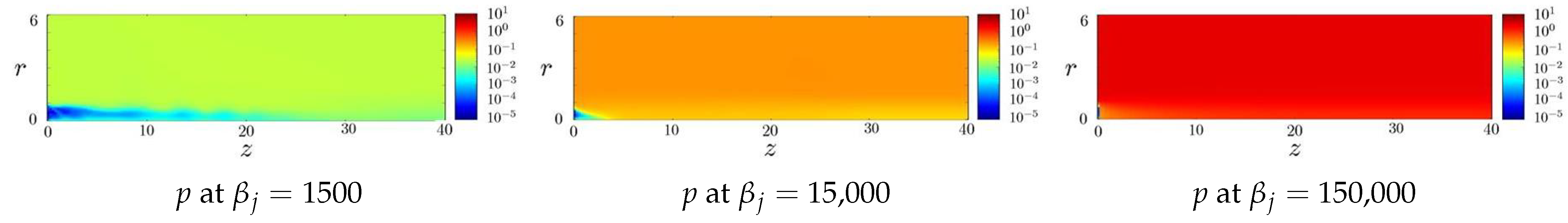
To study the effects of a strong magnetic field on the jet, the magnetization is increased to ${\beta }_j=$ 15,000 and 150,000 under a constant $\langle p_j\rangle$. The magnetic field strength is determined by the normalization factor $b_0$ on magnetic field, which is estimated by fitting the simulated synchrotron radiation to the observed data, which will be discussed in the next section.

The magnetic pitch angle is defined as

$$\begin{array}{ccc}& & {\varphi }_j={tan}^{-1}\frac{\langle B_{\varphi j}\rangle }{B_{zj}}\hfill \end{array}$$

(27)

In this work, we choose ${\varphi }_j=0^{\circ },{45}^{\circ }$ and 90${}^{\circ }$ to simulate the cases with poloidal, helical and toroidal magnetic field, respectively.

The jet structure is initially uniform in the z direction and is in equilibrium to the ambient medium. The jet pressure in the r direction is higher than the ambient pressure by an overpressure factor K [3], with $K=1.8$–2.5 [2,3,12]. In this work, we choose $K=2$. The overpressure of the jet causes periodic expansions and compressions in the z-direction, forming recollimation standing shocks.

The apparent speeds (${\beta }_a$) at different spots of the PKS 1502+106 were observed at 15, 43 and 86 GHz, which were used to estimate the viewing angle $\theta$ and injection speed $\beta$ [4]. In this work, the apparent speed is ${\beta }_a=7.1$, which was observed at 86 GHz [4]. The viewing angle and injection speed are estimated as

$$\begin{array}{ccc}& & \theta \simeq {\theta }_c^{\prime }={cos}^{-1}\frac{{\beta }_a}{\sqrt{1+{\beta }_a^2}}\simeq 8^{\circ }\hfill \end{array}$$

(28)

$$\begin{array}{ccc}& & \beta \simeq \frac{{\beta }_a}{\sqrt{1+{\beta }_a^2}}\simeq 0.99\hfill \end{array}$$

(29)

Note that apparent speed and variability Doppler factor were proposed in [4] to estimate the viewing angle. The apparent speed is chosen in this work.

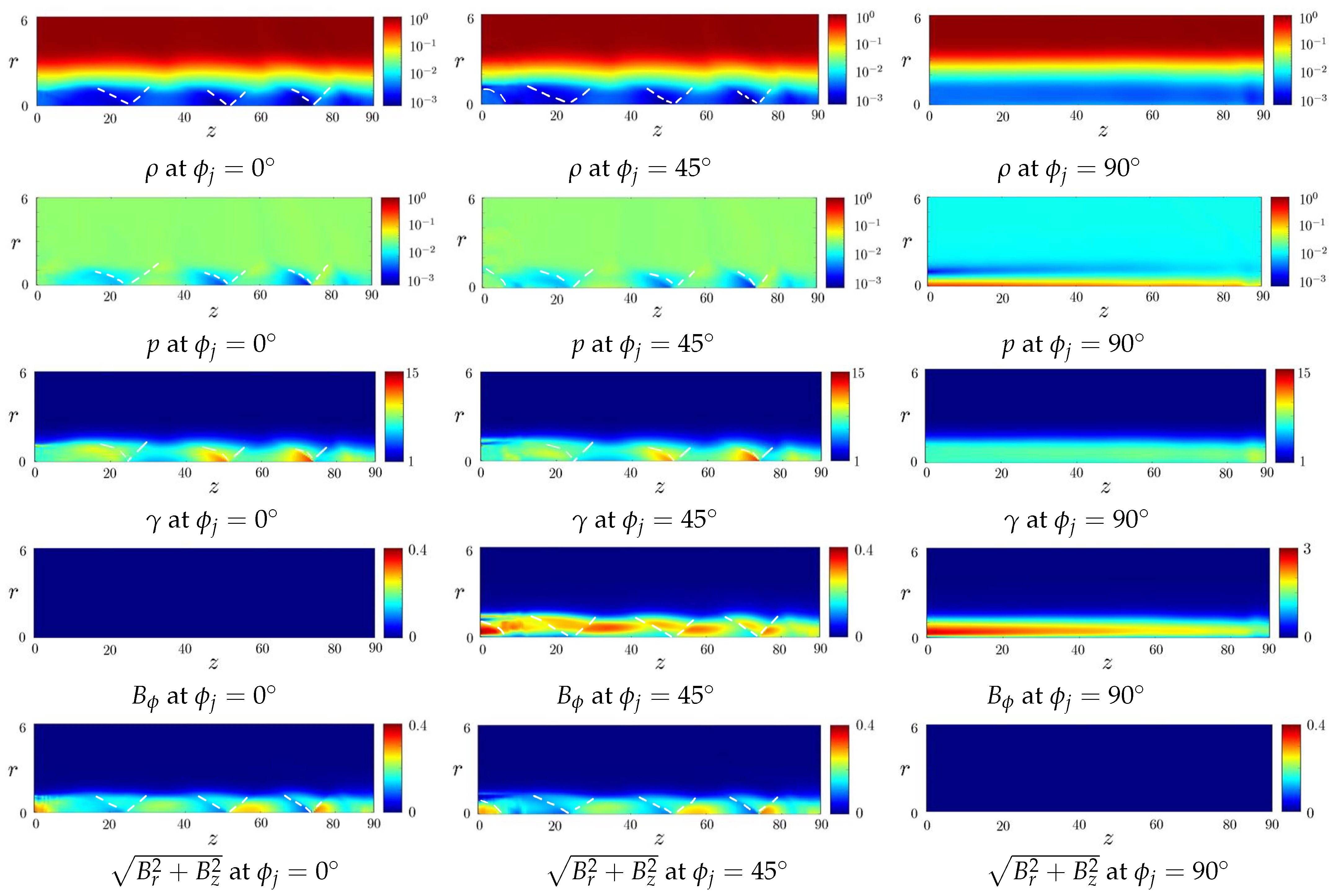
Figure 2 shows the effects of magnetic field morphology on the normalized plasma variables of jet models P1, HL1 and T1 with ${\beta }_j=1.5$. The mass density distributions in models P1 and HL1 are similar. Both P1 and HL1 models manifest alternate expansion and compression along the traveling direction. The recollimation standing shocks, which are marked by white dashed curves, are squeezed in the z-direction as the jet travels in the z-direction. The T1 model does not manifest recollimation standing shocks. The toroidal magnetic field induces a radial electric field $E_r=-B_{\varphi }\sqrt{1-1/{\gamma }^2}$, which confines the jet plasma in the spine region.

The gas pressure distributions in models P1 and HL1 manifest pitch patterns similar to their corresponding mass density distributions. The gas pressure distribution of the T1 model manifests a hot spine because the toroidal magnetic field confines most internal energy of the jet therein.

There is no toroidal magnetic field $B_{\varphi }$ in the P1 model. The toroidal magnetic field in the HL1 model manifests alternate expansion and compression in the z-direction along with the mass density and gas pressure, forming a plasmoid-like structure. The toroidal magnetic field in the T1 model does not display a periodic pattern, and its magnitude decreases in the z-direction due to dissipation of magnetic energy.

The poloidal magnetic field $\sqrt{B_r^2+B_z^2}$ in models P1 and HL1 manifests alternate expansion and compression in the z-direction, and there is no poloidal magnetic field in the T1 model.

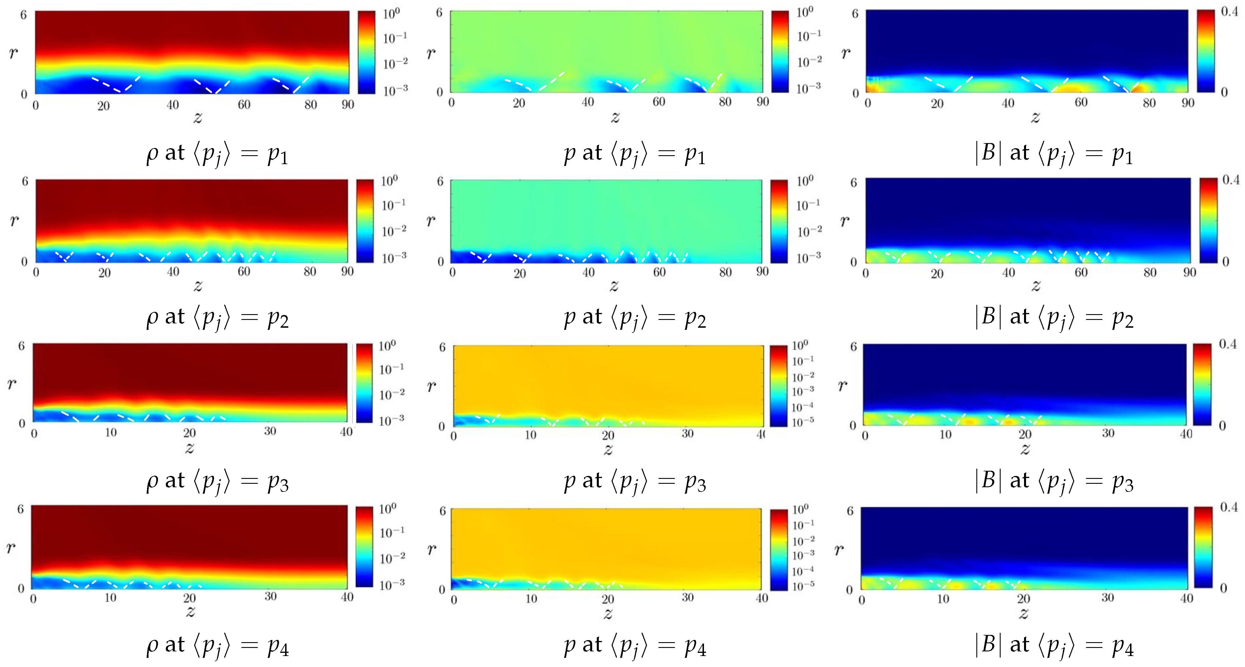
Figure 3 shows the effects of average gas pressure $\langle p_j\rangle$ on the normalized plasma variables of jets with a poloidal magnetic field, models P1, P2, P3 and P4, with the other parameters the same. In the P1 model, the mass density, gas pressure and magnetic field manifest alternate expansion and compression, forming recollimation standing shocks via overpressure and the Lorentz force exerted by the magnetic field. Four sets of expansion-and-compression patterns appear when $0\le z\le 90$, with the recollimation standing shocks marked by white dashed curves. Larger overpressure factor K leads to more significant expansion and compression [3]. The interval between two adjacent recollimation standing shocks becomes shorter when the jet travels away from the core.

In the P2 model, the recollimation standing shocks appear fainter than those in the P1 model. The fourth set of expansion-and-compression pattern extends to $z\simeq 45$. The intervals between adjacent recollimation standing shocks behind the fourth set become much shorter, and the recollimation standing shocks finally dissipate away. In the P3 model, the fourth set of the expansion-and-compression pattern extends to $z\simeq 22$, and the recollimation standing shocks beyond that dissipate away.

The results in models P1, P2 and P3 indicate that as the average gas pressure $\langle p_j\rangle$ becomes lower, the internal energy in the jet decreases, the expansion-and-compression pattern in the traveling direction becomes weaker and shorter.

In the P4 model, the fourth set of the expansion-and-compression pattern extends to $z\simeq 20$, and the patterns look similar to their counterparts in model P3, which implies the effect of $\langle p_j\rangle$ on the jet becomes insignificant when the internal energy in the jet is much smaller than that in the ambient plasmas.

Figure 4 shows the effects of magnetic field strength on the normalized plasma variables of the jets in models P4, P5 and P6, where $\langle p_j\rangle =3.31\times {10}^{-5}$. Equations (20) and (22) indicate that when $\langle p_j\rangle$ is fixed and $B_{zj}$ is increased, the gas pressure $p_a$ of ambient plasma is increased. In the P4 model, the gas pressure of ambient plasma is $p_a\simeq 0.024$, and the axial magnetic field is $B_{zj}\simeq 0.22$. The distribution of gas pressure displays 5 obscure periods of expansion and compression, and the jet reaches $z\simeq 22$.

In the P5 model, the gas pressure of ambient plasma is $p_a\simeq 0.24$, and the axial magnetic field is $B_{zj}\simeq 0.69$. The internal energy in the jet is not strong enough to overcome the Lorentz force exerted by the magnetic field to induce recollimation standing shocks. The jet reaches $z\simeq 4$, then dissipates in the ambient plasmas. In the P6 model, the gas pressure of ambient plasma is $p_a\simeq 2.5$, and the axial magnetic field is $B_{zj}\simeq 2.2$. The jet is immersed in the ambient plasmas at short distance from the core.

Figure 5 shows the effects of magnetic field morphology on the normalized plasma variables of the jets in models P4, HL2 and T2, where $\beta =1500$. The distributions of mass density and gas pressure in the P4 and HL2 models manifest similar expansion-and-compression patterns and recollimation standing shocks.

In the T2 model, the Lorentz force is not strong enough to pinch the jet, hence the overpressured jet expands radially to $r\simeq 5$. The distributions of mass density and gas pressure do not manifest expansion-and-compression patterns and recollimation standing shocks. The distributions of magnetic fields display similar features to their counterparts in Figure 2 with ${\beta }_j=1.5$. In the HL2 and T2 models, the initial gas pressure is set to $p=p_{min}={10}^{-6}$, and the gas pressure in equilibrium with the magnetic pressure is $p<p_{min}$.

In summary, the poloidal component of the magnetic field leads to alternate expansion-and-compression patterns, forming recollimation standing shocks, and the toroidal component of magnetic field confines the jet plasmas in the spine region and suppresses recollimation standing shocks. Lower average gas pressure $\langle p_j\rangle$ leads to less internal energy in the jet, the expansion-and-compression patterns become weaker and the period decreases. When the internal energy in the jet is much smaller than the ambient plasmas, the effects of $\langle p_j\rangle$ on the jets becomes insignificant. When the internal energy in the jet is not strong enough to overcome the Lorentz force, the jet dissipates over a short distance.

4. Synchrotron Radiation and Rotation Measure

Table 2. VLBI parameters for observing PKS 1502+106 [5,6].

Figure	Freq. (GHz)	Original Beam (mas × mas), PA	Restored Beam (mas × mas), PA	Contour of ${\mathit{I}}_{\mathit{b}}$ (mJy) per Beam	Contour of ${\mathit{I}}_{\mathit{\nu }}$ (erg/s/cm2/sr/Hz)
Figure 6a	1.64	$1510\times 1480$, 48.6${}^{\circ }$		$0.44\times (1,2,\cdots ,512)$	$7.4\times {10}^{-17}\times (1,2,\cdots ,512)$
Figure 6b	5	$79\times 49$, 24.4${}^{\circ }$		$3.0\times (1,2,\cdots ,1024)$	$4.3\times {10}^{-14}\times (1,2,\cdots ,1024)$
Figure 6c	2.3	$7.18\times 3.78$, $-{1.67}^{\circ }$	$7.18\times 3.78$, 0${}^{\circ }$	$3.5\times (1,2,\cdots ,256)$	$4.8\times {10}^{-11}\times (1,2,\cdots ,256)$

lists the parameters associated with Figure 6 in [5,6]. The original beam was used to measure the brightness $I_b$ (Jy/beam), which is related to the intensity $I_{\nu }$ (erg/s/cm${}^2$/sr/Hz), with the beam aperture of ${\Omega }_b$ (sr), as [5,6,24].

$$\begin{array}{ccc}& & I_{\nu }={10}^{23}\times I_b/{\Omega }_b\hfill \end{array}$$

(30)

The position angle (PA) is set to $0^{\circ }$ in the north direction, and increases towards the east direction.

Figure 6 shows the images of PKS 1502+106 observed in VLA, MERLIN and VLBA [5,6]. Figure 6a,b is transformed by using the original beams [5]; Figure 6c is transformed by using the restored beams.

The VLA image in Figure 6a was observed at 1.64 GHz. The jet segment manifests a low-brightness lobe, extending about $7^{″}$ (≃60 kpc) from the core to the southeast, at PA $={157}^{\circ }$. Note that the span of $1^{″}$ is equivalent to a projected distance of about $8.5$ kpc. The MERLIN image in Figure 6b was observed at 5 GHz. The jet segment extends about ${0.6}^{″}$ (≃5 kpc), at PA $\simeq {140}^{\circ }$. Four stationary knots, including the core, appear within the jet segment. The VLBA image in Figure 6c was observed at 2.3 GHz. The jet segment extends about 20 mas from the core, with PA $\simeq {80}^{\circ }$. In general, the intensity around the core of a jet segment is strong and becomes fainter away from the core.

Table 3. Parameters for simulating synchrotron radiation from PKS 1502+106.

Scale/Model	${\mathit{\psi }}^{\prime }$ (${}^{\circ }$)	${\mathit{L}}_{\mathbf{0}}$ (pc)	${\mathit{t}}_{\mathbf{0}}$ (s)	${\mathit{n}}_{\mathbf{0}}$ (1/cm3)	${\mathit{\rho }}_{\mathbf{0}}$ (g/cm3)	${\mathit{p}}_{\mathbf{0}}$ (dyn/cm2)	${\mathit{b}}_0$ (Gauss)
(b)/P1	230	340	$3.50\times {10}^{10}$	$1.85\times {10}^{-2}$	$1.68\times {10}^{-29}$	$1.52\times {10}^{-8}$	$4.36\times {10}^{-4}$
(b)/HL1	230	340	$3.50\times {10}^{10}$	$2.7\times {10}^{-3}$	$2.5\times {10}^{-30}$	$2.2\times {10}^{-9}$	$1.7\times {10}^{-4}$
(b)/T1	230	340	$3.50\times {10}^{10}$	$2.3\times {10}^{-4}$	$2.1\times {10}^{-30}$	$1.9\times {10}^{-10}$	$4.9\times {10}^{-5}$
(b)/P4	230	766	$7.88\times {10}^{10}$	$2.95\times {10}^{-1}$	$2.68\times {10}^{-28}$	$2.42\times {10}^{-7}$	$1.7\times {10}^{-3}$
(b)/HL2	230	766	$7.88\times {10}^{10}$	$1.65\times {10}^{-2}$	$1.5\times {10}^{-29}$	$1.35\times {10}^{-8}$	$4.12\times {10}^{-4}$
(b)/T2	230	766	$7.88\times {10}^{10}$	$1.85\times {10}^{-4}$	$1.68\times {10}^{-31}$	$1.52\times {10}^{-8}$	$4.36\times {10}^{-5}$
(a)/P4	255	11,200	$1.15\times {10}^{12}$	$1.33\times {10}^{-3}$	$1.21\times {10}^{-30}$	$1.09\times {10}^{-9}$	$1.17\times {10}^{-4}$
(a)/HL2	255	11,200	$1.15\times {10}^{12}$	$7.5\times {10}^{-5}$	$6.83\times {10}^{-32}$	$6.14\times {10}^{-11}$	$2.78\times {10}^{-5}$
(a)/T2	255	11,200	$1.15\times {10}^{12}$	$8.18\times {10}^{-7}$	$7.44\times {10}^{-34}$	$6.7\times {10}^{-13}$	$2.91\times {10}^{-6}$
(c)/HL2	171	18.5	$1.9\times {10}^9$	$1.56\times {10}^0$	$1.42\times {10}^{-27}$	$1.28\times {10}^{-6}$	$4\times {10}^{-3}$
(c)/T2	171	18.5	$1.9\times {10}^9$	$1.74\times {10}^{-2}$	$1.58\times {10}^{-29}$	$1.43\times {10}^{-8}$	$4.23\times {10}^{-4}$

${\psi }^{\prime }$: the angle between jet axis and −RA on celestial sphere (plane of sky).

lists the normalization factors and the angle ${\psi }^{\prime }$ between the projection of the jet and −RA for simulating the synchrotron radiation from different jet segments of different scales.

Referring to Figure 1, the projection length of the jet onto the plane-of-sky is $\ell ={\ell }_{0}sin\theta$. The angular separation in the observation image of the jet is ${\theta }_a=\ell /d_a={\ell }_{0}sin\theta /d_a$, where $d_a=d_{\ell }/{(1+z_r)}^2$ is the angular diameter distance, and $d_{\ell }$ is the luminosity distance [25]. The redshift of PKS 1502+106 is $z_r=1.8385$ [4]. By using the cosmological parameters $H_0=74$ km/s, ${\Omega }_m=0.27$ and ${\Omega }_{\Lambda }=0.73$ [4], the luminosity distance is $d_{\ell }=$ 14,176.8 Mpc. Then, the angular separation ${\theta }_a$ is used to determine ${\ell }_0$.

The normalization factor $L_0$ on length is chosen to match the length ${\ell }_0$ of the jet, and the normalization factor on time is set to $t_0=c/L_0$. The normalization factor $n_0$ is chosen by fitting the simulated intensity of synchrotron radiation with the observation data. Then, the other normalization factors are determined as ${\rho }_0=n_0{m}_0$, $p_0={\rho }_0{c}^2$ and $b_0=\sqrt{4\pi {\rho }_0{c}^2}$.

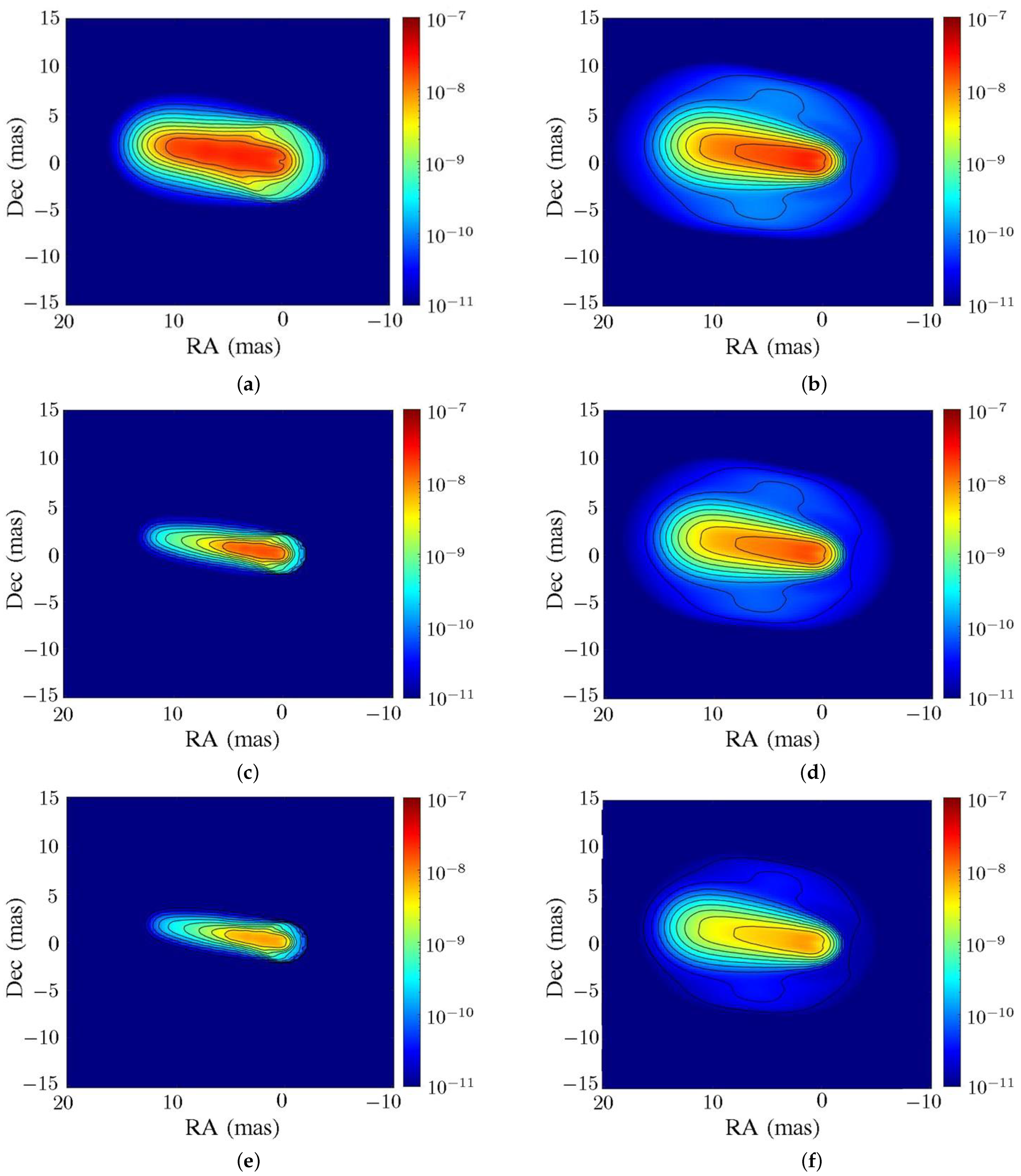
Figure 7 shows the effect of magnetic field morphology on the intensity of jet segments in scale b of models P1, HL1 and T1. The relativistic jet segment extends about ${0.5}^{″}$ to the southeast, with PA$={140}^{\circ }$. The intensity distribution in Figure 7a manifests four stationary knots, similar to Figure 6b. Figure 7b shows that the stationary knots in the intensity distribution become elongated and blurred as compared with those in the P1 model. The intensity distribution in Figure 7c shows no stationary knots, implying that the jet erupts from the core without recollimation. The toroidal magnetic field and the plasma flow induce a radial electric field $E_r$ to confine the jet; thus, most of the synchrotron radiation is emitted from the spine region.

Figure 8 shows the intensity distribution of jet segments (encircled with white contour) in scale b of models P4, HL2 and T2. Figure 8a shows that the structure of stationary knots and recollimation standing shocks are blurred and merged to a high-brightness region. The brightness of the jet decays in the z-direction, which is similar to the observation. The jet in Figure 8b is narrower than that in Figure 8a because the toroidal magnetic field component tends to confine the jet plasmas and smooth out the recollimation standing shocks. Figure 8c shows no stationary knots and the jet becomes wider in the transverse direction because the Lorentz force is not strong enough to balance the overpressure of the jet.

An electromagnetic wave propagating through a magnetized plasma experiences Faraday rotation. The total change of polarization angle due to Faraday rotation is given by [15]

$$\begin{array}{ccc}& & {\chi }_{\mathrm{obs}}-{\chi }_0=\frac{q_e^3{\lambda }^2}{2\pi m_0^2{c}^4}\int n\overline{B}·d\overline{\ell }=\mathrm{RM}{\lambda }^2\hfill \end{array}$$

(31)

where RM is the rotation measure, and ${\chi }_0$ and ${\chi }_{\mathrm{obs}}$ are the intrinsic polarization angle and the observed polarization angle, respectively, of the electric field. The RM value is typically estimated with multi-frequency observations, for example,

$$\begin{array}{ccc}& & \mathrm{RM}=\frac{{\chi }_{\mathrm{obs}1}-{\chi }_{\mathrm{obs}2}}{{\lambda }_1^2-{\lambda }_2^2}\hfill \end{array}$$

(32)

The observed polarization angles are derived from the Stokes parameters as in [26]

$$\begin{array}{ccc}& & {\chi }_{\mathrm{obs}1}=\frac{1}{2}\left[{tan}^{-1}\left(\frac{U_{\nu 1}}{I_{\nu 1}^{\left(a\right)}-I_{\nu 1}^{\left(b\right)}}\right)+m_1\pi \right],m_1=0,\pm 1,\pm 2\cdots \hfill \end{array}$$

(33)

$$\begin{array}{ccc}& & {\chi }_{\mathrm{obs}2}=\frac{1}{2}\left[{tan}^{-1}\left(\frac{U_{\nu 2}}{I_{\nu 2}^{\left(a\right)}-I_{\nu 2}^{\left(b\right)}}\right)+m_2\pi \right],m_2=0,\pm 1,\pm 2\cdots \hfill \end{array}$$

(34)

where $I_{\nu }^{\left(a\right)}$ and $I_{\nu }^{\left(b\right)}$ are the time-average intensities of two linearly polarized waves, $U_{\nu }=(I_{\nu }^{\left(a\right)}-I_{\nu }^{\left(b\right)})tan\left(2\chi \right)$, $\chi$ is the polarization angle and $m_1$ and $m_2$ are ambiguity numbers to account for phase wrapping.

By substituting (33) and (34) into (32), we have

$$\begin{array}{ccc}& & \mathrm{RM}=\frac{1}{2({\lambda }_1^2-{\lambda }_2^2)}\left[{tan}^{-1}\left(\frac{U_{\nu 1}}{I_{\nu 1}^{\left(a\right)}-I_{\nu 1}^{\left(b\right)}}\right)-{tan}^{-1}\left(\frac{U_{\nu 2}}{I_{\nu 2}^{\left(a\right)}-I_{\nu 2}^{\left(b\right)}}\right)\right]+\frac{\ell }{2({\lambda }_1^2-{\lambda }_2^2)}\pi \hfill \end{array}$$

(35)

where $\ell =m_1-m_2$.

Figure 9 shows the rotation measure (RM) distribution of jet segments in scale b, of models P4, HL2 and T2. Figure 9a shows the RM around the core at (RA, Dec) $=(0,0)$ in the P4 model is about $-3000$ (rad/m${}^2$). The RM drops to about $-6000$ (rad/m${}^2$) and then approaches 0 in the jet traveling direction; it increases to about $-2000$ (rad/m${}^2$) in the opposite direction. The magnitude of the RM in general decreases away from the spine of jet.

Figure 9b shows that the RM of the jet segment in the HL2 model is symmetrical about the jet axis and the magnitude of the RM is about 100 (rad/m${}^2$). The magnitude of the RM decreases to about 0 when the jet travels far away from the core. Figure 9c shows that the RM of the jet segment in the T2 model is symmetrical about the jet axis. The RM at the core is about $-0.008$ (rad/m${}^2$) and approaches 0 when the jet travels far away from the core.

Among these three models, the magnitude of the RM in the P4 model is the largest, and that of the T2 model is the smallest, being different by several orders of magnitude. The Faraday rotation, and hence the RM, are proportional to the parallel component of the magnetic field ($B_{\parallel }$). The PKS 1502+106 casts a small viewing angle $\theta$, the poloidal component of the magnetic field contributes large $B_{\parallel }$, leading to a large RM. On the other hand, the toroidal component of the magnetic field contributes small $B_{\parallel }$, leading to a small RM.

Figure 10 shows the Stokes parameters (erg/s/cm${}^2$/sr/Hz) computed along a LoS (s) path through (RA, Dec) $=(0,0)$ in scale b. Figure 10a shows that in the P4 model, the total intensity $I_{\nu }^{\left(a\right)}+I_{\nu }^{\left(b\right)}$ increases in $s<5$ (kpc), and remains almost constant beyond $s=5$ (kpc). The components $I_{\nu }^{\left(a\right)}$, $I_{\nu }^{\left(b\right)}$ and $U_{\nu }$ oscillate along s in $s<13$ (kpc) due to Faraday rotation.

Figure 10b shows that in the HL2 model, the total intensity increases when $s<5$ (kpc), and $I_{\nu }^{\left(a\right)}$ slightly decreases and $I_{\nu }^{\left(b\right)}$ slightly increases when $5<s<13$ (kpc). Figure 10c shows that in the T2 model, $I_{\nu }^{\left(a\right)}$, $I_{\nu }^{\left(b\right)}$ and their sum increase when $s<5$ (kpc), and remain almost unchanged beyond $s=5$ (kpc).

Figure 11 shows the synchrotron radiation intensity and RM of jet segments in scale a, of models P4, HL2 and T2. Figure 11a shows that the jet erupts from the origin with $I_{\nu }=7.6\times {10}^{-14}$ (erg/s/cm${}^2$/sr/Hz), and decreases in magnitude away from the core. Figure 11b shows similar features with that of the P4 model. The intensity of the jet segment in the HL2 model decreases faster than its counterpart in the P4 model away from the core. Figure 11c shows that the jet segment becomes wider in the transverse direction as the jet travels because the Lorentz force is not strong enough to confine the overpressure of the jet.

Figure 11d shows that the RM around the core is about $-15$ (rad/m${}^2$), and decreases to about $-30$ (rad/m${}^2$) when the jet travels to (RA, Dec) $=(1.2,-4.5)$ (${}^{″}$). The RM in the sheath region is smaller than that in the spine region. Figure 11e shows that the RM around the core is about $-0.2$ (rad/m${}^2$), and decreases to about $-0.4$ (rad/m${}^2$) when the jet travels to (RA, Dec) $=(1.2,-4.5)$ (${}^{″}$). Figure 11f shows that the RM around the core is about $-4\times {10}^{-5}$ (rad/m${}^2$) and quickly approaches 0 when the jet travels apart from the core. The magnitude of the RMin the P4 model is the largest, and that in the T2 model is the smallest.

By comparing Figure 9 and Figure 11, the magnitude of the RM in scale a is about three orders smaller than their counterpart in scale b. The Faraday rotation is proportional to the electron number density n and the parallel component of the magnetic field, $B_{\Vert }$. The product of normalization factors $n_0$ and $b_0$ in scale a is about three orders of magnitude smaller than that in scale a, which explains the order difference of the RM in Figure 9 and Figure 11.

Figure 12 shows the intensity of the jet segment in scale c of models HL2 and T2. The jet distribution when $0<r<6$ and $0<z<20$ is used to compute the synchrotron radiation, which is then compared with the observation data to confirm the morphology of the magnetic field in the PKS 1502+106.

Figure 12a shows that at $\nu =2.3$ GHz, the jet in the HL2 model erupts towards PA $={81}^{\circ }$, and the synchrotron radiation manifests slight compression and expansion. The magnitude of intensity is about $2.5\times {10}^{-8}$ (erg/s/cm${}^2$/sr/Hz). Figure 12b shows that at $\nu =2.3$ GHz, the jet in the T2 model expands in a radial direction because the Lorentz force is not strong enough to confine the jet. The synchrotron radiation does not manifest compression and expansion, and the magnitude of intensity is about $2.5\times {10}^{-8}$ (erg/s/cm${}^2$/sr/Hz).

Figure 12c–f shows the intensity maps at $\nu =4.6$ and 15.4 GHz. The radiation features are similar to those at $\nu =2.3$ GHz. At higher observation frequency, the intensity map narrows down to the spine region and the magnitude of intensity decreases.

In the P4 model of scale c, the strong poloidal magnetic field induces significant Faraday rotation, and the required spatial resolution along the LoS (s) path becomes so small that the integration of radiative transfer equations becomes unstable.

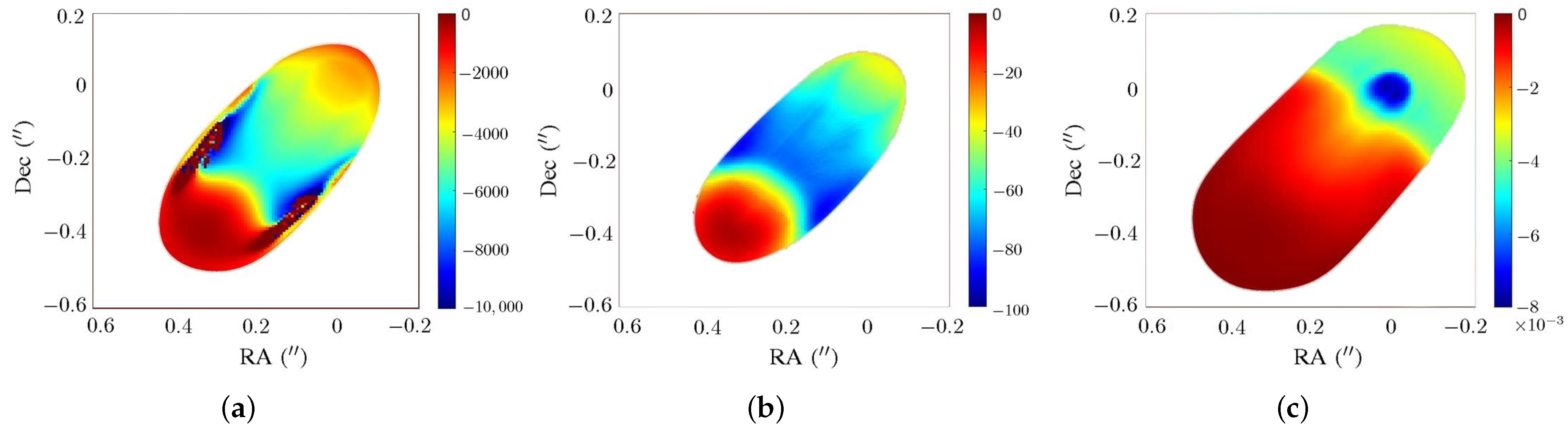
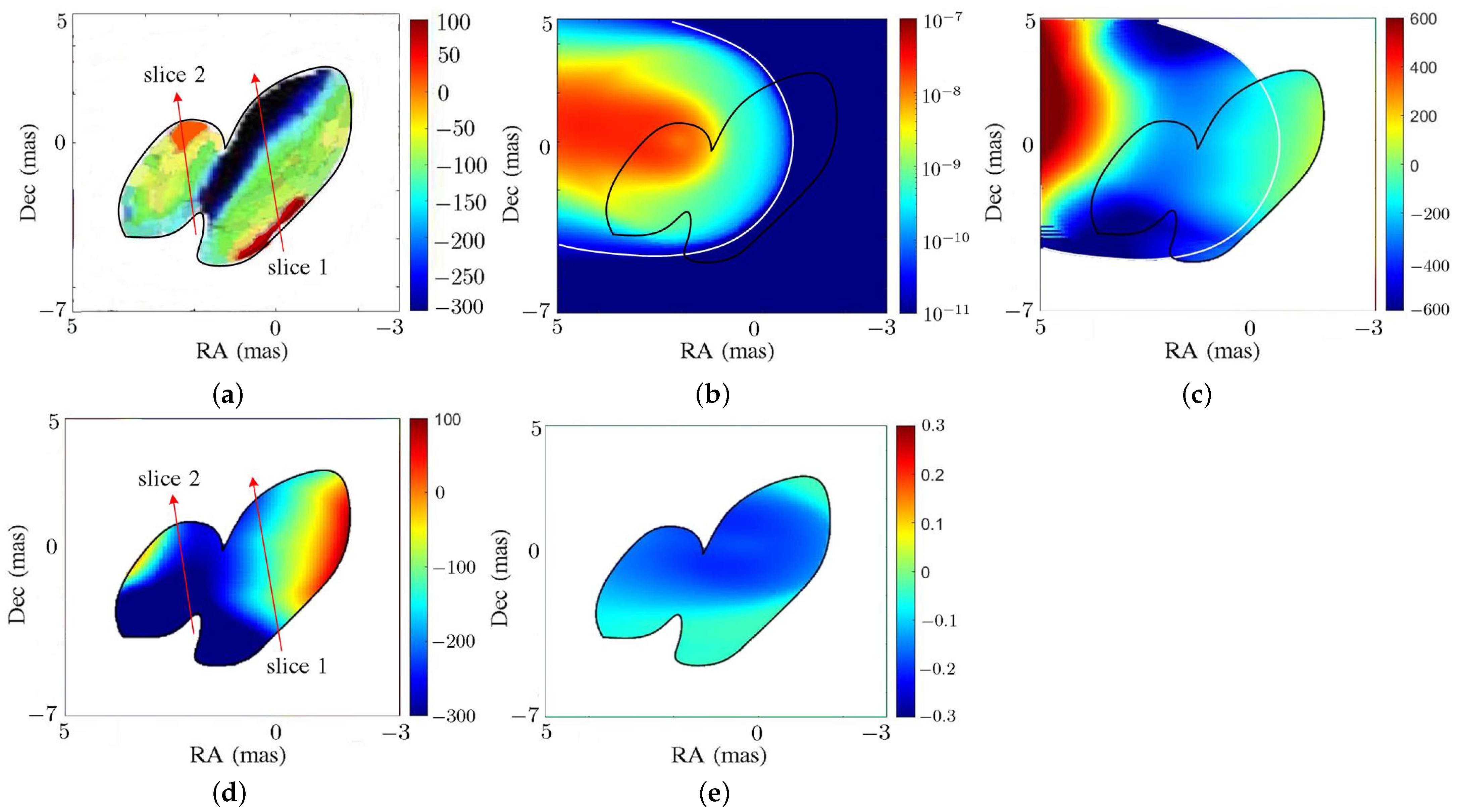
Figure 13 shows the comparison of the observed RM from the PKS 1502+106, in scale c, with the simulation results. Figure 13a shows the RM map of the PKS 1502+106 in the celestial sphere [7]. The RM around the core is about $-100$ (rad/m${}^2$), and decreases to about $-300$ (rad/m${}^2$) along the traveling direction of the jet. A strip with a positive RM of about 100 (rad/m${}^2$) appears around (RA, Dec) $=(0,-4)$ (mas), and another region with a positive RM of about 20 (rad/m${}^2$) appears around (RA, Dec) $=(2,0)$ (mas).

The RM map reveals a spine–sheath feature. The RM value changes from positive to negative along slice 1 across the core region, and from negative to positive along slice 2 across the side region. Slices 1 and 2 manifest a sign change and opposite RM gradients. All these features were conjectured to be related to either helical magnetic-field morphology or inhomogenous ambient medium [7,27,28]. Note that the RM was estimated with multi-frequency observations at 6 frequencies of 4.6, 5.0, 7.9, 8.9, 12.9 and 15.4 GHz [29].

Figure 13b shows the total intensity (erg/s/cm${}^2$/sr/Hz) from the PKS 1502+106. The jet region is encircled by a white contour and the observed region is encircled by a black contour. Figure 13c shows the RM by choosing the proper ambiguity integer ℓ. The RM around the core is about $-150$ (rad/m${}^2$), and decreases to about $-300$ (rad/m${}^2$) along the traveling direction of the jet. The RM increases to about 600 at RA $=5$ (mas) and decreases away from the spine of the jet.

Figure 13d shows that the RM map in the observed region manifests a positive RM of about 50 (rad/m${}^2$) in the west and decreases to $-300$ (rad/m${}^2$) towards the east. The RM oscillates along the traveling direction of the jet, manifesting a spine–sheath structure. The RM value changes from positive to negative along slice 1 across the core region; the RM value increases along slice 2 across the side region. Slices 1 and 2 reveal opposite RM gradients. The spine–sheath polarization structure, sign change in the RM slice and opposite RM gradients across the core and side regions are similar to the observation data.

Figure 13e shows the RM map in the T2 model, with $\nu =4.6$ and 15.4 GHz. The RM is negative and symmetrical about the jet axis. No alternate positive and negative regions are found. The magnitude of the RM is about 0.2 because the toroidal magnetic field contributes small $B_{\parallel }$. Both Faraday rotation and RM are proportional to the parallel component of magnetic field $B_{\parallel }$. The PKS 1502+106 casts a small viewing angle of $\theta =8^{\circ }$, the poloidal component of magnetic field contributes large $B_{\parallel }$ and the toroidal component of the magnetic field contributes small $B_{\parallel }$, hence the RM in the HL2 model is much larger than that in the T2 model.

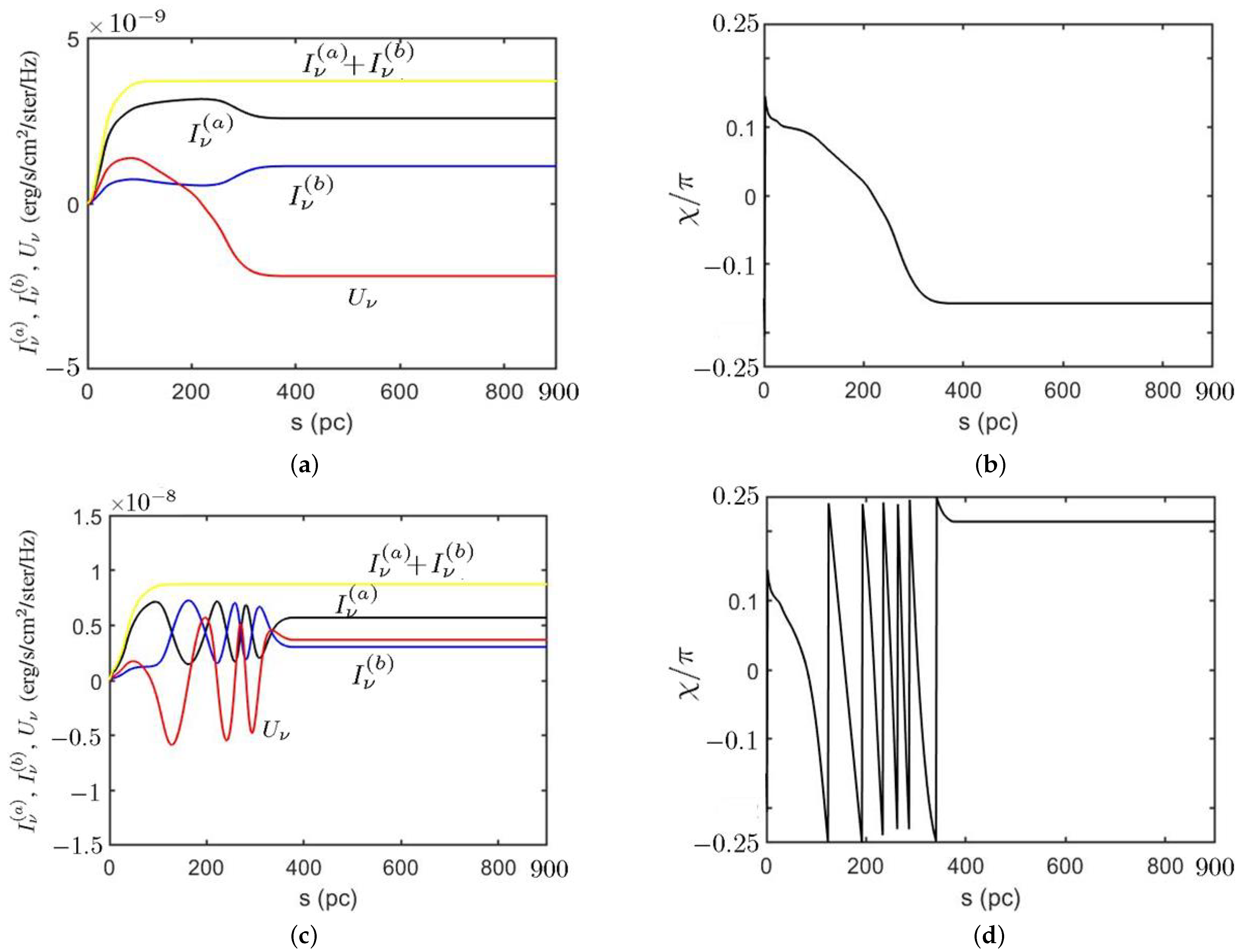
Figure 14 shows the Stokes parameters (erg/s/cm${}^2$/sr/Hz) and polarization angle (rad) of the HL2 model in scale c, computed at (RA, Dec) $=(0,0)$, with $\nu =4.6$ and $15.4$ GHz, respectively. The core of the jet is located at (RA, Dec) $=(0,0)$. Figure 14a shows that the emitting region lies in the range $0\le s\le 100$, and the magnitudes of $I_{\nu }^{\left(a\right)}$ and $I_{\nu }^{\left(b\right)}$ increase along s in the emitting region. Beyond $s=100$ (pc), the total intensity $I_{\nu }^{\left(a\right)}+I_{\nu }^{\left(b\right)}$ is almost unchanged, $I_{\nu }^{\left(a\right)}$ decreases and $I_{\nu }^{\left(b\right)}$ increases.

Figure 14b shows that the polarization angle decreases monotonically when $s<350$, in which the magnetic field induces Faraday rotation. Figure 14c shows that the emitting region lies in the range $0\le s\le 100$, and the total intensity $I_{\nu }^{\left(a\right)}+I_{\nu }^{\left(b\right)}$ is almost unchanged beyond $s=100$. The intensities $I_{\nu }^{\left(a\right)}$ and $I_{\nu }^{\left(b\right)}$ oscillate out of phase when $s<350$. The effect of Faraday rotation increases when the frequency decreases because $d{\chi }_F/ds\propto {\lambda }^2$. Figure 14d shows the polarization angle $\chi$ oscillates drastically between $-\pi /4$ and $\pi /4$ when $s<350$, which is consistent with the oscillation of the Stokes parameters.

5. Conclusions

A rigorous RMHD model has been developed to simulate the behaviors of the PKS 1502+106. The maps of synchrotron radiation intensity and rotation measure are also computed on the plane of sky, under different magnetic field morphologies. The simulation parameters are derived from the observation data of the PKS 1502+106. The effect of initial gas pressure, magnetic field strength and morphology on the jet have been simulated. The features under high magnetization ${\beta }_j$ and low gas pressure $\langle p\rangle$, compatible to the observation constraints on PKS 1502+106, have been specifically discussed. Recollimation standing shocks and plasmoid-like features in the toroidal magnetic field distribution are reproduced. The effects of magnetic field morphology and internal energy of jet on the synchrotron radiation maps are investigated. Conventional synchrotron radiation maps in the literature were computed without considering Faraday rotation. The simulated synchrotron radiation maps in different scales are compared to the observation data. The simulated intensity maps manifest similar size, shape and stationary knots as in the observation data. The simulated rotation measure maps manifest features of spine–sheath structure, sign change in the RM slice and opposite RM gradients by embedding a helical magnetic field in the jet. The simulated features in the rotation measure maps attest to the presence of a helical magnetic field as speculated in the literature.