Luenberger Position Observer Based on Deadbeat-Current Predictive Control for Sensorless PMSM

Abstract

Two problems can cause control performance degradation on permanent magnet synchronous motor (PMSM) systems, namely, fluctuation of PMSM parameters and the time delay between current sampling and command value update. In order to reduce the influence of these problems, a new current-predictive control strategy is proposed in this article for medium- and high-speed PMSM. This strategy is based on the discrete mathematical model of PMSM. This new control strategy consists of two main steps: First, an integrator is applied to calculate current compensation value; second, the predictive current value is obtained through deadbeat-current predictive method. The stability of predictive control system is also proved in the article. With this deadbeat-current predictive control scheme, the real current can reach the desired value within one control-step. Based on this new current control method, Luenberger observer and phase-locked loop position tracker is applied in this article. Experimental results for 0.4 kW surface-mounted PMSM confirm the validity and excellent performance for parameters fluctuation of new current predictive control.

1. Introduction

Nowadays, permanent magnet synchronous motors (PMSMs) have been widely used in industrial applications due to their high power and torque density, small size and wide-speed-range. In PMSM control system, the digital control is common applied for its high precision and excellent control performance. In particular, sensorless control and model predictive control are drawing increasing attention due to the concept of optimum control [1,2,3,4,5].

In sensorless control, position observer based on the voltage equations has been developed [6]. However, reliable operation of PMSM at high speeds still remains many challenges. For example, in medium- and high-speed, fundamental excitation model-based methods are applied to estimate position information [7,8,9,10,11,12,13,14,15,16,17]. Sliding model observer (SMO) is proposed in Reference [7] to estimate position, but signal chattering still exists in dynamic-state operation. A general phased-locked loop (PLL) position tracker is proposed to obtain position and speed information [8], but the gains in PLL are not easy to determine for its complex structure. A relationship between extended back electromotive force (extended back-EMF) and position error is built in [9], a model adaptive-reference system (MARS) is used in [10]. All of these methods are dependent on PMSM parameters excessively. A nonlinear observer [11,12] is presented to adapt nonlinear characteristic of PMSM, but the relationship between system stability and feedback gains is not clear and the robustness of observer cannot reach to desired performance. The method in [13] is based on cubature Kalman filter (CKF), which needs a large amount of calculation within one PWM control step, hence the method is difficult to realize in engineering. A Luenberger observer is built to observe position information in static-coordinate in References [14,15,16,17], which causes high phase-lag on estimated signal.

In current controller, model predictive control has been widely applied to achieve various functions, such as speed regulation [18], flux control [19], torque control [20] and current control [21,22,23,24,25,26,27]. In general, current control is divided into three parts: hysteresis control [21], proportional PI controller [22] and current predictive control [23,24,25,26,27]. In recent years, an increasing amount of attention has been drawn to current predictive control for its concept of optimum control. The calculation for command voltage value in controller needs a large amount of time, which causes time delay on command value updating, hence the aim of deadbeat predictive control is to predict the command value. Finally, the command value can follow desired current value in PMSM. Compared with conventional current predictive, deadbeat current control can catch command value within one control step under prediction principle [28]. However, the deadbeat-current predictive control is dependent on exact PMSM model, which means the mismatch of system parameters will cause the hysteresis between actual current and desired value [29]. In order to solve this problem, several methods are proposed [30,31,32]. In Reference [30], stator current error is reduced by using a current-regulated delta modulator with current error-correction. A robust current predictive control method [31] is proposed to reduce the current error, caused by inductance fluctuation, between measured error and desired command value. A method based on generalized nonlinear model [32] is presented to predict current, which shows excellent performance on reduce error in dynamic-state operation.

In this paper, a sensorless Luenberger position observer based on the proposed deadbeat-current predictive control is applied. Compared with aforementioned sensorless control methods, the method in this paper can decrease signal phase-lag and few fluctuations on model parameters will not produce the large position error, because a current compensation method is proposed to reduce current ripple. Moreover, the current value can catch current desired value within one PWM control period. The contribution of this article can be concluded as follows:

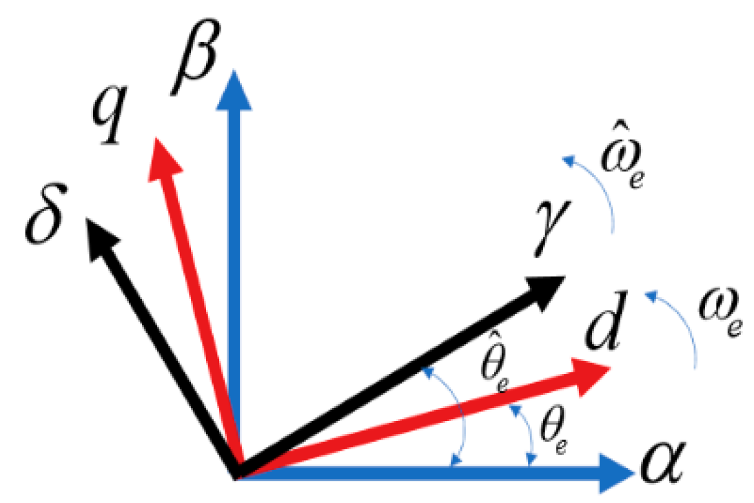
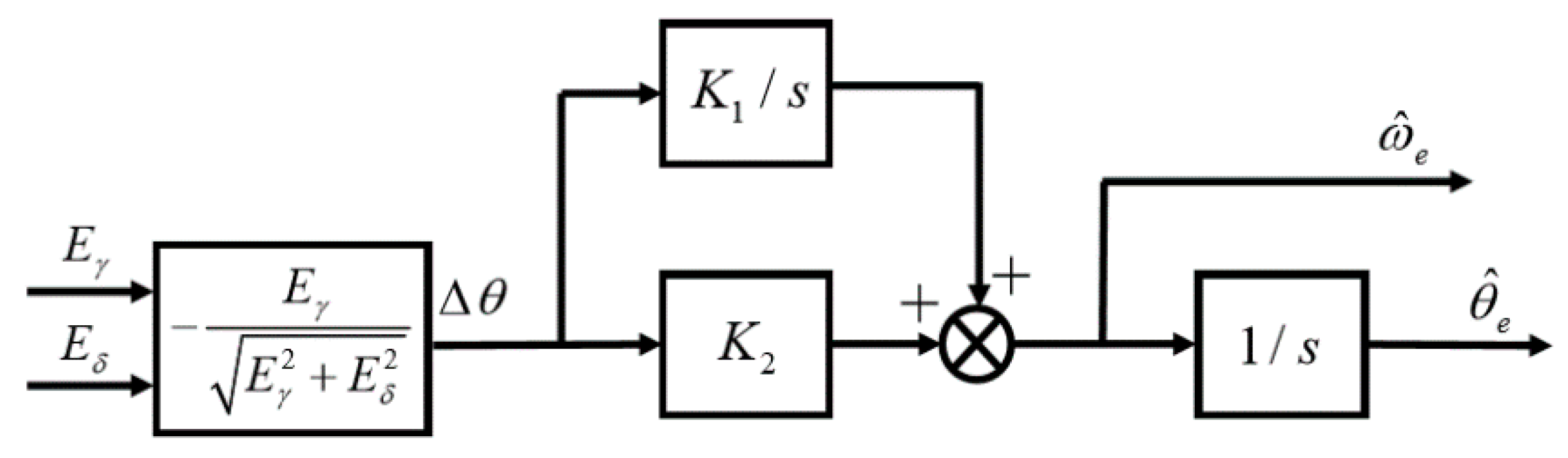
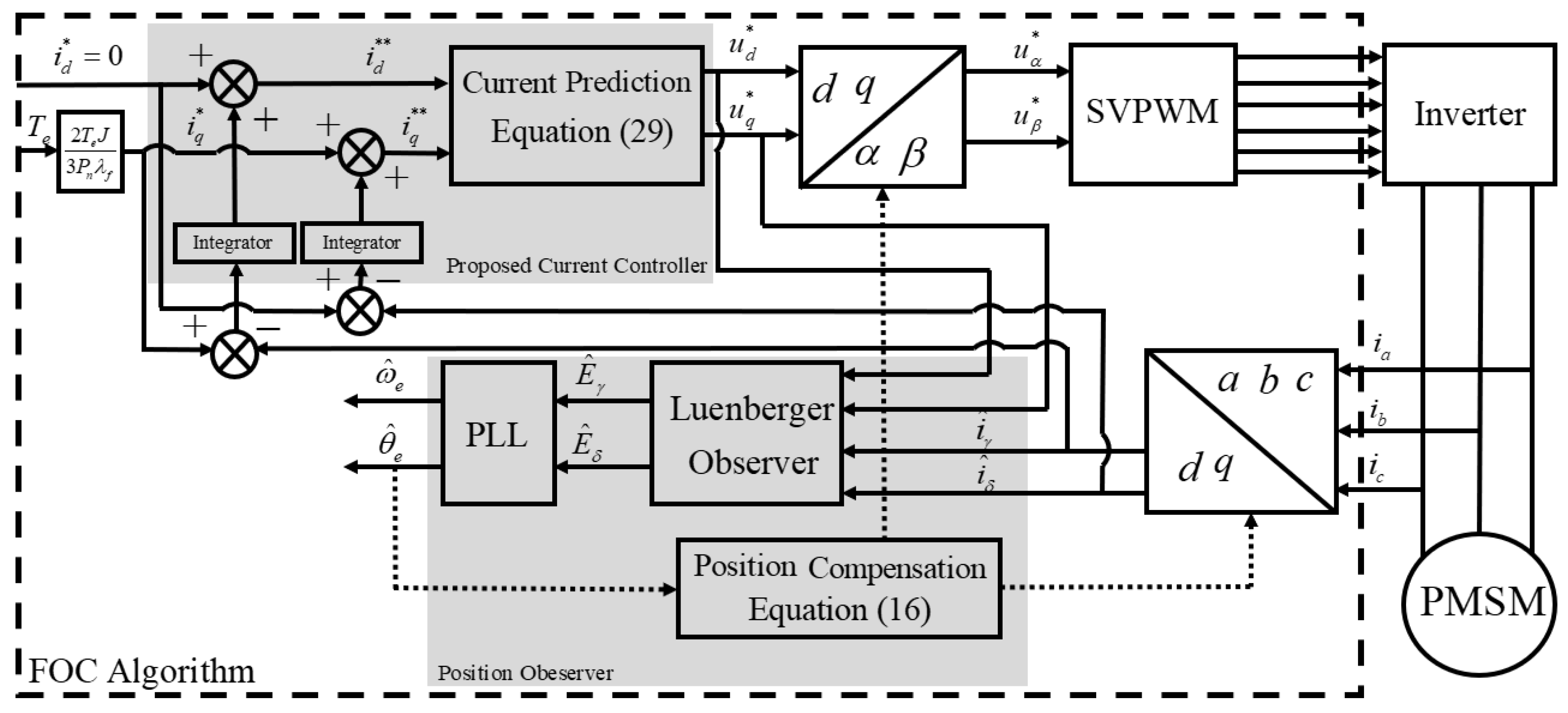
• In order to solve the phase-lag of estimated extended back-EMF, a Luenberger observer and two-order PLL position tracker are applied to observe the rotor position and speed.
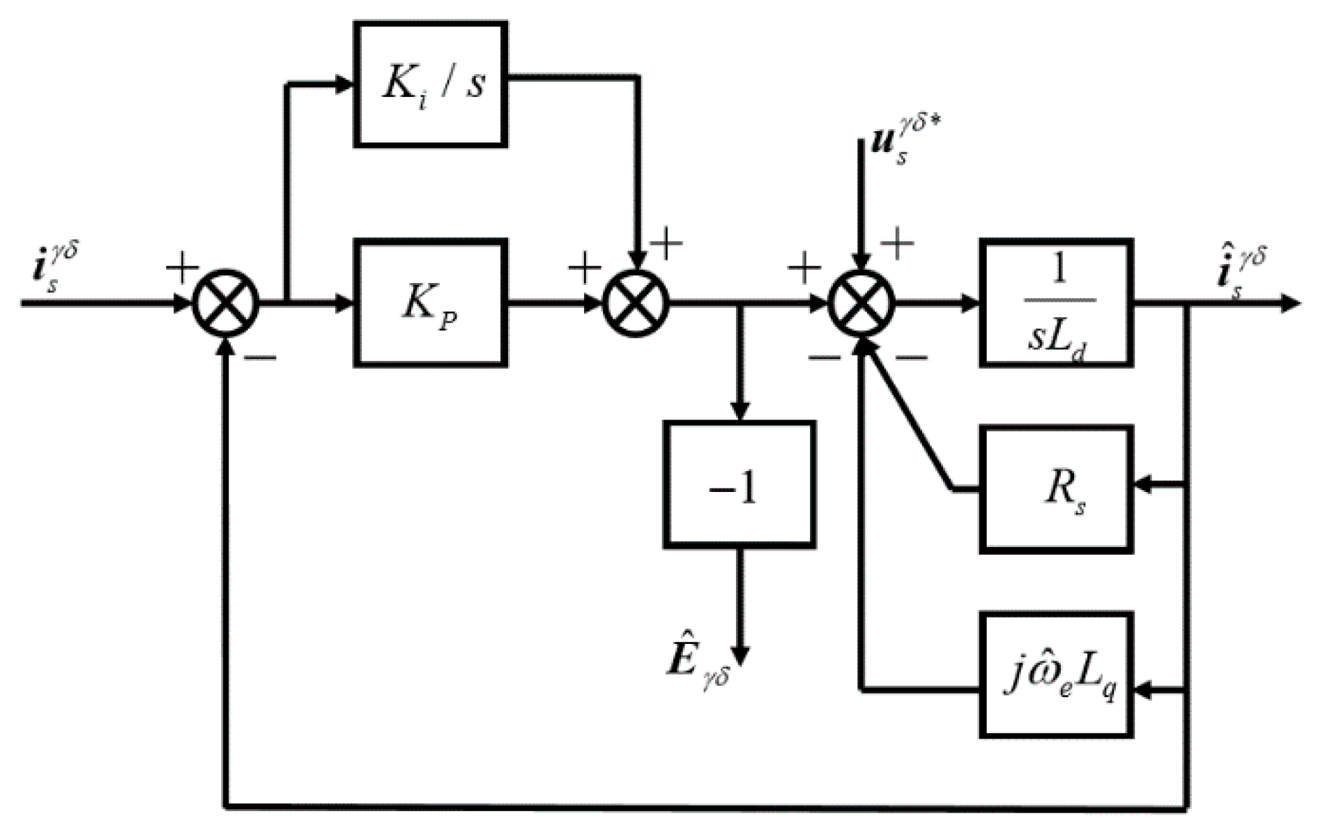
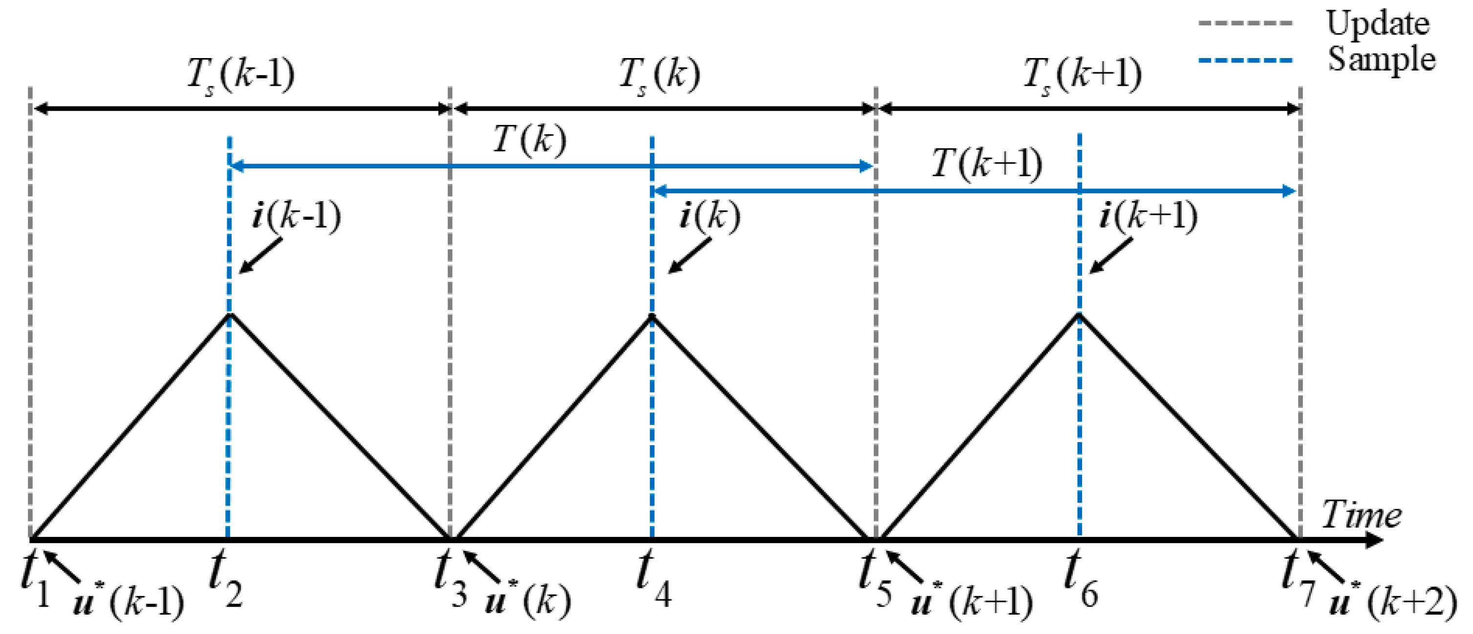
• Key PWM time-sequence logic relationship between current sampling and voltage command update is established. Based on this relationship, a deadbeat-current predictive method is proposed to calculate real-time voltage command value.
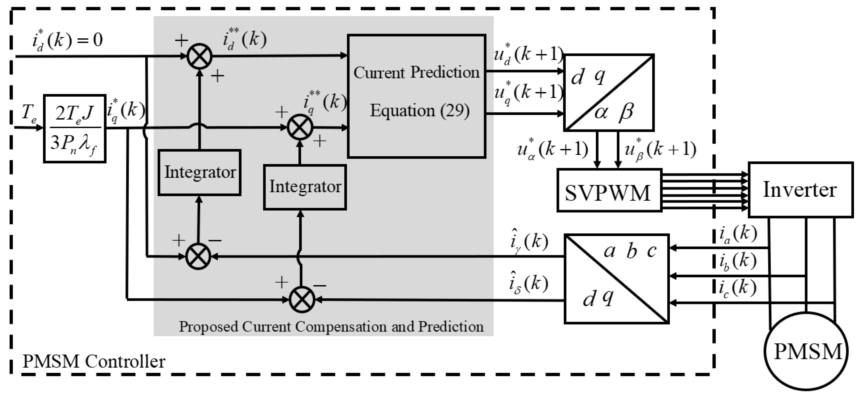
• Furthermore, due to the unavoidable parameter fluctuation of PMSM during operation, a current compensation method is proposed to reduce current ripple.

The rest of this paper is organized as follows: Section 2 establish the discrete mathematical model of PMSM and applies Luenberger observer to estimate rotor position; Section 3 presents current prediction model by analyzing PWM time-sequence logic and proposes a current compensation method; Section 4 conducts comparative experiments, which verify the validity of the whole control system; Finally, the conclusions of this article are listed in Section 5.

2. Rotor Speed and Position Observer

2.1. PMSM Mathematical Model

Due to the error between real rotor position and estimated rotor position, two reference rotational frames are considered. One is the real rotational coordinate system, which includes real rotor position ${\theta }_e$ and real rotor speed ${\omega }_e$, the other is the estimated rotational coordinate system, which includes estimated rotor position ${\widehat{\theta }}_e$ and estimated rotor speed ${\widehat{\omega }}_e$. Figure 1 shows two different rotating frames and one static frame. Then position error and speed error are defined as $\mathsf{\Delta }{\theta }_e$ and $\mathsf{\Delta }{\omega }_e$, respectively. Noticing that the real position and speed are unknown in operating control period, hence the PMSM model equations should be established in estimated rotor rotational frame. The voltage equation in d-q real rotational frame is established as follows:

$$\left(\begin{array}{c}{u}_d\\ u_q\end{array}\right)=\left(\begin{array}{cc}{R}_s+p{L}_d& -{\omega }_e{L}_q\\ {\omega }_e{L}_q& R_s+p{L}_d\end{array}\right)\left(\begin{array}{c}{i}_d\\ i_q\end{array}\right)+\left(\begin{array}{c}0\\ E_x\end{array}\right)$$

(1)

where $u_d$ and $u_q$ are stator voltage components in actual rotational frame, $i_d$ and $i_q$ are stator current components in actual rotational frame, $R_s$ is the stator resistance, $L_d$ and $L_q$ are the d- and q-axis inductances, respectively. $E_x={\omega }_e{\lambda }_f-p(L_d-L_q)i_q+{\omega }_e(L_d-L_q)i_d$ is extended back-EMF, ${\lambda }_f$ is permanent magnet (PM) flux and p is a differential operator $d/dt$.

For the convenience of analysis, using complex vector to transfer Equation (1) into:

$$u_s^{dq}=R_s{i}_s^{dq}+L_{d}p{i}_s^{dq}+j{\omega }_e{L}_q{i}_s^{dq}+j{E}_{ex}$$

(2)

where $u_s^{dq}=u_d+j{u}_q$ and $i_s^{dq}=i_d+j{i}_q$ are the stator voltage and current vectors.

Considering the position error, the sampling current can be transferred into estimated rotational frame by using estimated position vector operator (Equation (3)) for the actual position is unknown.

$$u_s^{dq}=u_s^{\gamma \delta }{e}^{-j\mathsf{\Delta }\theta },i_s^{dq}=i_s^{\gamma \delta }{e}^{-j\mathsf{\Delta }\theta }$$

(3)

Submitting the vector operator Equation (3) into Equation (2), the PMSM model in the ($\gamma -\delta$) estimated rotor reference frame is obtained, where the stator voltage equation is shown as follows:

$$u_s^{\gamma \delta }=R_s{i}_s^{\gamma \delta }+L_d\left(p{i}_s^{\gamma \delta }\right)-j{L}_d{i}_s^{\gamma \delta }\left(p\mathsf{\Delta }\theta \right)+j{\omega }_e{L}_q{i}_s^{\gamma \delta }+j{E}_{ex}{e}^{j\mathsf{\Delta }\theta }$$

(4)

In this article, the aim of Luenberger observer is to obtain extended back-EMF. Since the sampling current in rotational frame satisfies the Equation (4), hence the Equation (4) is set as reference model of current observer. Ignoring the parameters fluctuation in PMSM, using command voltage value $u_s^{\gamma \delta *}$ to replace actual voltage value $u_s^{\gamma \delta }$ in estimated frame. Considering the speed error keep in steady-state operation is zero ($d\mathsf{\Delta }\theta /dt=\mathsf{\Delta }\omega =0$), the reference PMSM model Equation (4) can be rewritten as:

$$\frac{d{i}_s^{\gamma \delta }}{dt}=\frac{1}{L_d}\left(u_s^{\gamma \delta *}-R_s{i}_s^{\gamma \delta }-j{\omega }_e{L}_q{i}_s^{\gamma \delta }-j{E}_{ex}{e}^{j\mathsf{\Delta }\theta }\right)$$

(5)

Based on reference model Equation (5), the current observer equation is designed as:

$$\frac{d{\widehat{i}}_s^{\gamma \delta }}{dt}=\frac{1}{L_d}\left(u_s^{\gamma \delta *}-R_s{\widehat{i}}_s^{\gamma \delta }-j{\widehat{\omega }}_e{L}_q{\widehat{i}}_s^{\gamma \delta }-j{\widehat{E}}_{ex}{e}^{j\mathsf{\Delta }{\theta }_e}\right)$$

(6)

Subtracting Equation (6) from Equation (5), defining the current error as $\mathsf{\Delta }{i}_s^{\gamma \delta }=i_s^{\gamma \delta }-{\widehat{i}}_s^{\gamma \delta }$. Since the current components in rotational frame is direct current (DC), the result is deduced as:

$$-\mathsf{\Delta }{i}_s^{\gamma \delta }\left(R_s+j{\widehat{\omega }}_e{L}_q\right)=L_d\left(E_{\gamma \delta }-{\widehat{E}}_{\gamma \delta }\right)$$

(7)

Apparently, estimated extended back-EMF is related to current error, hence the amplitude of estimated extended back-EMF can be adjusted by current error, the adjustment strategy is given by:

$$-{\widehat{E}}_{\gamma \delta }=\mathsf{\Delta }{i}_s^{\gamma \delta }\left(K_P+\frac{K_i}{s}\right)$$

(8)

In order to analysis the frequency characteristic of observer system, submitting Equation (8) into Equation (6), and using Laplace transform to figure out the relationship between $E_{\gamma \delta }$ and ${\widehat{E}}_{\gamma \delta }$, the relationship is described as:

$${\widehat{E}}_{\gamma \delta }=\frac{K_{P}s+K_i}{L_d{s}^2+(K_p+R_s)s+K_i}{E}_{\gamma \delta }$$

(9)

Noting that the observer is a second-order system, which produces hysteresis on high-frequency signal above cut-off frequency. Nevertheless, the estimated variate in rotational frame is a direct signal ${\widehat{E}}_{\gamma \delta }$, hence the hysteresis of the second-order system makes no difference on $E_{\gamma \delta }$. In conclusion, the structure of extended back-EMF Luenberger observer is shown in Figure 2.

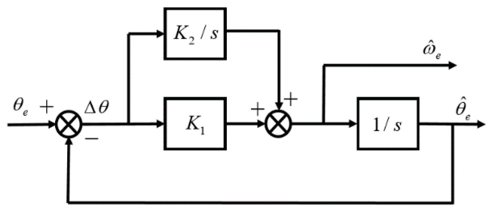
2.2. Second-Order PLL Rotor Position Tracker

In this article, PLL is applied to obtain the rotor position information from estimated extended back-EMF. Writing the vector ${\widehat{E}}_{\gamma \delta }$ into matrix form as follows:

$${\widehat{E}}_{\gamma \delta }=j{E}_{ex}{e}^{j\mathsf{\Delta }\theta }=\left(\begin{array}{l}{E}_{\gamma }\\ E_{\delta }\end{array}\right)=E_{ex}\left(\begin{array}{l}-\sin \mathsf{\Delta }\theta \\ \cos \mathsf{\Delta }\theta \end{array}\right)$$

(10)

In proposed method, the input of PLL is position error $\mathsf{\Delta }\theta$, which can be calculated by following equation under the assumption of $\sin \mathsf{\Delta }\theta \approx \mathsf{\Delta }\theta$:

$$\mathsf{\Delta }\theta \approx -\frac{E_{\gamma }}{\sqrt{E_{\gamma }^2+E_{\delta }^2}}$$

(11)

After determining system input, a position tracker structure is designed in Figure 3.

In order to determine the gains $K_1$ and $K_2$, the system is equivalent simplified to a second-order system, which is shown in Figure 4.

Hence the transfer function can be described by:

$$G(s)=\frac{{\widehat{\theta }}_e(s)}{{\theta }_e(s)}=\frac{K_{1}s+K_2}{s^2+K_{1}s+K_2}$$

(12)

The parameters $K_1$ and $K_2$ of PI (Proportional-Integral) controller are determined by choosing the damping rati $\varsigma =0.707$. In the meanwhile, the estimated error of the system is calculated by Equation (13)

$$E(s)=\mathsf{\Delta }\theta (s)={\theta }_e\left[1-G(s)\right]$$

(13)

The rotor speed in a steady-states is a constant, the rotor position is regarded as a ramp signal, whose Laplace form is ${\theta }_e(s)={\omega }_e/s^2$. By using final value theorem, the accuracy of the PLL position tracker can be judged by:

$$E(\infty )=\underset{s\to 0}{\lim }s\times \mathsf{\Delta }\theta (s)=\underset{s\to 0}{\lim }s\times \frac{{\omega }_e}{s^2}\left(1-\frac{K_{1}s+K_2}{s^2+K_{1}s+K_2}\right)=0$$

(14)

Obviously, the result shows high reliability of PLL position tracker.

In actual control process, the sampling current is discrete signal. An essential issue should be considered in discrete model, which is that the estimated speed information ${\widehat{\omega }}_e$ and operator $e^{j{\widehat{\theta }}_e}$ are unknown during operation. In order to obtain ${\widehat{\omega }}_e$ and $e^{j{\widehat{\theta }}_e}$ in operation period, the ${\widehat{\omega }}_e$ and ${\widehat{\theta }}_e$ in operation PWM period should be calculated by last period. The compensation strategy is designed as:

$${\widehat{\theta }}_{\mathrm{e}}(k)={\widehat{\theta }}_{\mathrm{e}}(k-1)+{\widehat{\omega }}_e(k-1)\times T_s$$

(15)

$${\widehat{\omega }}_{\mathrm{e}}(k)={\widehat{\omega }}_e(k-1)$$

(16)

where k is the number of control period and $T_s$ is the time of one control period.

3. Proposed and Conventional Current Prediction Model

In order to realize optimum control on PMSM, the concept of current prediction was referred to track real-time command current value for several years. On the other hand, the input of observer is command voltage value and current value. In order to guarantee the accuracy of observer input, the deadbeat-current predictive control is used. The fundament of current predictive control is discrete model of PMSM. In this article, Forward Euler method is applied to discretize model Equation (1), the discrete mathematical model of PMSM can be deduced as:

$$i(k+1)=F(k)\times i(k)+G\times u(k)+H(k)$$

(17)

where, $i(k+1)$ and $i(k)$ are discrete current vectors, $i(k+1)=\left(\begin{array}{c}{i}_d(k+1)\\ i_q(k+1)\end{array}\right)$, $i(k)=\left(\begin{array}{c}{i}_d(k)\\ i_q(k)\end{array}\right)$; $u(k)$ is discrete voltage vector $u(k)=\left(\begin{array}{c}{u}_d(k)\\ u_q(k)\end{array}\right)$; $F(k)=\left(\begin{array}{cc}1-\frac{T_s{R}_s}{L_d}& \frac{T_s{L}_q{\omega }_e(k)}{L_d}\\ -\frac{T_s{L}_d{\omega }_e(k)}{L_q}& 1-\frac{T_s{R}_s}{L_q}\end{array}\right)$; $H(k)=\left(\begin{array}{c}0\\ -\frac{{\lambda }_f{T}_s{\omega }_e(k)}{L_q}\end{array}\right)$;

$G=\left(\begin{array}{cc}\frac{T_s}{L_d}& 0\\ 0& \frac{T_s}{L_q}\end{array}\right)$.

3.1. Conventional Current Predictive Model

In actual computer control system, the command voltage in current time cannot be applied in operating control period. Therefore, the command value in next control period should be predicted in running control period. Equation (17) can be extended to next control period:

$$i(k+2)=F(k+1)\times i(k+1)+G\times u(k+1)+H(k+1)$$

(18)

An assumption is set to be a precondition, which means that the command current value in operating control period can track the command current in control period after next with deadbeat. The relationship can be written as:

$$i^{*}(k)=i^{*}(k+2)$$

(19)

Submitting Equation (19) into Equation (17) and Equation (18), the conventional current predictive model is obtained as:

$$u^{*}(k+1)=G^{-1}\left\{i^{*}(k)-F(k+1)\times \left[F(k)\times i(k)+Gu(k)+H(k)\right]-H(k+1)\right\}$$

(20)

The conventional current predictive method neglects the fluctuation of current value within predictive period, which influences the predictive control performance. Hence, a new predictive control method is proposed in this article.

3.2. Deadbeat Linearized Current Predictive Model

Considering the influence of PWM time-sequence on predictive period, the logic of PWM sampling time point and value updating time point are necessary to be analyzed. The relationship between sampling time point and command updating time point is shown in Figure 5.

Noticing that the sampling time point is the midpoint of per PWM control period, the voltage updating time point is the beginning of every period. According to the closed-loop control strategy of PMSM, the voltage command value is calculated by a controller whose input is current command value. The sampling current $i(k-1)$ and are used to predict voltage command value $u^{*}(k+1),u^{*}(k+2)$, respectively, hence the predictive period $T=1.5T_s$ The predictive period is longer than the control period, which means that the actual current cannot reach to desired command value within one PWM control period based on conventional predictive method.

Since the sampling time is usually short, the fluctuation of rotor speed tends to be zero and the change of current within one PWM period is approximated to linear. Moreover, the average voltage value within half of a PWM control period is voltage value in running PWM control period. For instance, the average voltage value in half of period $[t_1,t_2]$ or $[t_2,t_3]$ is $u^{*}(k-1)$ in Figure 5. Considering this condition, the voltage can be integrated within one predictive period as following equations:

$$\{\begin{array}{l}{\displaystyle {\int }_t^{1.5T_s+t}{u}_{d}dt}=\frac{u_d^{*}(k)+2u_d^{*}(k+1)}{2}\times T_s\\ {\displaystyle {\int }_t^{1.5T_s+t}{u}_{q}dt}=\frac{u_q^{*}(k)+2u_q^{*}(k+1)}{2}\times T_s\\ {\displaystyle {\int }_t^{1.5T_s+t}{i}_{q}dt}=\frac{i_q^{*}(k)+i_q^{*}(k+1)}{2}\times 1.5T_s\end{array}$$

(21)

The current command value in next period cannot be obtained in running PWM control period, therefore the command value in running PWM control period is used to replace the unknown value. Submitting Equation (21) into Equation (1), the current predictive model is obtained as:

$$\{\begin{array}{l}\frac{u_d^{*}(k)+2u_d^{*}(k+1)}{3}=R_s\frac{i_d(k)+i_d^{*}(k)}{2}+L_d\frac{2\left(i_d^{*}(k)-i_d(k)\right)}{3}-{\omega }_e(k)L_q\frac{i_q(k)+i_q^{*}(k)}{2}\\ \frac{u_q^{*}(k)+2u_q^{*}(k+1)}{3}=R_s\frac{i_q(k)+i_q^{*}(k)}{2}+L_q\frac{2\left(i_q^{*}(k)-i_q(k)\right)}{3}-{\omega }_e(k)L_d\frac{i_d(k)+i_d^{*}(k)}{2}+{\omega }_e(k){\lambda }_f\end{array}$$

(22)

Compared with conventional predictive control method, the method presented in this paper considers the PWM time-sequence with linear current prediction, which improves the performance on tracking current and realizes deadbeat control.

3.3. Current Compensation

The aim of current compensation is to improve the disturbance rejection behavior. In this article, the vector control strategy is based on $i_d^{*}=0$, therefore only the $i_q$ current predictive model in Equation (22) should be considered. Equation (22) can be rewritten as:

$$\frac{u_q^{*}(k)+2u_q^{*}(k+1)}{3}=R_s\frac{i_q(k)+i_q^{*}(k)}{2}+L_q\frac{2\left(i_q^{*}(k)-i_q(k)\right)}{3T_s}+{\omega }_e(k){\lambda }_f$$

(23)

Equations (22) and (23) are the most important equations in this article. Ideally, the current in next PWM control period can catch the current command value $i_q^{*}$. However, in actual case the parameters fluctuation of PMSM are not sufficiently small to be ignored, hence the disturbance factors should be analyzed. Equation (23) is established as the ideal model of voltage control, the actual voltage control model is established as Equation (24), which includes actual parameters of PMSM in running time:

$$\frac{u_q^{*}(k)+2u_q^{*}(k+1)}{3}=R_s^{\prime }\frac{i_q(k)+i_q(k+1)}{2}+L_q^{\prime }\frac{2\left(i_q(k+1)-i_q(k)\right)}{3T_s}+{\omega }_e(k){\lambda }_f^{\prime }$$

(24)

where $R_s^{\prime }$, $L_q^{\prime }$, ${\lambda }_f^{\prime }$ are actual stator resistance, inductance in q-axis and PM flux, respectively.

In order to explore the relationship between parameters fluctuation and current error, subtract Equation (23) from Equation (24) and the result is:

$$i_q(k+1)=\frac{(-3\mathsf{\Delta }{R}_s{T}_s+4\mathsf{\Delta }{L}_q)i_q(k)+(3R_s{T}_s+4L_q)i_q^{*}(k)}{3R_s^{\prime }{T}_s+4L_q^{\prime }}+\frac{{\omega }_e(k)\mathsf{\Delta }{\lambda }_f}{3R_s^{\prime }{T}_s+4L_q^{\prime }}=i_{q1}(k+1)+i_{q2}(k+1)$$

(25)

where $\mathsf{\Delta }{R}_s=R_s^{\prime }-R_s$, $\mathsf{\Delta }{L}_q=L_q^{\prime }-L_q$, $\mathsf{\Delta }{\lambda }_f={\lambda }_f^{\prime }-{\lambda }_f$, $i_{q1}(k+1)$ includes the disturbance produced by $\mathsf{\Delta }{R}_s$ and $\mathsf{\Delta }{L}_q$, $i_{q2}(k+1)$ includes the disturbance produced by $\mathsf{\Delta }{\lambda }_f$.

Noticing that $T_s$ is sufficient small, hence one inequation relationship can be established: $\left|3R_s{T}_s\right|\ll \left|4L_q\right|$. Based on this relationship, Equation (25) is simplified as:

$$i_q(k+1)=\frac{\mathsf{\Delta }{L}_q{i}_q(k)+L_q{i}_q^{*}(k)}{L_q^{\prime }}$$

(26)

The transfer function in discrete form of Equation (26) is described by:

$$\frac{i_q(z)}{i_q^{*}(z)}=\frac{L_q/L_q^{\prime }}{z+(L_q/L_q^{\prime })-1}$$

(27)

Equation (27) indicates that the current can follow the command value within one PWM control period when $L_q/L_q^{\prime }=1$.

Considering more interference factors, the sakes for current error are not limited by parameters fluctuation. Low-order harmonics produced by SVPWM, dead-time and voltage drop of inverter, bus voltage ripple and measurement noise of system can also cause current error. In order to reduce current error, all of the above interference factors in operation control period are regarded as one disturbing term. Considering $f_q(k)$, the predictive current in q-axis consists of 3 parts, which is described as:

$$i_q(k+1)=\frac{\mathsf{\Delta }{L}_q{i}_q(k)+L_q{i}_q^{*}(k)}{L_q^{\prime }}+\frac{{\omega }_e(k)\mathsf{\Delta }{\lambda }_f}{3R_s^{\prime }{T}_s+4L_q^{\prime }}+f_q(k)$$

(28)

According to Equation (28), this article presents a compensation method by using integrator to obtain the compensation value $i_q^{**}(k)$. Adding the compensation value to current command value, the compensated value can be applied to predict voltage command.

Using new current command value $i_q^{**}(k)$ to replace $i_q^{*}(k)$ in Equation (22), the predicted voltage command value is deduced as:

$$\{\begin{array}{l}{u}_d^{*}(k+1)=-3{\omega }_e(k)L_q\frac{i_q(k)+i_q^{*}(k)}{4}-\frac{u_d^{*}(k)}{2}\\ u_q^{*}(k+1)=3R_s\frac{i_q(k)+i_q^{**}(k)}{4}+L_q\frac{i_q^{**}(k)-i_q(k)}{T_s}+\frac{3{\omega }_e(k){\lambda }_f}{2}-\frac{u_q^{*}(k)}{2}\end{array}$$

(29)

Hence, the complete current predictive method is shown in Figure 6. The real current in PMSM will increase with the compensated current command value increases until the real current catch the command value.

3.4. System Stability Analysis

In order to determine the gain in integrator in Figure 6, the prediction and compensation system stability should be analyzed. Taking $i_q$ component for example and defining that $K_3$ is the gain in integrator, the discrete mathematical model of current prediction block in Figure 6 can be described by:

$$i_{{}_q}^{**}(k)=i_q^{*}(k)+K_3{T}_s{\displaystyle \sum _{j=0}^k\left[i_q^{*}(j)-i_q(j)\right]}$$

(30)

Using $i_q^{**}(k)$ to replace $i_q^{*}(k)$ in Equation (26) and submitting Equation (30) into Equation (26), the predictive current in next 2 periods control period can be obtained as:

$$i_q(k+1)=\frac{\mathsf{\Delta }{L}_q{i}_q(k)+L_q\left\{i_q^{*}(k)+K_3{T}_s{\displaystyle \sum _{j=0}^k\left[i_q^{*}(j)-i_q(j)\right]}\right\}}{L_q^{\prime }}$$

(31)

$$i_q(k+2)=\frac{\mathsf{\Delta }{L}_q{i}_q(k+1)+L_q\left\{i_q^{*}(k+1)+K_3{T}_s{\displaystyle \sum _{j=0}^k\left[i_q^{*}(j)-i_q(j)\right]}\right\}}{L_q^{\prime }}$$

(32)

Hence the transfer function in discrete form between $i_q^{*}(z)$ and $i_q(z)$ can be solved by simultaneous Equations (29) and (30), the result is:

$$\frac{i_q(z)}{i_q^{*}(z)}=\frac{\frac{L_q}{L_q^{\prime }}\left[\left(1+K_3{T}_s\right)z-1\right]}{z^2+\left[\frac{L_q}{L_q^{\prime }}\left(1+K_3{T}_s\right)-2\right]z+1-\frac{L_q}{L_q^{\prime }}}$$

(33)

The system stability is determined by system characteristic Equation (34), which is based on transfer function Equation (33).

$$F(z)=z^2+\left[\frac{L_q}{L_q^{\prime }}\left(1+K_3{T}_s\right)-2\right]z+1-\frac{L_q}{L_q^{\prime }}=a_2{z}^2+a_{1}z+a_0=0$$

(34)

According to Juli criterion, the relationship between each coefficient of Equation (34) can be obtained as follows:

$$\{\begin{array}{l}{a}_2+a_1+a_0>0\\ a_2-a_1+a_0>0\\ \left|a_0\right|<a_2\end{array}$$

(35)

Hence the condition of system stability can be proved from Equations (35) and (34), which is deduced as:

$$0<\frac{L_q}{L_q^{\prime }}<\frac{4}{K_3{T}_s+2}$$

(36)

The Equation (36) can be regarded as a condition to limit the gain in integrator. Based on all control methods proposed in this article, the whole control strategy can be described by Figure 7.

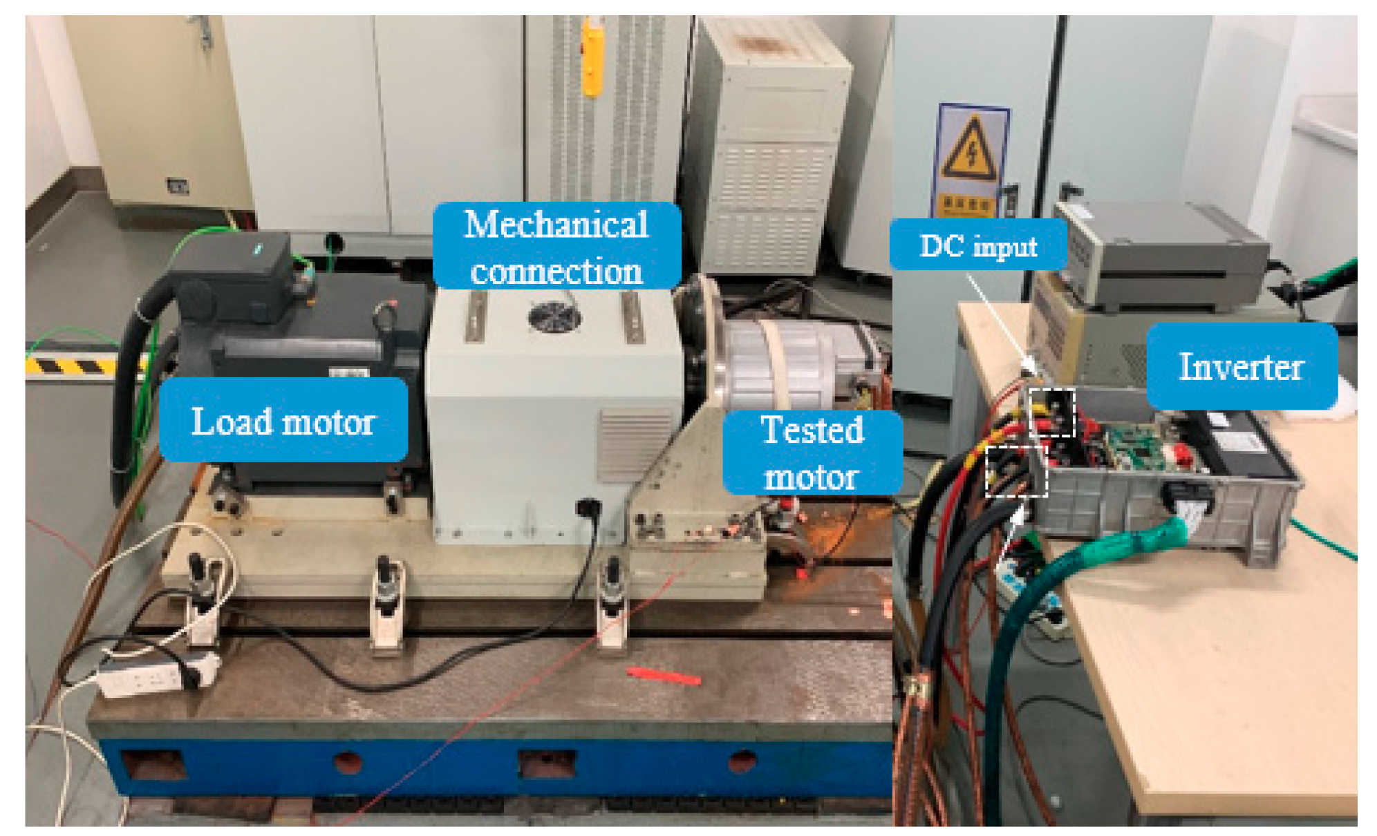
4. Experimental Results

The experimental drive setup consists of a 0.4 kW PMSM connected to a dynamometer machine and a load motor used for loading. The PMSM has a rotor with surface-mounted magnets, the parameters of PMSM are shown in

Table 1. Parameters of tested permanent magnet synchronous motor (PMSM).

Parameter Name	Value
$L_d$	0.322 mH
$L_q$	0.322 mH
${\lambda }_f$	0.011 Wb
$R_s$	0.0113 Ω
$P$	4
$U_N$	36 V
$T_N$	1.27 N·m
$B_f$	0.002 kg·m2

.

Both of load motor and tested motor are supplied by a inverter which is connected with a common DC link and controlled by Infineon TC1782, the sampling-time and PWM frequency is f_s = 10 kHz and the code is written in C Language. Figure 8 shows the photograph of PMSM experimental platform.

This drive uses the proposed current prediction and compensation controllers in a synchronous frame, with constant d-current reference $i_d^{*}=0$.

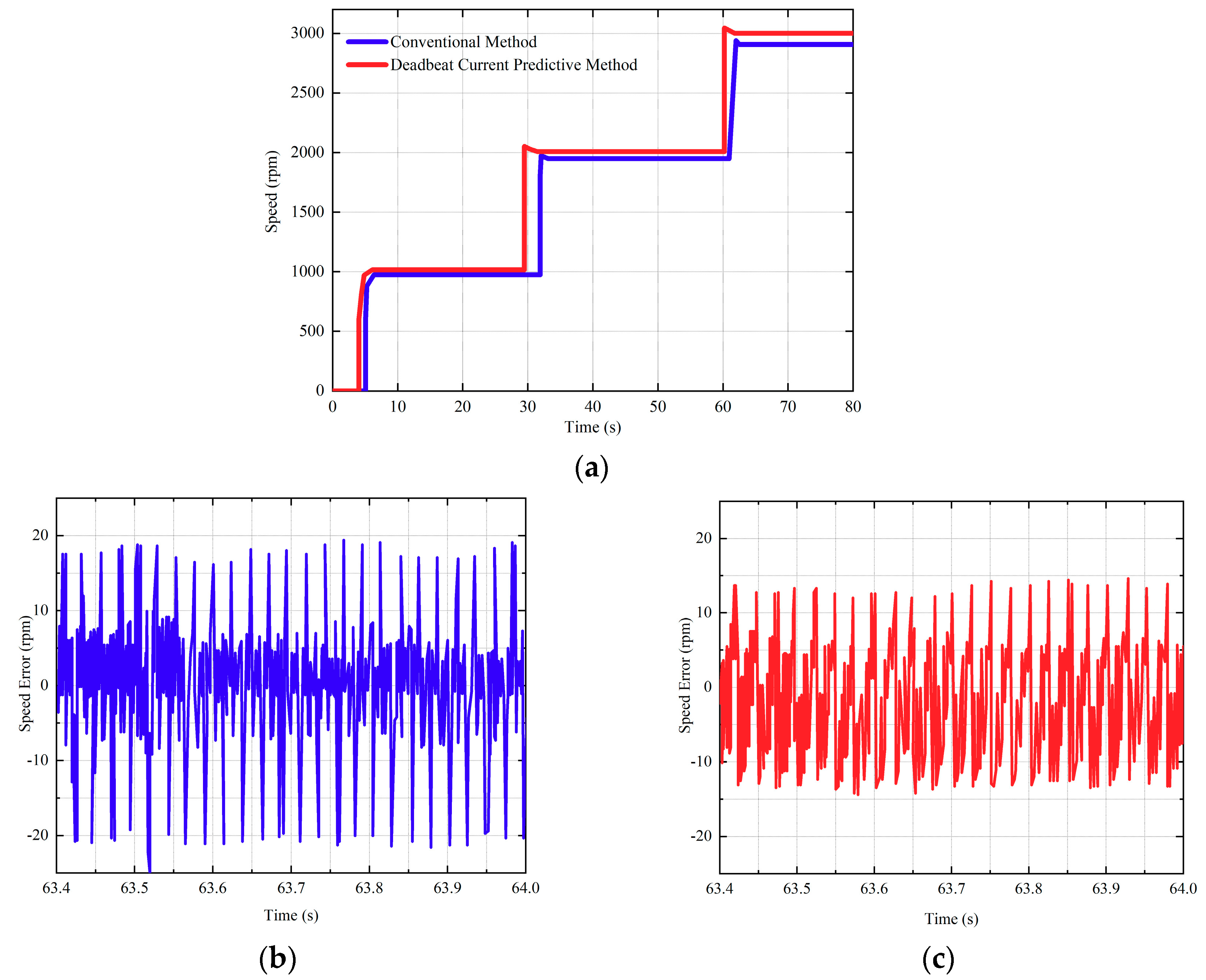
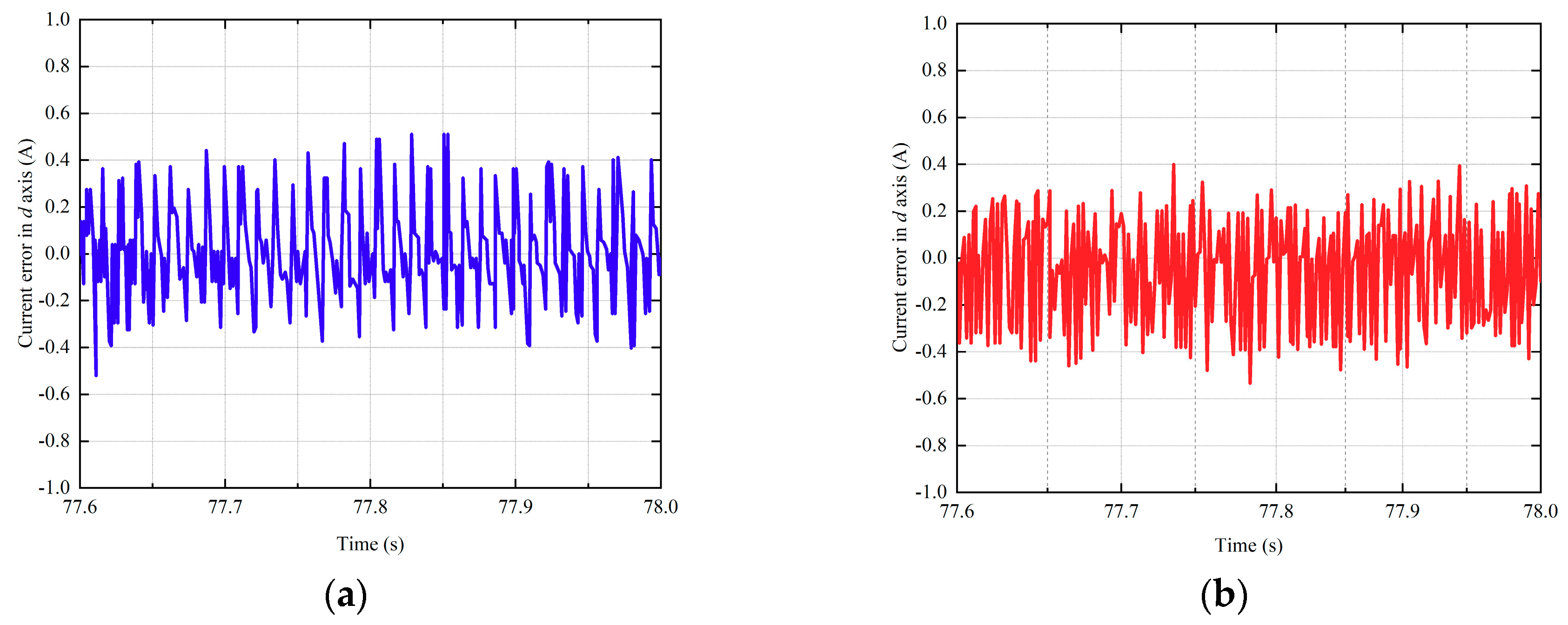
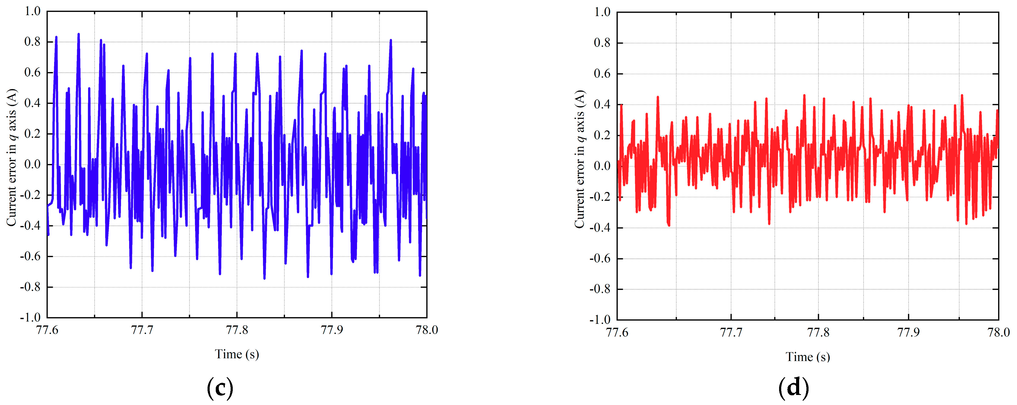
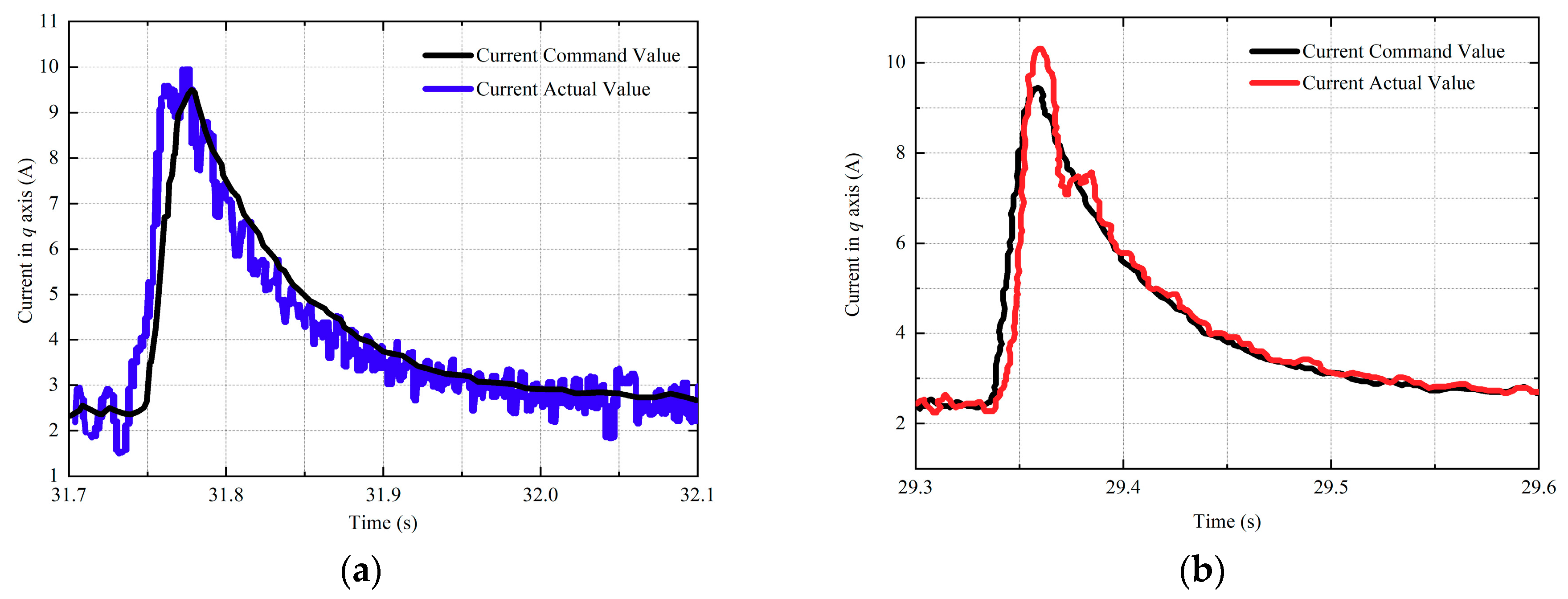
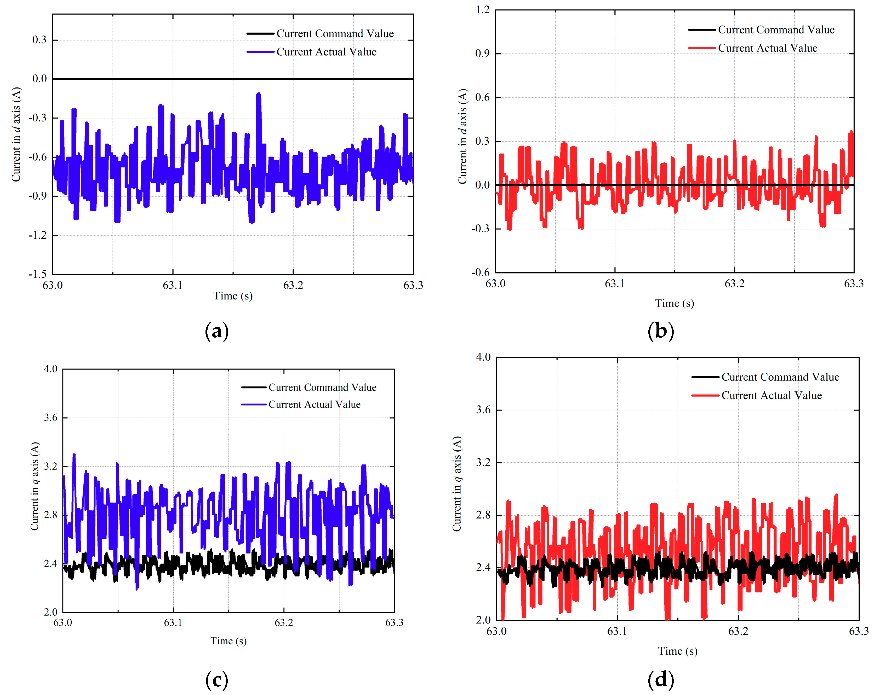
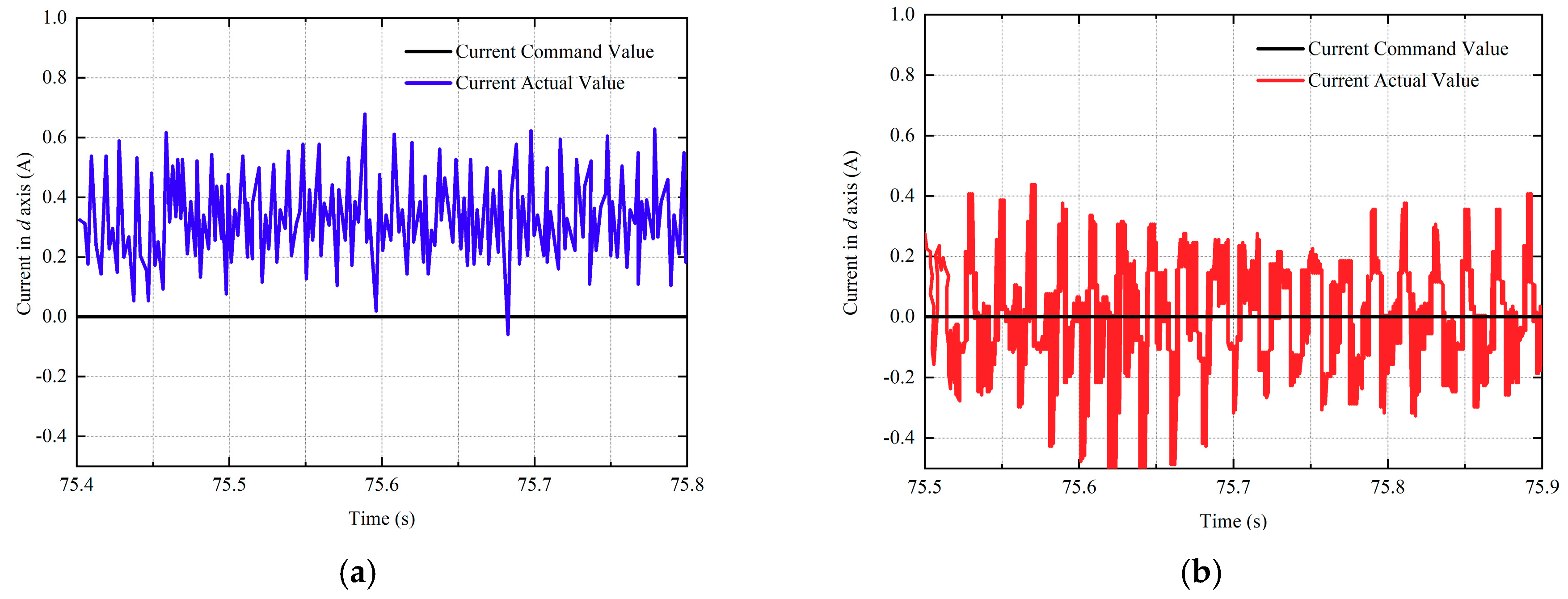
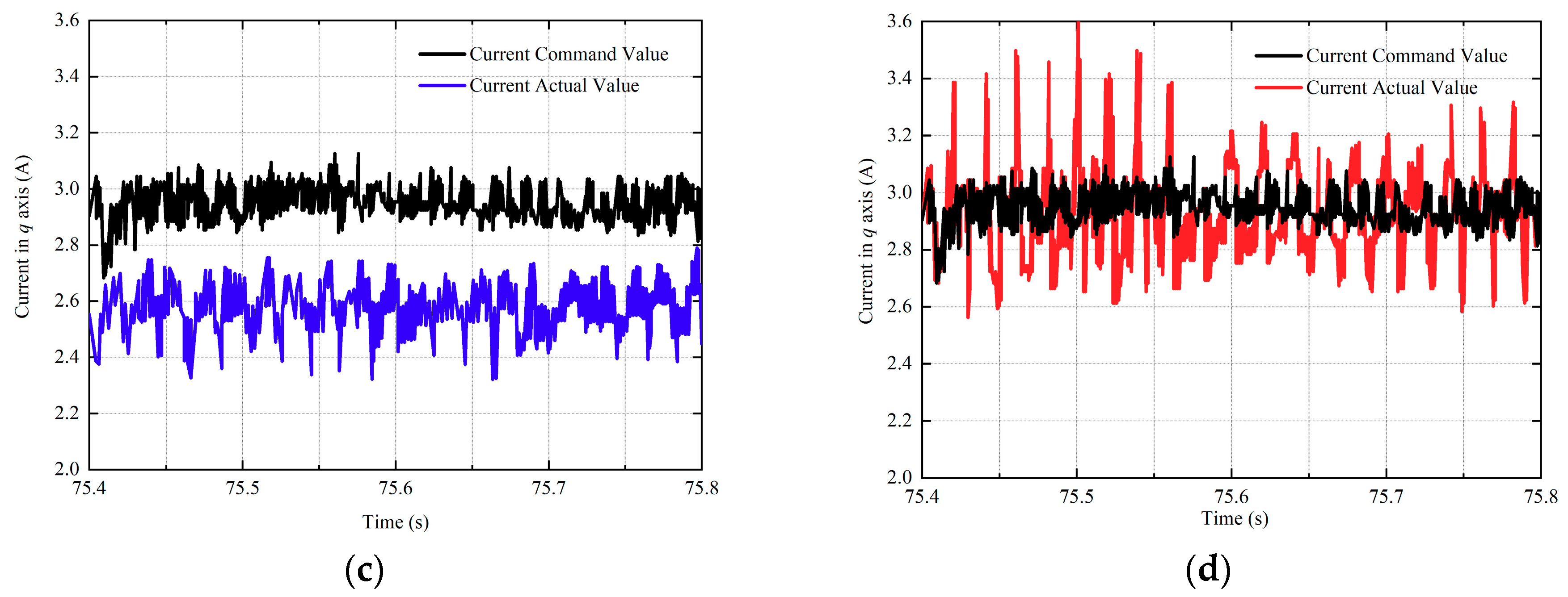
4.1. Experimental Results of Deadbeat-Current Predictive Control Method

In this article, two current predictive control methods are referred, one is conventional predictive method, the other is deadbeat-current predictive method, which is the new method designed in this article. In order to show the advantage of deadbeat control, the experiments based on same operating condition are conducted by 2 different predictive methods.

Figure 9a shows the speed response of 2 current predictive methods in dynamic-state operation at 1000 r/min, 2000 r/min and 3000 r/min with step signal at 5 s, 30 s and 60 s, respectively and a rated load of 0.2 N·m. Figure 9b,c show speed error of 2 current predictive methods in steady-state operation at 3000 r/min with a rated load of 0.2 N$\cdot$m. Although the rotor speed response of PMSM in Figure 9a based on both 2 methods can follow the speed command value, Figure 9b,c show that the speed error by deadbeat predictive control is smaller than conventional methods and can be controlled within 20 rpm and the error fluctuation is also smaller than conventional methods.

As depicted in Figure 9, the fluctuation of current error based on deadbeat-current predictive method is smaller, especially in q-axis and the current error based on new control strategy is within 0.4 A, which can reduce motor system vibration effectively.

Figure 10 shows the current error based on two different current predictive control methods with 0.2 N·m load in 3000 rpm steady-state. Figure 10a,b show the current error in d-axis based on two different current predictive control methods and Figure 10c,d show the current error in q-axis based on two different current predictive control methods.

Figure 11 shows the current response in q-axis based on 2 different methods when the speed command value is changed from 2000 rpm to 3000 rpm suddenly. Obviously, the current response based on new methods shows better performance for its smaller fluctuation.

4.2. Experimental Results of the Proposed Current Compensation with the System Parameter Fluctuation

In order to prove the current compensation effect to reduce the current error caused by parameter fluctuation, the experiment in this part is conducted by setting the motor parameter in controller as 1.5 times higher than actual PMSM: ${\lambda }_f^{\prime }=1.5{\lambda }_f$, $L_d^{\prime }=1.5L_d$, $L_q^{\prime }=1.5L_q$.

Figure 12a,c show experimental current before adding the compensation value, Figure 12b,d show compensated current. All of these experiments are based on inductance change in controller. Apparently, compared with no compensated current, compensated current is closer to current command value and the steady current error is smaller than no compensated value. Hence, the compensation algorithm proposed in this article shows satisfied performance on suppression of inductances fluctuation.

The experiment for PM flux change of PMSM is also conducted by changing the motor PM flux value in controller as ${\lambda }_f^{\prime }=1.5{\lambda }_f$. Figure 13 shows the current response in d- and q-axis, respectively. Apparently, compared with no compensated current, compensated current is closer to current command value, the steady current error is smaller than no compensated value. Hence, the compensation algorithm proposed in this article shows satisfied performance on suppression of PM flux fluctuation.

Noticing that the current response of the deadbeat-current predictive control in all figures shows a quick overshoot, the overshoot can be decreased by choosing appropriate gain in current compensation integrator, but the system settling time will be extended.

Based on all experimental result, the proposed current compensation method in this article indicates the ability to reduce the current error caused by parameter fluctuation.

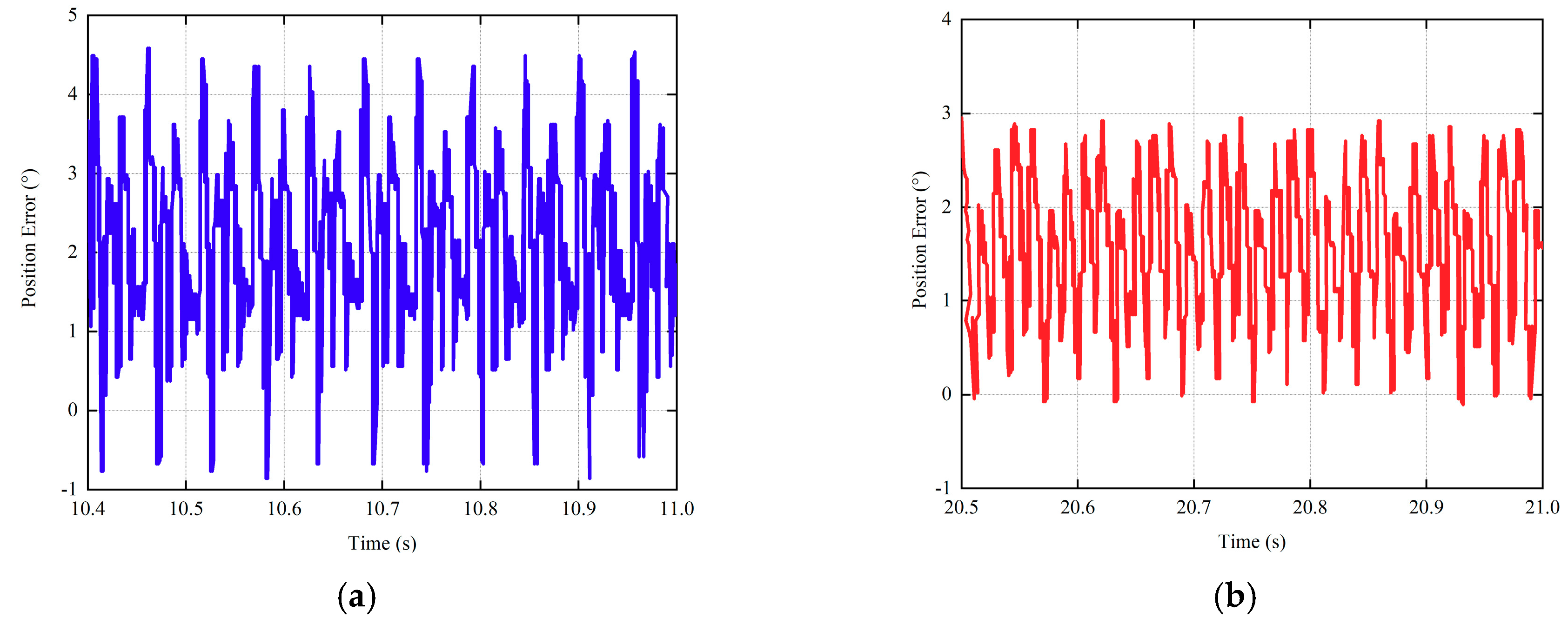
4.3. Experimental Results of Rotor Position and Speed Sensorless Observer

In this article, Luenberger observer and PLL position tracker is applied to estimate rotor position. In order to prove the accuracy of estimated position information, the position error is set as an important index to evaluate the accuracy. The experiment is conducted in 3 different steady-state operations with no load and 0.4 N$\cdot$m load, respectively.

Figure 14a,c,e shows the position error in 1000 rpm, 2000 rpm and 3000 rpm without load, respectively, and Figure 14b,d,f shows the position error in 1000 rpm, 2000 rpm and 3000 rpm with 0.4 N·m load, respectively. The result indicates that position error can be controlled within ± 4° in different steady-states, no matter there is load or not.

5. Conclusions

In this article, a Luenberger rotor sensorless observer based on a proposed current control method is built for the wide-speed-range operation. The conclusions of this paper are listed as follows:

• To solve the phase-lag of estimated extended back-EMF, Luenberger observer and second-order PLL position tracker, in rotational frame, are applied to observe the rotor position and speed, because extended back-EMF signal in rotational frame is a DC signal.
• A deadbeat-current predictive method, by predicting current change is linear within one predictive control period, is proposed to obtain real-time voltage command value.
• Due to the unavoidable parameter fluctuation of PMSM during operation, a current compensation method is proposed, which can reduce current error caused by parameter fluctuation. The method of determining the gain in integrator is designed by system stability.
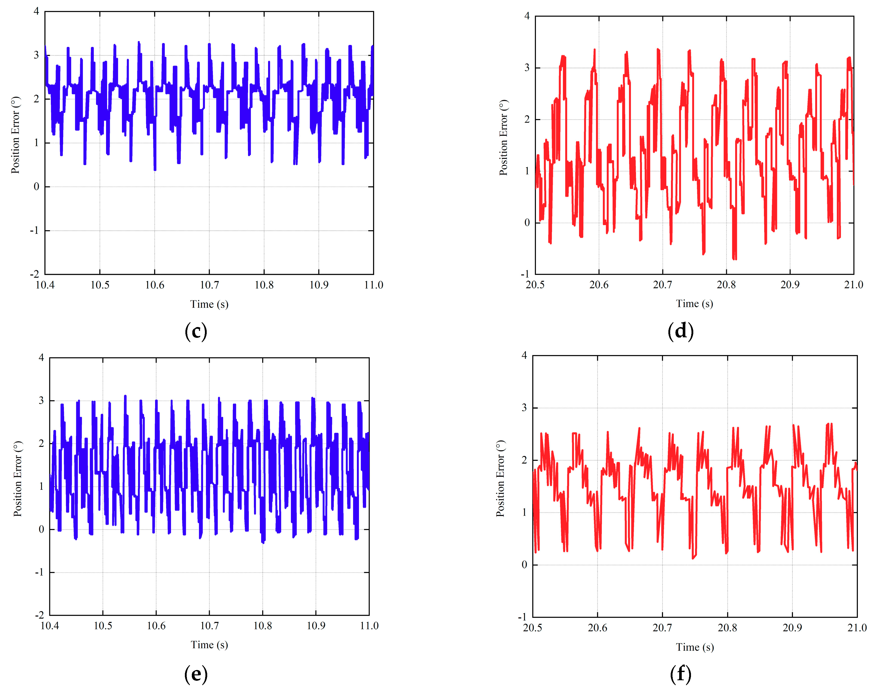
• Finally, the effectiveness and the robustness of the proposed control system are verified. The experimental results show the static and dynamic performance of the new current controller. In the meanwhile, the accuracy of estimated position is proved as well, and the minimum position error can be controlled within ±4° whether the load is given or not.

References

1. Zhu, Y.; Xiao, M.; Su, X.; Lu, K.; Wu, Z.; Yang, G. IGBT Junction Temperature Measurement Under Active-Short-Circuit and Locked-Rotor Modes in New Energy Vehicles. IEEE Access 2020, 8, 114401–114412. [Google Scholar] [CrossRef]
2. Sul, S.K.; Kwon, Y.C.; Lee, Y. Sensorless control of IPMSM for last 10 years and next 5 years. CES Trans. Elect. Mach. 2017, 1, 91–99. [Google Scholar] [CrossRef]
3. Xu, D.; Wang, B.; Zhang, G.; Wang, G.; Yu, Y. A review of sensorless control methods for AC motor drives. CES Trans. Elect. Mach. Syst. 2018, 2, 104–115. [Google Scholar]
4. Yeoh, S.S.; Yang, T.; Tarisciotti, L.; Hill, C.I.; Bozhko, S.; Zancheta, P. Permanent-magnet machine-based starter-generator system with modulated model predictive control. IEEE Trans. Transp. Electrific. 2017, 3, 878–890. [Google Scholar] [CrossRef]
5. Zhu, Y.; Xiao, M.K.; Lu, K.; Wu, Z.H.; Tao, B. A Simplified Thermal Model and Online Temperature Estimation Method of Permanent Magnet Synchronous Motors. Appl. Sci. 2019, 9, 3158. [Google Scholar] [CrossRef] [Green Version]
6. Chen, Z.; Tomita, M.; Doki, S.; Okuma, S. An extended electromotive force model for sensorless control of IPMSM. IEEE Trans. Ind. Electron. 2003, 50, 288–295. [Google Scholar] [CrossRef]
7. Qiao, Z.; Shi, T.; Wang, Y.; Yan, Y.; Xia, C.; He, X. New sliding-observer for position sensorless control of permanent-magnet synchronous motor. IEEE Trans. Ind. Electron. 2013, 60, 710–719. [Google Scholar] [CrossRef]
8. Bierhoff, M. A general PLL-type algorithm for speed sensorless control of electrical drives. IEEE Trans. Ind. Electron. 2017, 64, 9253–9260. [Google Scholar] [CrossRef]
9. Lee, Y.; Sul, S. Model-Based Sensorless Control of IPMSM Enhancing Robustness Based on the Estimation of Speed Error. In Proceedings of the SLED Conference, Nadi, Fiji, 5–6 June 2016. [Google Scholar]
10. Shi, C.; Wang, C. Sensorless vector control of three-phase permanent magnet synchronous motor based on Model-Reference-Adaptive-System. In Proceedings of the 2018 IEEE 4th International Conference on Control Science and Systems Engineering (ICCSSE), Wuhan, China, 21–23 August 2018. [Google Scholar]
11. Zhu, G.; Kaddouri, A.; Dessaint, L.; Akhrif, O. A nonlinear state observer for the sensorless control of a permanent-magnet AC-machine. IEEE Trans. Ind. Electron. 2001, 48, 1098–1108. [Google Scholar]
12. Yao, Y.; Peng, F.; Huang, Y. Position and capacitor voltage sensorless control of high-speed surface-mounted PMSM drive with output filter. In Proceedings of the ECCE Conference, Portland, OR, USA, 23–27 September 2018. [Google Scholar]
13. Li, H.; Wang, Z. Sensorless Control for PMSM Drives Using the Cubature Kalman Filter Based Speed and Flux Observer. In Proceedings of the 2018 IEEE International Conference on Electrical Systems for Aircraft, Railway, Ship Propulsion and Road Vehicles & International Transportation Electrification Conference (ESARS-ITEC), Nottingham, UK, 7–9 November 2018. [Google Scholar]
14. Yang, J.; Mao, Y.; Chen, Y. Sensorless control of permanent magnet synchronous motors with compensation for parameter uncertainty. J. Electr. Eng. Technol. 2017, 12, 1166–1176. [Google Scholar] [CrossRef] [Green Version]
15. Mao, Y.; Yang, J.; Yin, D.; Chen, Y. Sensorless interior permanent magnet synchronous motor control with rotational inertia adjustment. SAGE Adv. Mech. Eng. 2017, 9, 1–9. [Google Scholar] [CrossRef]
16. Solsona, J.; Valla, M.; Muravchik, C. Nonlinear control of a permanent magnet synchronous motor with disturbance torque estimation. IEEE Trans Energy Convers. 2000, 15, 163–168. [Google Scholar] [CrossRef]
17. Yang, S.; Chen, G. High-Speed position-sensorless drive of permanent magnet machine using discrete-time EMF estimation. IEEE Trans. Ind. Electron. 2017, 64, 4444–4453. [Google Scholar] [CrossRef]
18. Liu, J.; Gong, C.; Han, Z.; Yu, H. IPMSM model predictive control in flux weakening operation using an improved algorithm. IEEE Trans. Ind. Electron. 2018, 65, 9378–9387. [Google Scholar] [CrossRef]
19. Zhang, Z.; Fang, H.; Gao, F.; Rodriguez, J.; Kennel, R. Multiple vector model predictive power control for grid-tied wind turbine system with enhanced steady-state control performance. IEEE Trans. Ind. Electron. 2017, 64, 6287–6298. [Google Scholar] [CrossRef]
20. Wang, Y. Deadbeat model-predictive torque control with discrete space-vector modulation for PMSM drives. IEEE Trans. Ind. Electron. 2018, 64, 3537–3547. [Google Scholar] [CrossRef]
21. Suul, J.; LjØkelsØy, K.; Midstund, T.; Undeland, T. Synchronous reference frame hysteresis current control for grid converter applications. IEEE Trans. Ind. Electron. 2011, 47, 2183–2194. [Google Scholar] [CrossRef]
22. Kazmierkowski, M.; Malesani, L. Current control techniques for three-phase voltage-source PWM converters: A survey. IEEE Trans. Ind. Electron. 1998, 45, 691–793. [Google Scholar] [CrossRef]
23. Zhang, Y.; Yang, H. Two-vector-based model predictive torque control without weighting factors for induction motor drives. IEEE Trans. Ind. Electron. 2016, 31, 1381–1390. [Google Scholar] [CrossRef]
24. Zhang, Y.; Yang, H. Generalized two-vector-based Model predictive torque of induction motor drives. IEEE Trans. Power. Electron. 2015, 29, 6593–6630. [Google Scholar] [CrossRef]
25. Zhang, Y.; Yang, H. Model Predictive torque control of induction motor drives with optimal duty cycle control. IEEE Trans. Ind. Electron. 2014, 31, 1381–1390. [Google Scholar] [CrossRef]
26. Liu, H.; Li, S. Speed control for PMSM servo system using predictive functional control and extended state observer. IEEE Trans. Ind. Electron. 2012, 59, 1171–1183. [Google Scholar] [CrossRef]
27. Guzinski, J.; Aburub, H. Speed seneorless induction motor drive with predictive current controller. IEEE Trans. Ind. Electron. 2013, 60, 699–799. [Google Scholar] [CrossRef]
28. Niu, L.; Yang, M.; Xu, D. An adaptive robust model predictive current control for PMSM with online inductance identification. Int. Rev. Elect. Eng. 2012, 7, 3845–3856. [Google Scholar]
29. Chen, W.; Ballance, D.; Gawthrop, P.J.; Gribble, J.J.; O’Reilly, J. Design of a prediction-accuracy-enhanced continuous-time MPC for disturbed system via a disturbance observer. IEEE Trans. Ind. Electron. 2015, 62, 5807–5816. [Google Scholar]
30. Wipasuramonton, P.; Zhu, Z.; Howe, D. Predictive current control with current-error correction for PM brushless AC drives. IEEE Trans. Ind. Appl. 2006, 42, 1071–1079. [Google Scholar] [CrossRef]
31. Lehuy, H.; Slimani, K.; Viarouge, P. Analysis and implementation of a real-time predictive current controller for permanent-magnet synchronous servo drives. IEEE Trans. Ind. Electron. 1994, 41, 110–117. [Google Scholar]
32. Tong, L. An SRF-PLL-based sensorless vector control using the predictive deadbeat algorithm for the direct-driven permanent magnet synchronous generator. IEEE Trans. Power. Electron. 2014, 29, 2837–2849. [Google Scholar] [CrossRef]
Figure 1. Real static coordinate ( α β ) real rotational coordinate (d-q) and estimated rotational coordinate ( γ δ ) for permanent magnet synchronous motor (PMSM).
Electronics 09 01325 g001
Figure 2. The structure of extended back electromotive force (back-EMF) Luenberger observer.
Electronics 09 01325 g002
Figure 3. Structure of phased-locked loop for position tracker based on the estimated extended back-EMF.
Electronics 09 01325 g003
Figure 4. Equivalent structure of phased-locked loop for position tracker.
Electronics 09 01325 g004
Figure 5. Current predictive period analysis based on PWM time-sequence.
Electronics 09 01325 g005
Figure 6. Current compensation within one control period based on closed-loop control of PMSM.
Electronics 09 01325 g006
Figure 7. The whole proposed PMSM control method.
Electronics 09 01325 g007
Figure 8. Photograph of the testing platform.
Electronics 09 01325 g008
Figure 9. Speed response and speed error based on 2 different predictive control at 0.2 N m load. (a) Speed response in dynamic state operation; (b) speed error at 3000 rpm based on conventional method; (c) speed error at 3000 rpm based on deadbeat current predictive method.
Electronics 09 01325 g009
Figure 10. Current error based on 2 different predictive control at 0.2 N m load. (a) Current error in d axis based on conventional method; (b) current error in d axis based on deadbeat current predictive method; (c) current error in q axis based on conventional method; (d) current error in q axis based on deadbeat current predictive method.
Electronics 09 01325 g010aElectronics 09 01325 g010b
Figure 11. Current response in q axis when speed command suddenly changed from 2000 rpm to 3000 rpm. (a) Current response based on conventional method; (b) Current response based on deadbeat current predictive method.
Electronics 09 01325 g011
Figure 12. Current response comparison based on inductances change in controller L d = 1.5 L d L q = 1.5 L q . (a) Current response in d axis before compensation; (b) current response in d axis after compensation; (c) Current response in q axis before compensation; (d) current response in q axis after compensation.
Electronics 09 01325 g012
Figure 13. Current response comparison based on flux linkage changed in controller λ f = 1.5 λ f . (a) Current response in d axis before compensation; (b) Current response in d axis after compensation; (c) Current response in q axis before compensation; (d) Current response in q axis after compensation.
Electronics 09 01325 g013aElectronics 09 01325 g013b
Figure 14. Rotor position error. (a) Rotor position error based on 1000 rpm and no load operation; (b) rotor position error based on 1000 rpm and 0.4 N m load operation; (c) rotor position error based on 2000 rpm and no load operation; (d) rotor position error based on 2000 rpm and 0.4 N m load operation; (e) rotor position error based on 3000 rpm and 0.4 N m load operation; (f) rotor position error based on 3000 rpm and 0.4 N m load operation.
Electronics 09 01325 g014aElectronics 09 01325 g014b