A Novel Data-Driven Specific Emitter Identification Feature Based on Machine Cognition


Abstract
:1. Introduction
2. 2D Transform Domain Feature
2.1. Primitive Transform Domain Feature
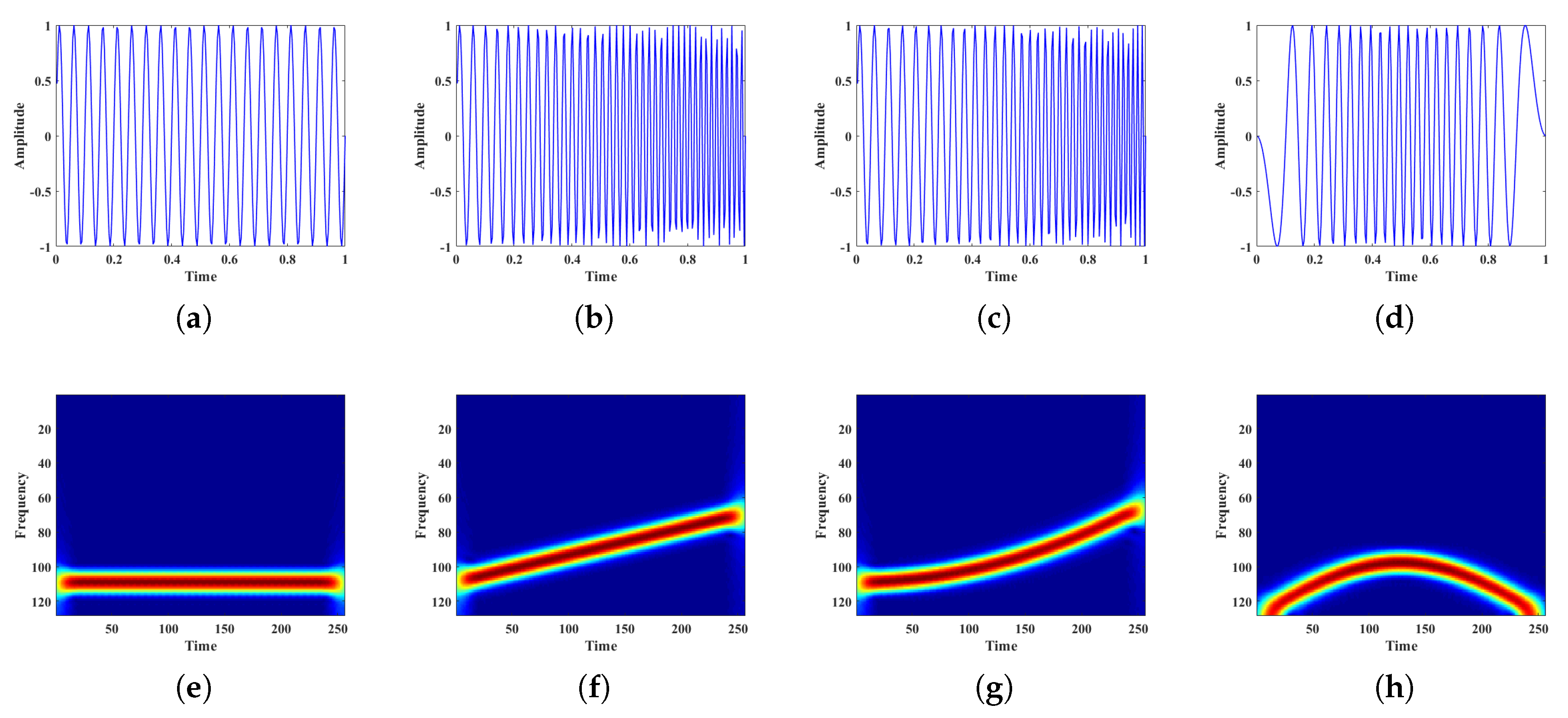
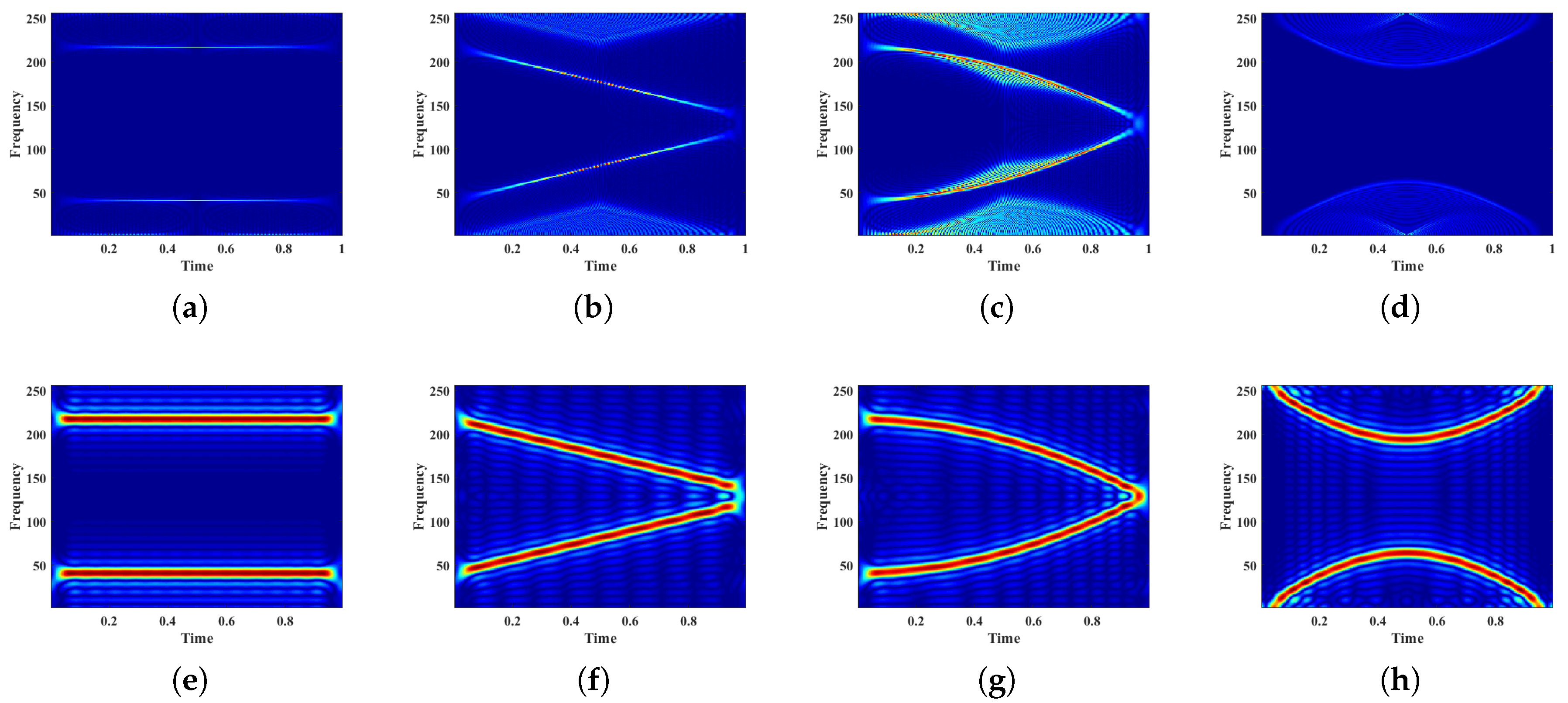
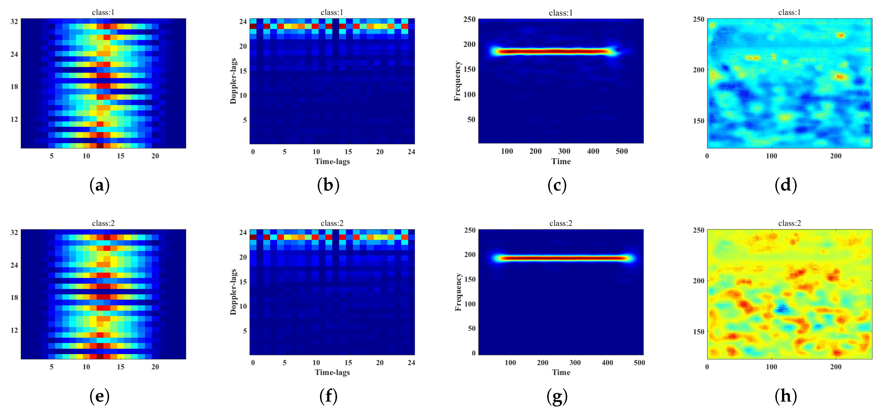
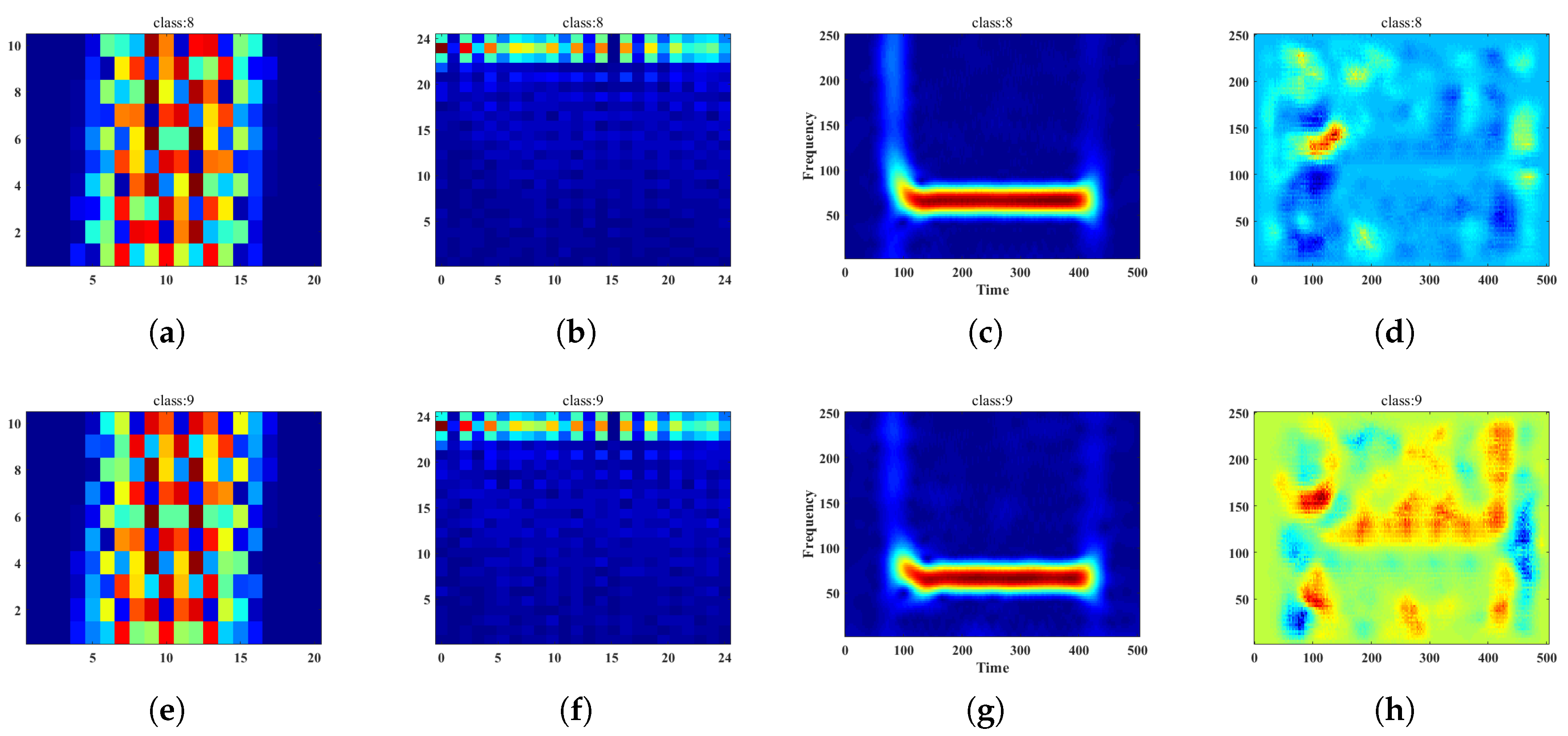
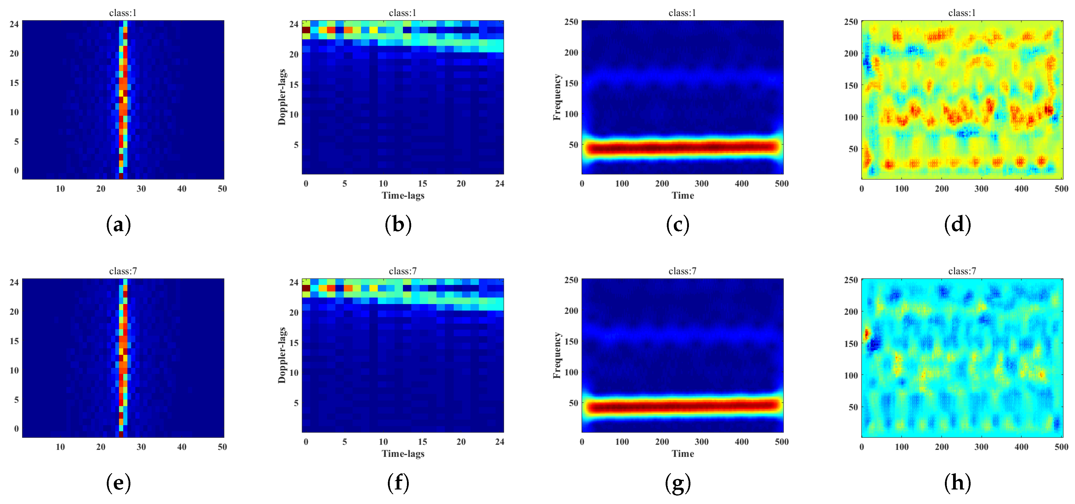
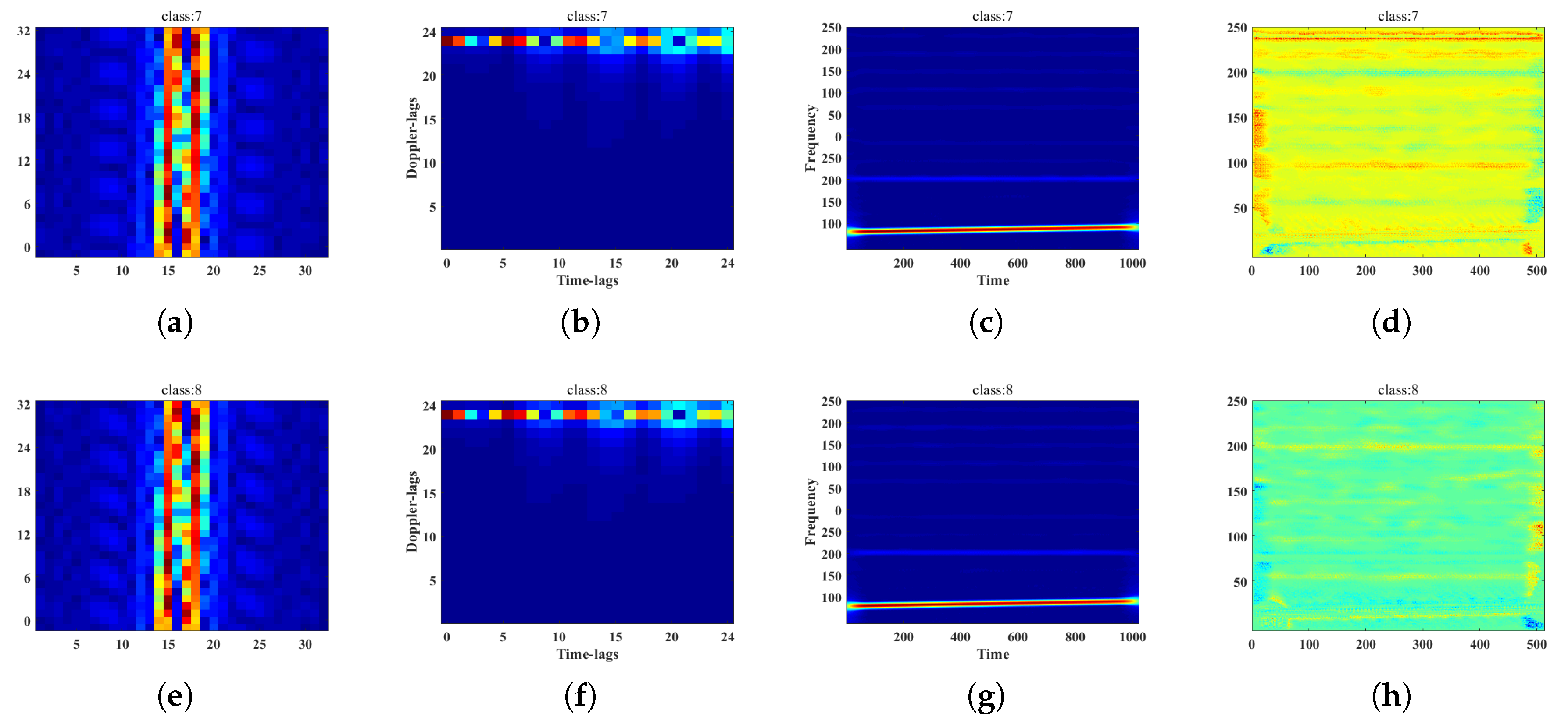
2.1.1. Short Time Fourier Transform
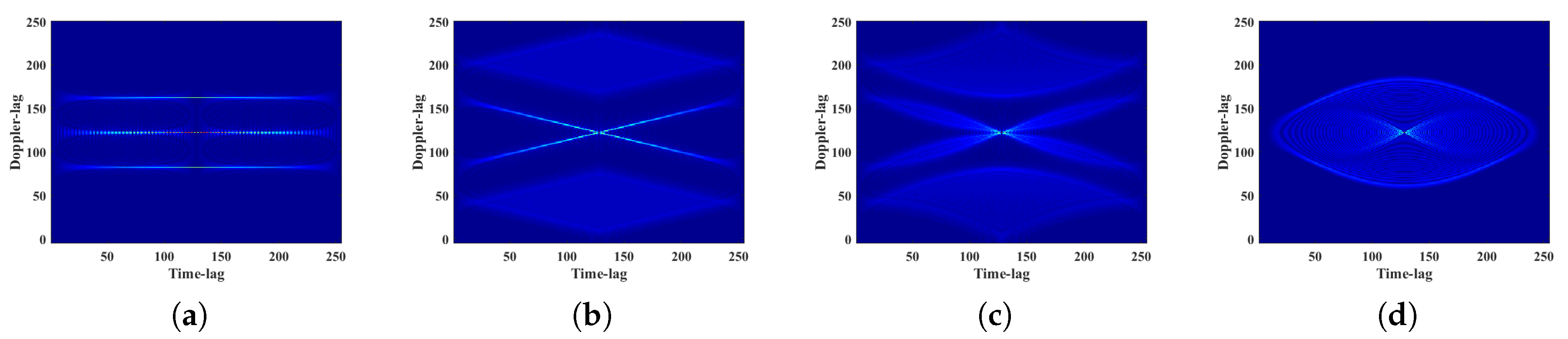
2.1.2. Ambiguity Function
2.2. Handcrafted Transform Domain Feature
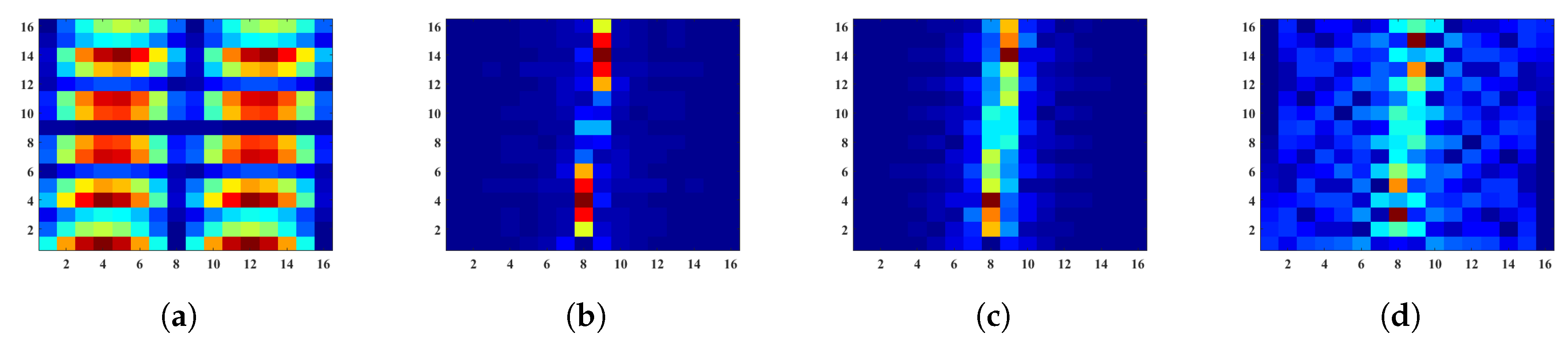
2.2.1. Representative Slice of Ambiguity Function
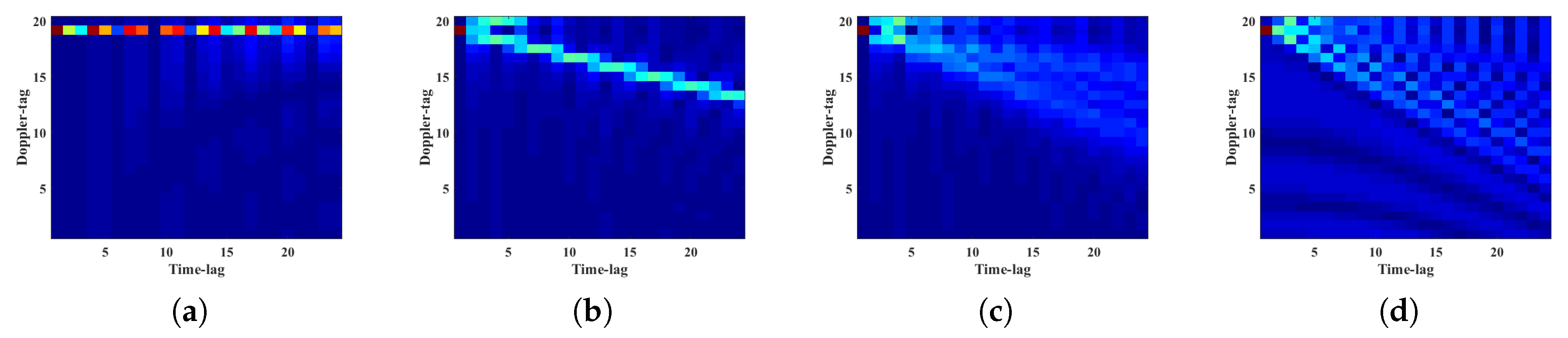
2.2.2. Compressed Sensing Mask
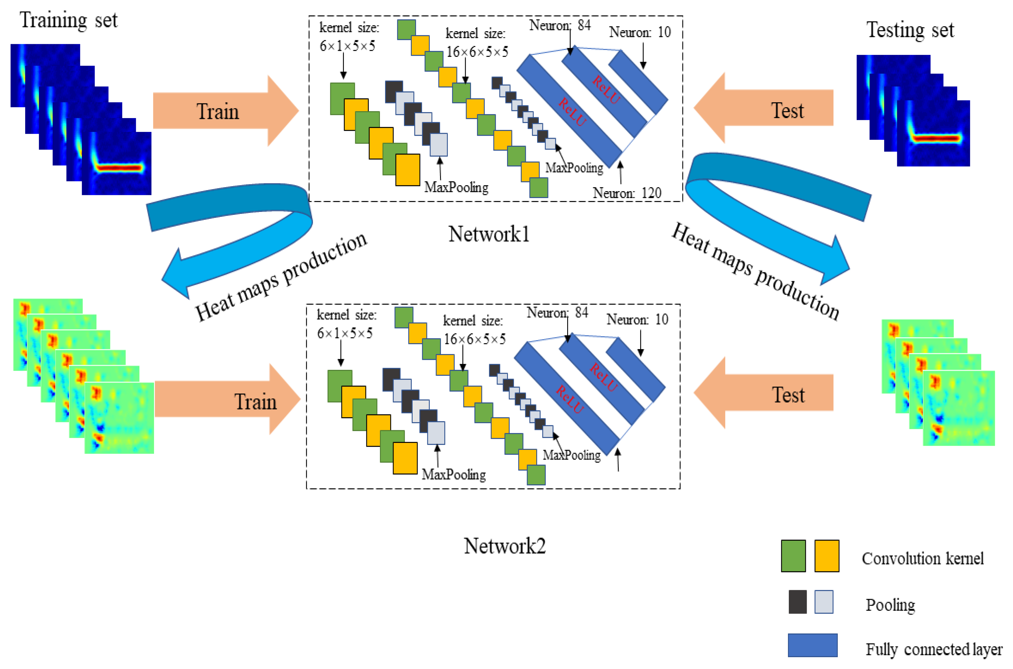
3. MC-Feature
3.1. Image-Specific Class Saliency Visualisation
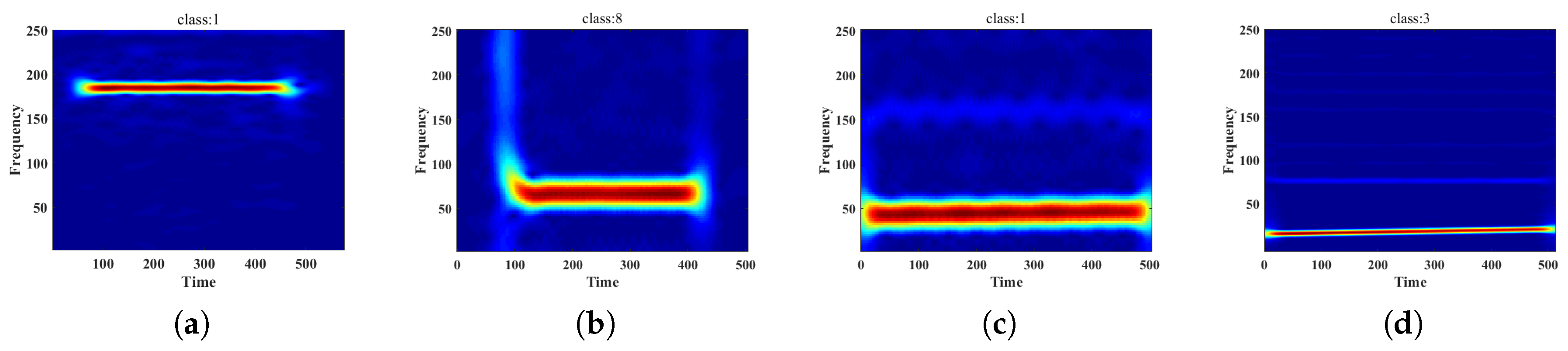
3.2. Saliency Map
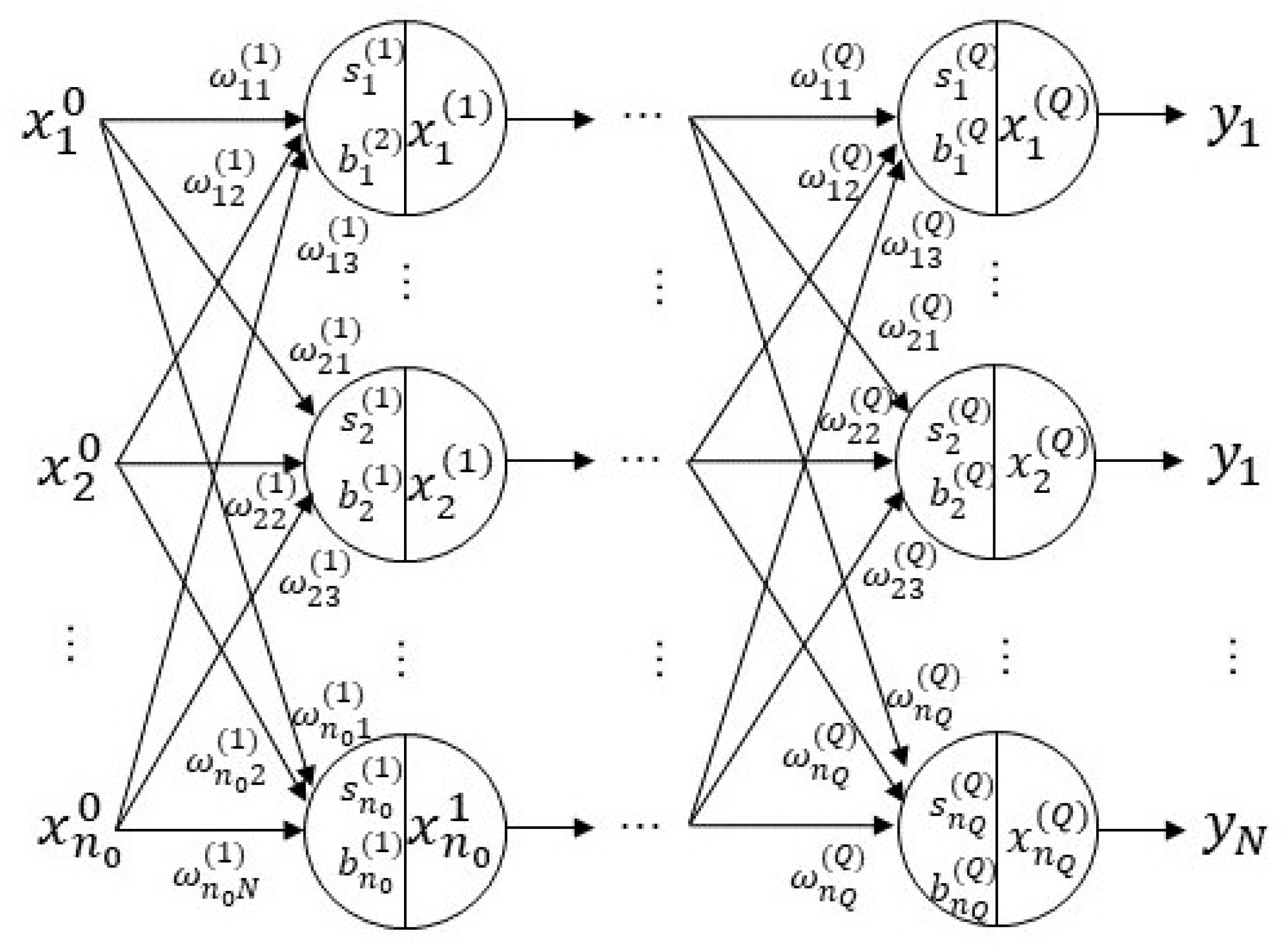
3.3. MC-Feature
| Algorithm 1: Machine Cognition Based Feature Extraction |
| Input: V the transform feature of radar signals in size of (N,C,W,H) as well as corresponding labels L in size of (N,l), N, C, W, H denote the number, channel, width, and height of the , training rate represents a ratio of the number of training set to testing set |
| Step1: Data Partition: Training set: |
| = (1:),= (1:); Testing set: = (+1:N), = (+1:N) |
| Step2: Feed the network1 with and : |
| do: |
| = network1.model() ⊳ train the network with both forward and back propagation |
| = J(, ) ⊳ loss function |
| .backward() |
| while loss > || epoch< K ⊳ is the lowest acceptable loss, and K is the maximum of epochs |
| Obtain a well trained network1 |
| Step3: Saliency maps production: |
| = network1.forward() ⊳ the classification result of network1 |
| .backward() |
| .grad.data |
| Step4: Retrain a new network2 whose structure is identical with network1 |
| Feed the network2 with and |
| Repeat Step2 |
| Obtain a well trained network |
| Step5: Test the network with and |
| Output: network and |
4. Experimental Results
4.1. Data Information
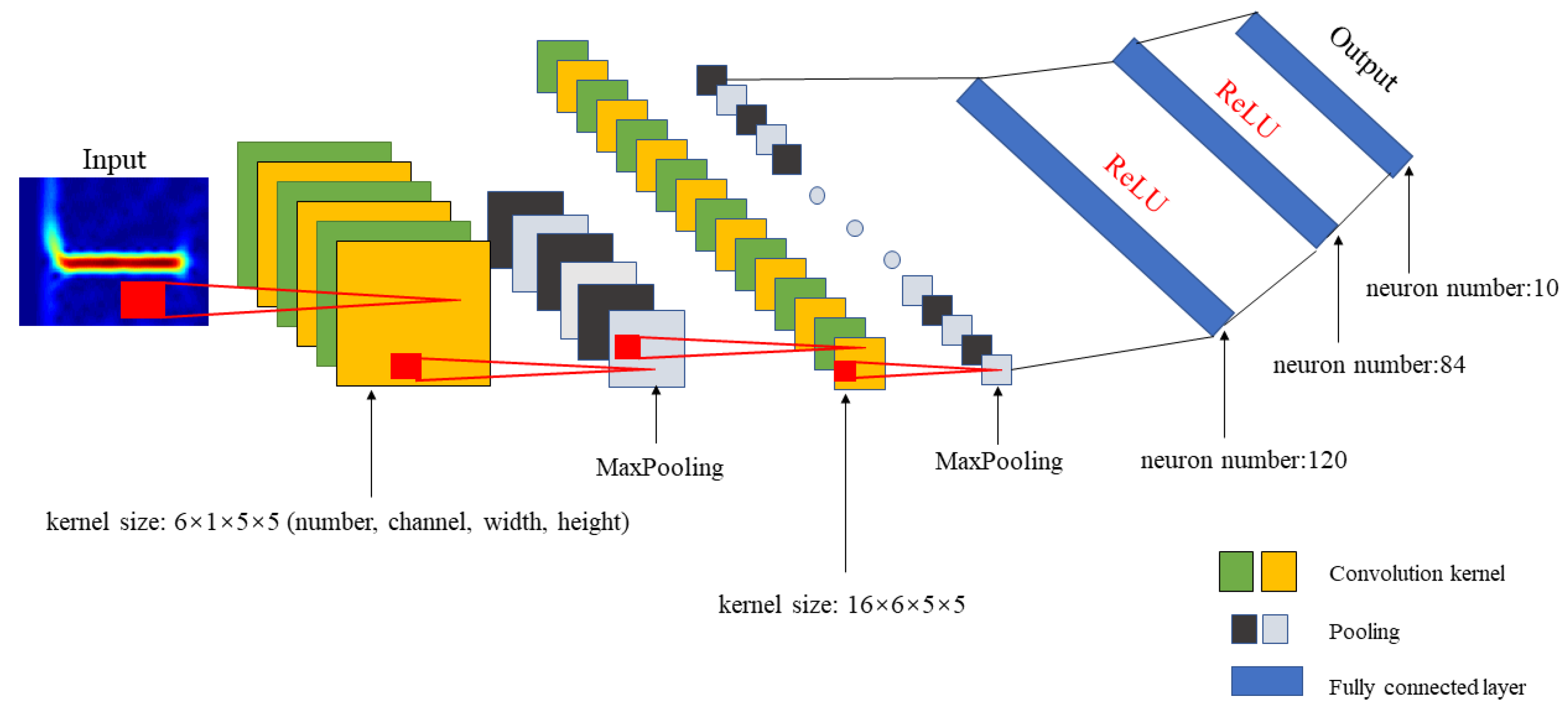
4.2. Recognition CNN Structure
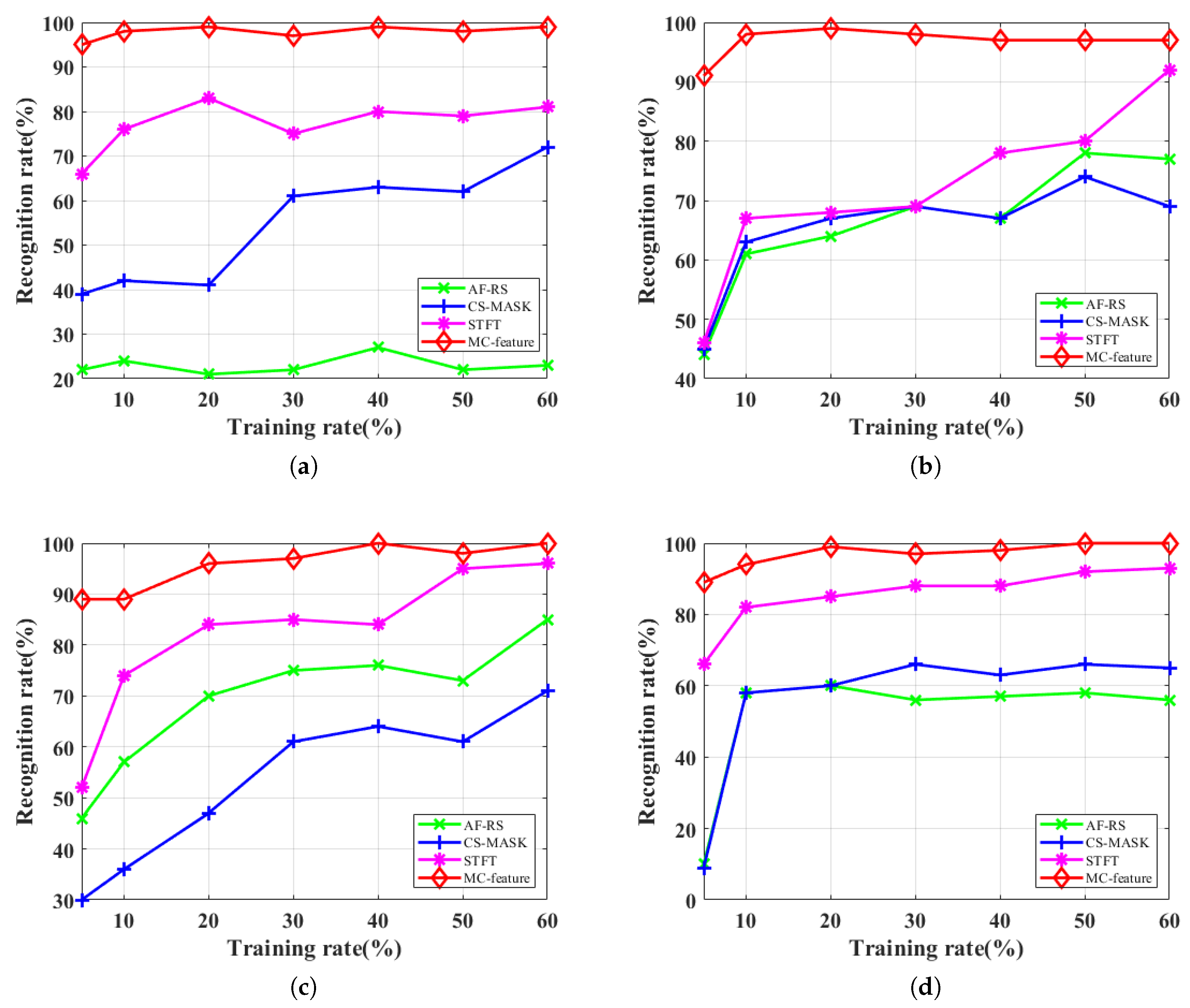
4.3. Results Analysis
5. Conclusions
Author Contributions
Funding
Conflicts of Interest
References
- Yang, L.B.; Zhang, S.S.; Xiao, B. Radar Emitter Signal Recognition Based on Time-frequency Analysis. In Proceedings of the IET International Radar Conference 2013, Xi’an, China, 14–16 April 2013; pp. 1–4. [Google Scholar]
- Lu, J.; Xu, X. Multiple-Antenna Emitters Identification Based on a Memoryless Power Amplifier Model. Sensors 2019, 19, 5233. [Google Scholar] [CrossRef] [PubMed] [Green Version]
- Zhu, M.; Zhou, X.; Zang, B.; Yang, B.; Xing, M. Micro-Doppler Feature Extraction of Inverse Synthetic Aperture Imaging Laser Radar Using Singular-Spectrum Analysis. Sensors 2018, 18, 3303. [Google Scholar] [CrossRef] [PubMed] [Green Version]
- Wang, X.; Huang, G.; Zhou, Z.; Tian, W.; Yao, J.; Gao, J. Radar Emitter Recognition Based on the Energy Cumulant of Short Time Fourier Transform and Reinforced Deep Belief Network. Sensors 2018, 18, 3103. [Google Scholar] [CrossRef] [PubMed] [Green Version]
- Wang, L.; Ji, H.; Shi, Y. Feature Extraction and Optimization of Representative-slice in Ambiguity Function for Moving Radar Emitter Recognition. In Proceedings of the 2010 IEEE International Conference on Acoustics, Speech and Signal Processing (ICASSP), Dallas, TX, USA, 14–19 March 2010; pp. 2246–2249. [Google Scholar]
- Zhu, M.; Zhang, X.; Qi, Y.; Ji, H. Compressed Sensing Mask Feature in Time-Frequency Domain for Civil Flight Radar Emitter Recognition. In Proceedings of the 2018 IEEE International Conference on Acoustics, Speech and Signal Processing (ICASSP), Calgary, AB, Canada, 15–20 April 2018; pp. 2146–2150. [Google Scholar]
- Zhu, M.; Feng, Z.; Zhou, X. Specific Emitter Identification Based on Synchrosqueezing Transform for Civil Radar. Electronics 2020, 9, 658. [Google Scholar] [CrossRef]
- Ayhan, B.; Kwan, C. Robust Speaker Identification Algorithms and Results in Noisy Environments. In Proceedings of the International Symposium on Neural Networks, Minsk, Belarus, 25–28 June 2018. [Google Scholar]
- Wang, D.; Brown, G.J. Computational Auditory Scene Analysis: Principles, Algorithms and Applications. J. Acoust. Soc. Am. 2008, 124, 13. [Google Scholar]
- Misaghi, H.; Moghadam, R.A.; Mahmoudi, A.; Salemi, A. Image Saliency Detection By Residual and Inception-like CNNs. In Proceedings of the 2018 6th RSI International Conference on Robotics and Mechatronics (IcRoM), Tehran, Iran, 23–25 October 2018; pp. 94–99. [Google Scholar]
- Ramik, D.M.; Sabourin, C.; Moreno, R.; Madani, K. A Machine Learning Based Intelligent Vision System for Autonomous Object Detection and Recognition. Appl. Intell. 2014, 40, 94–99. [Google Scholar] [CrossRef]
- Simonyan, K.; Vedaldi, A.; Zisserman, A. Deep Inside Convolutional Networks: Visualising Image Classification Models and Saliency Maps. arXiv 2013, arXiv:1312.6034. [Google Scholar]
- Auger, F.; Flandrin, P.; Lin, Y. Time-Frequency Reassignment and Synchrosqueezing: An Overview. IEEE Signal Process. Mag. 2013, 30, 32–41. [Google Scholar] [CrossRef] [Green Version]
- Gillespie, B.W.; Atlas, L.E. Optimizing Time-Frequency Kernels for Classification. IEEE Trans. Signal Process. 2001, 49, 485–496. [Google Scholar] [CrossRef]
- Gillespie, B.W.; Atlas, L.E. Optimization of Time and Frequency Resolution for Radar Transmitter Identification. In Proceedings of the 1999 IEEE International Conference on Acoustics, Speech, and Signal Processing (ICASSP), Phoenix, AZ, USA, 15–19 March 1999; pp. 1341–1344. [Google Scholar]
- Islam, N.U.; Lee, S. Interpretation of Deep CNN Based on Learning Feature Reconstruction With Feedback Weights. IEEE Access 2019, 7, 25195–25208. [Google Scholar] [CrossRef]
- Kim, J.; Kim, J.; Kim, H.; Shim, M.; Choi, E. CNN-Based Network Intrusion Detection Against Denial-of-Service Attacks. Electronics 2020, 9, 916. [Google Scholar] [CrossRef]
- Lecun, Y.; Bottou, L.; Bengio, Y.; Haffner, P. Gradient-based Learning Applied to Document Recognition. Proc. IEEE 1998, 86, 2278–2324. [Google Scholar] [CrossRef] [Green Version]
- Krizhevsky, A.; Sutskever, I.; Hinton, G. ImageNet Classification with Deep Convolutional Neural Networks. Commun. ACM 2017, 60, 84–90. [Google Scholar] [CrossRef]
- Ciregan, D.; Meier, U.; Schmidhuber, J. Multi-column Deep Neural Networks for Image Classification. In Proceedings of the 2012 IEEE Conference on Computer Vision and Pattern Recognition, Providence, RI, USA, 16–21 June 2012; pp. 3642–3649. [Google Scholar]
- Erhan, D.; Bengio, Y.; Courville, A.; Vincent, P. Visualizing Higher-Layer Features of a Deep Network; Technical Report 1341; University of Montreal: Montreal, QC, Canada, 2009. [Google Scholar]
- Zeiler, M.D.; Fergus, R. Visualizing and Understanding Convolutional Networks. arXiv 2013, arXiv:1311.2901. [Google Scholar]
- Rumelhart, D.E.; Hinton, G.E.; Williams, R.J. Learning Representations By Back-Propagating Errors. Nature 1986, 323, 533–536. [Google Scholar] [CrossRef]
- Wanga, X.; Li, J.; Yang, Y. Comparison of Three Radar Systems for Through-the-Wall Sensing. In Radar Sensor Technology XV; Spie-the International Society for Optical Engineering: Bellingham, WA, USA, 2011. [Google Scholar]
- Yao, Y.; Li, X.; Wu, L. Cognitive Frequency-Hopping Waveform Design for Dual-Function MIMO Radar-Communications System. Sensors 2020, 20, 415. [Google Scholar] [CrossRef] [Green Version]
- Hamran, S.E. Radar Performance of Ultra Wideband Waveforms. In Radar Technology; InTech: Rijeka, Croatia, 2009. [Google Scholar]
- LeCun, Y.; Bengio, Y. Convolutional Networks for Images, Speech, and Time-Series. In The Handbook of Brain Theory and Neural Networks; MIT Press: Cambridge, MA, USA, 1998. [Google Scholar]
- Krizhevsky, A.; Sutskever, I.; Hinton, G. ImageNet Classification with Deep Convolutional Neural Networks. In Advances in Neural Information Processing Systems; MIT Press: Cambridge, MA, USA, 2012. [Google Scholar]
- Simonyan, K.; Zisserman, A. Very Deep Convolutional Networks for Large-Scale Image Recognition. In Proceedings of the International Conference on Learning Representations, San Diego, CA, USA, 7–9 May 2015; pp. 1–14. [Google Scholar]
- Szegedy, C.; Liu, W.; Jia, Y.; Sermanet, P.; Reed, S.; Anguelov, D.; Erhan, D.; Vanhoucke, V.; Rabinovich, A. Going Deeper with Convolutions. In Proceedings of the 2015 IEEE Conference on Computer Vision and Pattern Recognition (CVPR), Boston, MA, USA, 7–12 June 2015; pp. 1–9. [Google Scholar]


| Feature | AF-RS | CS-MASK | STFT | MC-Feature | |
|---|---|---|---|---|---|
|
Training Rate(%) | |||||
| 5 | 22% | 39% | 66% | ||
| 10 | 24% | 42% | 76% | ||
| 20 | 21% | 41% | 83% | ||
| 30 | 22% | 61% | 75% | ||
| 40 | 27% | 63% | 80% | ||
| 50 | 22% | 62% | 79% | ||
| 60 | 23% | 72% | 81% | ||
| Feature | AF-RS | CS-MASK | STFT | MC-Feature | |
|---|---|---|---|---|---|
|
Training Rate(%) | |||||
| 5 | 44% | 45% | 46% | ||
| 10 | 61% | 63% | 67% | ||
| 20 | 64% | 67% | 68% | ||
| 30 | 69% | 69% | 69% | ||
| 40 | 67% | 67% | 78% | ||
| 50 | 78% | 74% | 80% | ||
| 60 | 77% | 69% | 92% | ||
| Feature | AF-RS | CS-MASK | STFT | MC-Feature | |
|---|---|---|---|---|---|
|
Training Rate(%) | |||||
| 5 | 46% | 30% | 52% | ||
| 10 | 57% | 36% | 74% | ||
| 20 | 70% | 47% | 84% | ||
| 30 | 75% | 61% | 85% | ||
| 40 | 76% | 64% | 84% | ||
| 50 | 73% | 61% | 95% | ||
| 60 | 85% | 71% | 96% | ||
| Feature | AF-RS | CS-MASK | STFT | MC-Feature | |
|---|---|---|---|---|---|
|
Training Rate(%) | |||||
| 5 | 10% | 9% | 66% | ||
| 10 | 58% | 58% | 82% | ||
| 20 | 60% | 60% | 85% | ||
| 30 | 56% | 66% | 88% | ||
| 40 | 57% | 63% | 88% | ||
| 50 | 58% | 66% | 92% | ||
| 60 | 56% | 65% | 93% | ||
© 2020 by the authors. Licensee MDPI, Basel, Switzerland. This article is an open access article distributed under the terms and conditions of the Creative Commons Attribution (CC BY) license (http://creativecommons.org/licenses/by/4.0/).
Share and Cite
Zhu, M.; Feng, Z.; Zhou, X. A Novel Data-Driven Specific Emitter Identification Feature Based on Machine Cognition. Electronics 2020, 9, 1308. https://doi.org/10.3390/electronics9081308
Zhu M, Feng Z, Zhou X. A Novel Data-Driven Specific Emitter Identification Feature Based on Machine Cognition. Electronics. 2020; 9(8):1308. https://doi.org/10.3390/electronics9081308
Chicago/Turabian StyleZhu, Mingzhe, Zhenpeng Feng, and Xianda Zhou. 2020. "A Novel Data-Driven Specific Emitter Identification Feature Based on Machine Cognition" Electronics 9, no. 8: 1308. https://doi.org/10.3390/electronics9081308