Optimal Power Flow Incorporating FACTS Devices and Stochastic Wind Power Generation Using Krill Herd Algorithm

Abstract

This paper deals with investigating the Optimal Power Flow (OPF) solution of power systems considering Flexible AC Transmission Systems (FACTS) devices and wind power generation under uncertainty. The Krill Herd Algorithm (KHA), as a new meta-heuristic approach, is employed to cope with the OPF problem of power systems, incorporating FACTS devices and stochastic wind power generation. The wind power uncertainty is included in the optimization problem using Weibull probability density function modeling to determine the optimal values of decision variables. Various objective functions, including minimization of fuel cost, active power losses across transmission lines, emission, and Combined Economic and Environmental Costs (CEEC), are separately formulated to solve the OPF considering FACTS devices and stochastic wind power generation. The effectiveness of the KHA approach is investigated on modified IEEE-30 bus and IEEE-57 bus test systems and compared with other conventional methods available in the literature.

1. Introduction

Optimal Power Flow (OPF) plays a significant role in power systems operation and control. The OPF mainly aims to optimize a certain objective function, such as minimizing the generation fuel cost and at the same time, satisfying the load balance constraints and bound constraints [1,2]. Under normal conditions, all devices in power systems should operate within their pre-determined range. Such constraints include the maximum and minimum active and reactive power of the generation units, voltage levels, loadability of power transmission lines, and transformers tap settings. Minimizing the operating costs and increasing the reliability of power systems are two main objectives from the power companies and utilities’ point of view. Basically, the power flow problem focuses on the economic aspect of operating the power systems due to the fact that a slight change in power flow may significantly increase the operating costs of power systems. To do so, an objective function is optimized considering various equality and inequality constraints. Solving the OPF problem precisely leads to proper control, planning, and protection of power systems. The OPF problem can be divided into two major problems: (1) the optimal active power flow problem, and (2) the optimal reactive power flow problem. Numerous papers have investigated the OPF problem using conventional optimization methods, such as the Newton Raphson (NR) method, and evolutionary optimization techniques, such as particle swarm optimization (PSO) and artificial bee colony (ABC) optimization algorithms.

Increasing the load demand over the last few decades has created different problems in power systems in terms of power transmission congestion and constraints. Those limitations are mainly due to maintaining the stability and maintaining the voltage range of the power system at its permissible level [3,4]. Distributed Generations (DGs) are one of the best solutions to prevent congestion in the transmission lines [5]. DGs have several advantages, such as reducing energy costs, improving power quality and reliability, and preventing environmental pollutions. Among different DGs, wind power is one of the most popular power generations. However, wind behavior is often unpredictable, as it is a stochastic phenomenon, thereby, needing proper uncertainty modeling. To cope with this challenge, many research studies in the literature have investigated different methods to model the random behavior of the wind power generation, as depicted in

Table 1. Different methods to model the random behavior of wind power generations.

Reference	Uncertainty Model	Solution Method	Objective Functions
[6]	Weibull distribution function	Sequential quadratic programming PSO	Minimizing the total operating costs and minimizing emission
[7]	Incomplete gamma function	Imperialist Competitive Algorithm (ICA)	Minimizing the fuel cost function
[8]	Weibull probability density function	Gbest Guided-ABC	Minimizing the total operating costs
[9]	Weibull probability density function	PSO	Minimizing the total operating and congestion costs

.

Another way to enhance the capacity of the transmission systems is by employing Flexible AC Transmission System (FACTS) devices [10]. FACTS devices play a crucial role in improving the flexibility of power transmission and guaranteeing the stability of power systems. FACTS devices are used for improving power flow regardless of the costs of generating power. Two primary goals of using FACTS devices are (1) increasing capacity of transmission systems by controlling some characteristics, such as series/shunt impedances and phase angle; (2) transmitting power through the desired paths.

Table 2. Different methods to model the random behavior of wind power generations.

Reference	Method	Objective Functions	FACTS Devices
[7]	Micro-genetic algorithm and hybrid method	Minimizing the fuel cost and power losses, Optimal location of FACTS devices	TCSC, TCPAR, UPFC, SVC
[8]	PSAT software analysis	Improving voltage profile, Minimizing power losses	SVC
[9]	Dimensional algorithm using NR load flow	Improving voltage profile, Minimizing power losses and fuel costs	TCSC, TCPR, SVC, STATCOM
[11]	Genetic Algorithm (GA) and Differential Evolution Algorithm (DEA)	Minimizing the fuel cost and power losses, Optimal location of FACTS devices	UPFC, SVC, TCSC
[12]	Dimensional algorithm	Heat control, Minimizing power losses, Improving power systems stability	UPFC
[13]	GA and DEA	Minimizing the fuel cost and power losses	UPFC
[14]	Artificial Immune Systems (AIS)	Minimizing the fuel cost	TCPS, TCSC
[15]	GA	Minimizing the fuel cost and power losses	TCSC, TCPAR, UPFC
[16]	DEA	Maximizing the loadability of transmission lines, Reducing the transmission lines losses	STATCOM
[17]	Combined Tabu Search (TS) and Simulated Annealing (SA) method	Minimizing the total fuel cost	TCSC, TCPS
[18]	GA	Minimizing the total fuel costs under security constraints	UPFC
[19]	PSO	Reducing the FACTS devices installation costs, Reducing overload	TCSC, UPFC, SVC, TCVR

shows a summary of the previous research studies related to the FACTS devices. Therefore, the conventional OPF problem, integrated with FACTS devices can open new opportunities for controlling the active and reactive power flow.

To date, numerous papers on the OPF problem with various optimization techniques have been published. However, previous studies have not dealt with the OPF incorporating FACTS devices and stochastic wind power generation at the same time. In this regard, this paper proposes an OPF solution of power system considering FACTS devices and stochastic wind power generation using the krill herd algorithm (KHA). The wind power uncertainty is modeled in the optimization problem using the Weibull probability density function. Minimization of fuel cost, active power losses across the transmission lines, emission, and combined economic and environmental costs (CEEC) are the objective functions.

To the best of the authors’ knowledge, solving the OPF problem considering the minimization of fuel cost, active power losses across transmission lines, emission, and CEEC, incorporating FACTS devices and dealing with the stochastic behavior of wind power generation has not been investigated before. Compared with the other techniques, the proposed method has better performance and achieves more accurate results.

The followings are the major contributions of this research study:

• Modeling and including the stochastic nature of wind power generation in the problem formulation.
• Unlike the other research studies, in this paper, the OPF problem incorporating FACTS devices and stochastic wind power generation at the same time is solved.
• The KHA is used to minimize the fuel cost, active power losses across the transmission lines, emission, and CEEC, as the objective functions.

This paper is divided into four sections. In Section 2, the problem formulation is given. The results are presented in Section 3. Finally, the conclusions are presented.

2. Problem Formulation

In this part, the OPF problem formulation in the presence of FACTS devices, including thyristor controlled phase shifter (TCPS) as well as thyristor-controlled series compensator (TCSC), and stochastic wind power generation is presented. The frequency distribution is one of the most essential tools for planning and operating in power systems, and its general structure is divided into two parts of the objective function and constraints.

2.1. General Formulation

The general formulation for the constrained optimization problem in this paper is as follows:

$$\min f\left(u,v\right)$$

(1)

subject to:

$$\{\begin{array}{c}g\left(u,v\right)=0\\ h\left(u,v\right)\le 0\end{array}$$

(2)

where $f$ is the objective function that should be minimized, $g\left(u,v\right)$ is the set of equality constraints, and $h\left(u,v\right)$ is the set of inequality constraints. It should be noted that for $N$ number of components in power systems, $u$ is the vector of dependent variables that contains the active power of the slack generator, voltage of the loads $\left(V_{L_1},\dots ,V_{L_{N_{PQ}}}\right)$, reactive power generation by the generation units $\left(Q_{G_1},\dots ,Q_{G_{N_{PV}}}\right)$, and the lines loadability $\left(S_{L_1},\dots ,S_{L_{N_L}}\right)$. Also, $v$ is the vector of independent variables that contains active power generation by the generation unit except for the slack bus $\left(P_{G_1},\dots ,P_{G_{N_{PV}}}\right)$, voltage of the generators $\left(V_{G_1},\dots ,V_{G_{N_{PV}}}\right)$, transformers tap settings $\left(T_1,\dots ,T_{N_T}\right)$, and the injected reactive power by the FACTS devices $\left(Q_{C_1},\dots ,Q_{C_{N_C}}\right)$. It should be noted that $N_{PQ}$, $N_{PV}$, $N_L$, $N_T$, and $N_C$ show the maximum number of generation buses, load buses, transmission lines, transformer tap settings, and FACTS devices, respectively.

The constraints of the OPF problem include active and reactive power of the generation units, transformer tap settings, and the loading of the power transmission lines.

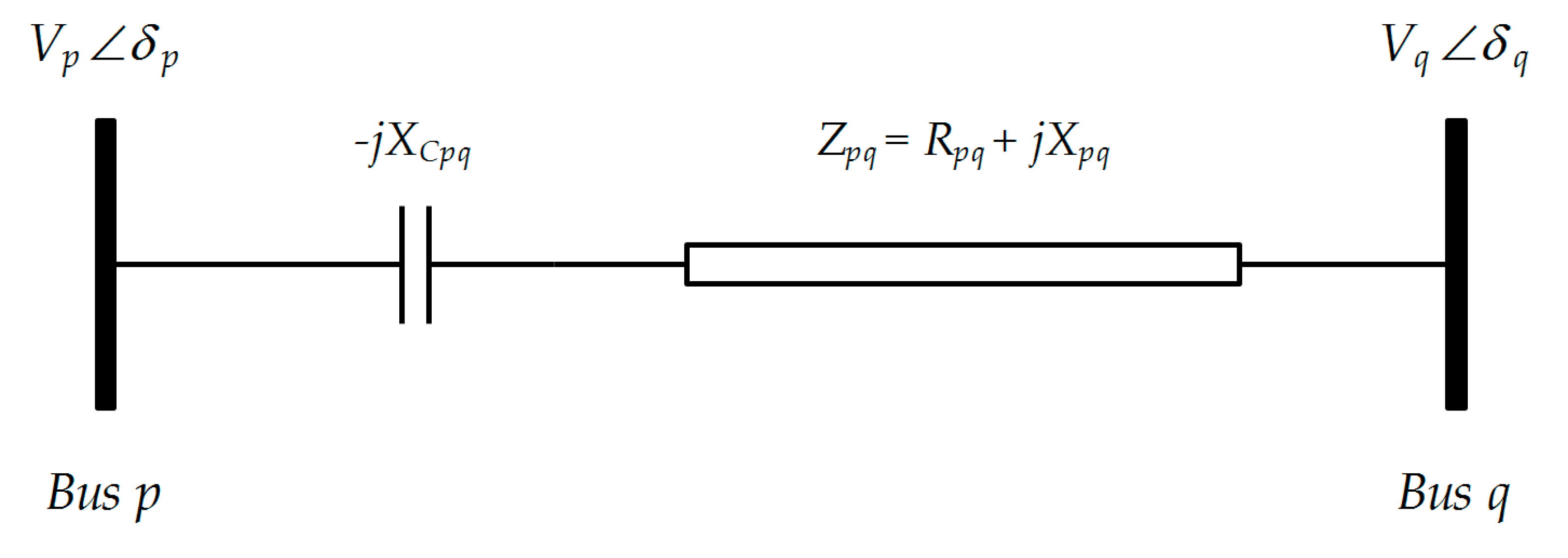
2.2. FACTS Devices Modeling

2.2.1. TCSC Modeling

Figure 1 shows the static of a TCSC connected between bus $p$ and $q$ [20,21].

The power flow equations from bus $p$ to bus $q$, including TCSC, are as follows [21]:

$$P_{pq}=V_p^2{G}_{pq}-V_p{V}_q{G}_{pq}\cos \left({\delta }_p-{\delta }_q\right)-V_p{V}_q{B}_{pq}\sin \left({\delta }_p-{\delta }_q\right)$$

(3)

$$Q_{pq}=-V_p^2{B}_{pq}-V_p{V}_q{G}_{pq}\sin \left({\delta }_p-{\delta }_q\right)+V_p{V}_q{B}_{pq}\cos \left({\delta }_p-{\delta }_q\right)$$

(4)

where

$$G_{pq}=\frac{R_{pq}}{R_{pq}^2+{(X_{pq}-X_{C_{pq}})}^2}$$

(5)

$$B_{pq}=\frac{R_{pq}}{R_{pq}^2+{(X_{pq}-X_{C_{pq}})}^2}$$

(6)

where $P_{pq}$ and $Q_{pq}$ are the active and reactive power flow from bus $p$ to bus $q$ with TCPS, respectively, $G_{pq}$ and $B_{pq}$ are the conductance and susceptance of transmission line between bus $p$ and bus $q$, respectively, ${\delta }_p$ and ${\delta }_q$ are the voltage angles at the $p^{th}$ bus and $q^{th}$ bus, respectively, $R_{pq}$ and $X_{pq}$ denote the resistance and reactance of the transmission line between bus $p$ and bus $q$, respectively, and lastly, $X_{C_{pq}}$ represents the reactance of the TCSC located in the transmission line between bus $p$ and bus $q$.

Similarity, the power flow equations from bus $q$ to bus $p$, including TCSC, are as follows:

$$P_{qp}=V_q^2{G}_{pq}-V_p{V}_q{G}_{pq}\cos \left({\delta }_p-{\delta }_q\right)+V_p{V}_q{B}_{pq}\sin \left({\delta }_p-{\delta }_q\right)$$

(7)

$$Q_{qp}=-V_q^2{B}_{pq}+V_p{V}_q{G}_{pq}\sin \left({\delta }_p-{\delta }_q\right)+V_p{V}_q{B}_{pq}\cos \left({\delta }_p-{\delta }_q\right)$$

(8)

where $P_{qp}$ and $Q_{qp}$ are the active and reactive power flow from bus $q$ to bus $p$ with TCPS, respectively.

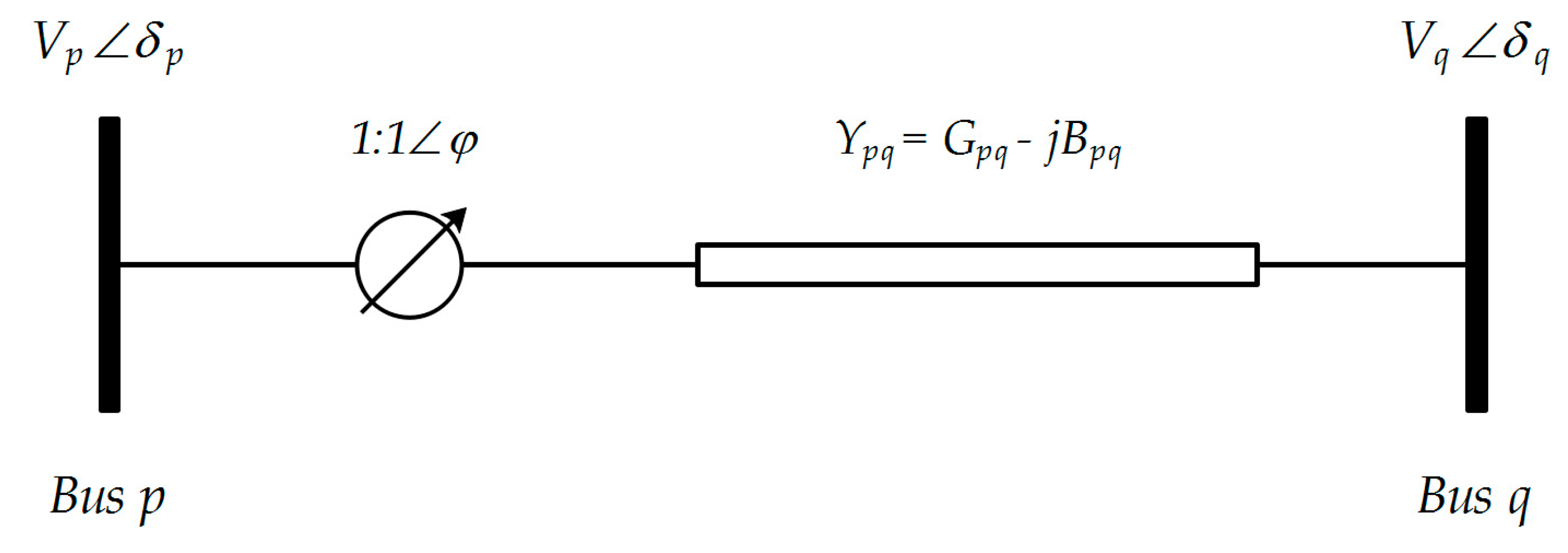
2.2.2. TCPS Modeling

Figure 2 demonstrates the static of a TCPS connected between bus $p$ and $q$, having a complex taping ratio of $1:1\angle \phi$ and series admittance of $Y_{pq}=G_{pq}-j{B}_{pq}$ [20].

The power flow equations from bus $p$ to bus $q$, including the TCPS, are as follows:

$$P_{pq}=\frac{V_p^2{G}_{pq}}{{\cos }^2\left(\phi \right)}-\frac{V_p{V}_q}{\cos \left(\phi \right)}\left[G_{pq}\cos \left({\delta }_p-{\delta }_q+\phi \right)+B_{pq}\sin \left({\delta }_p-{\delta }_q+\phi \right)\right]$$

(9)

$$Q_{pq}=-\frac{V_p^2{B}_{pq}}{{\cos }^2\left(\phi \right)}-\frac{V_p{V}_q}{\cos \left(\phi \right)}\left[G_{pq}\sin \left({\delta }_p-{\delta }_q+\phi \right)-B_{pq}\cos \left({\delta }_p-{\delta }_q+\phi \right)\right]$$

(10)

where $P_{pq}$ and $Q_{pq}$ are the active and reactive power flow from bus $p$ to bus $q$ with TCPS, respectively. In addition, $\phi$ shows the phase shift angle of TCPS.

Likewise, the power flow equations from bus $q$ to bus $p$, including the TCPS, are as follows:

$$P_{qp}=V_p^2{G}_{pq}-\frac{V_p{V}_q}{\cos \left(\phi \right)}\left[G_{pq}\cos \left({\delta }_p-{\delta }_q+\phi \right)-B_{pq}\sin \left({\delta }_p-{\delta }_q+\phi \right)\right]$$

(11)

$$Q_{qp}=-V_q^2{B}_{pq}+\frac{V_p{V}_q}{\cos \left(\phi \right)}\left[G_{pq}\sin \left({\delta }_p-{\delta }_q+\phi \right)+B_{pq}\cos \left({\delta }_p-{\delta }_q+\phi \right)\right]$$

(12)

where $P_{qp}$ and $Q_{qp}$ are the active and reactive power flow from bus $q$ to bus $p$ with TCPS, respectively.

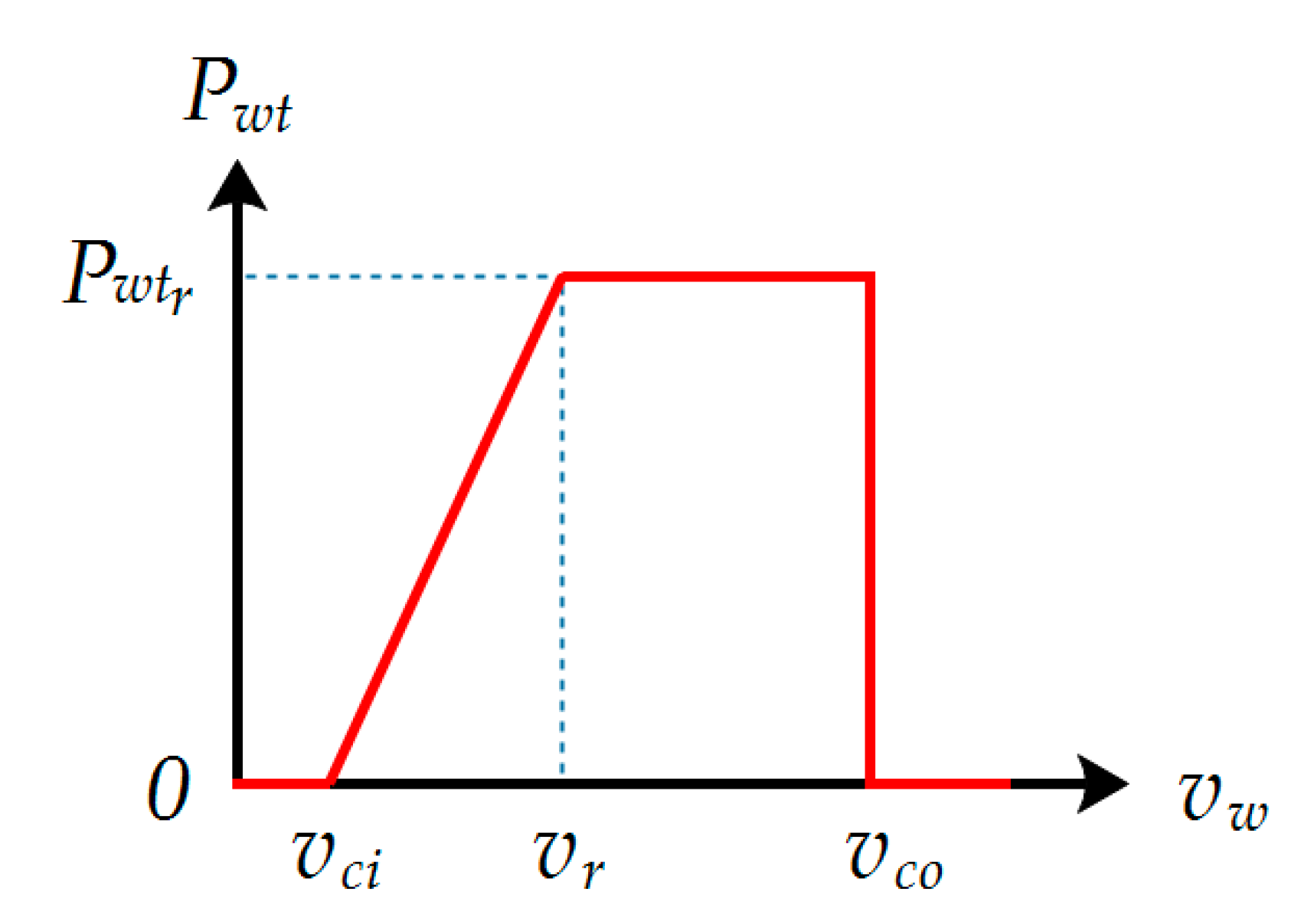
2.3. Wind Power Generation Modeling

The technology of wind turbines to generate electricity from wind can be divided into two major groups: (1) constant speed wind turbine, and (2) variable speed wind turbine. Fixed speed wind turbines are easy to install, more durable, and more affordable, while variable speed wind turbines should be installed according to the strategic and geographical conditions. Figure 3 shows the output power curve of a typical wind turbine. In Figure 3, $v_{ci}$ and $v_{ci}$ are the cut-in wind speed and cut-out wind speed, respectively, $v_r$ is the rated wind speed, and $v_w$ is the wind speed flowing into the wind turbine.

Since the wind speed is variable, the Weibull distribution is often considered as the probability density function that can be used to approximately model the behavior of the wind with a reasonable error. The Weibull distribution function to calculate the probability of the wind speed is as follows [22,23]:

$$f\left(v\right)=\left(\frac{k}{c}\right){\left(\frac{v}{c}\right)}^{k-1}{e}^{-{\left(\frac{v}{c}\right)}^k}$$

(13)

where $v$ shows the wind speed, and $k$ (shape factor) and $c$ (scale factor) are the wind speed parameters that vary depending on the region in which the wind blows.

It should be noted that to evaluate the power output of wind power, the problem has a general wind scenario, which initially generates a random number of wind speeds. Then, based on the Weibull distribution function considering the shape factor and scale factor, the probability of occurrence of those wind speeds is determined. Next, a certain number of wind speeds that most probably occur is selected. Finally, the average power of the wind farm is calculated.

2.4. Objective Functions

In this section, four different objective functions are presented.

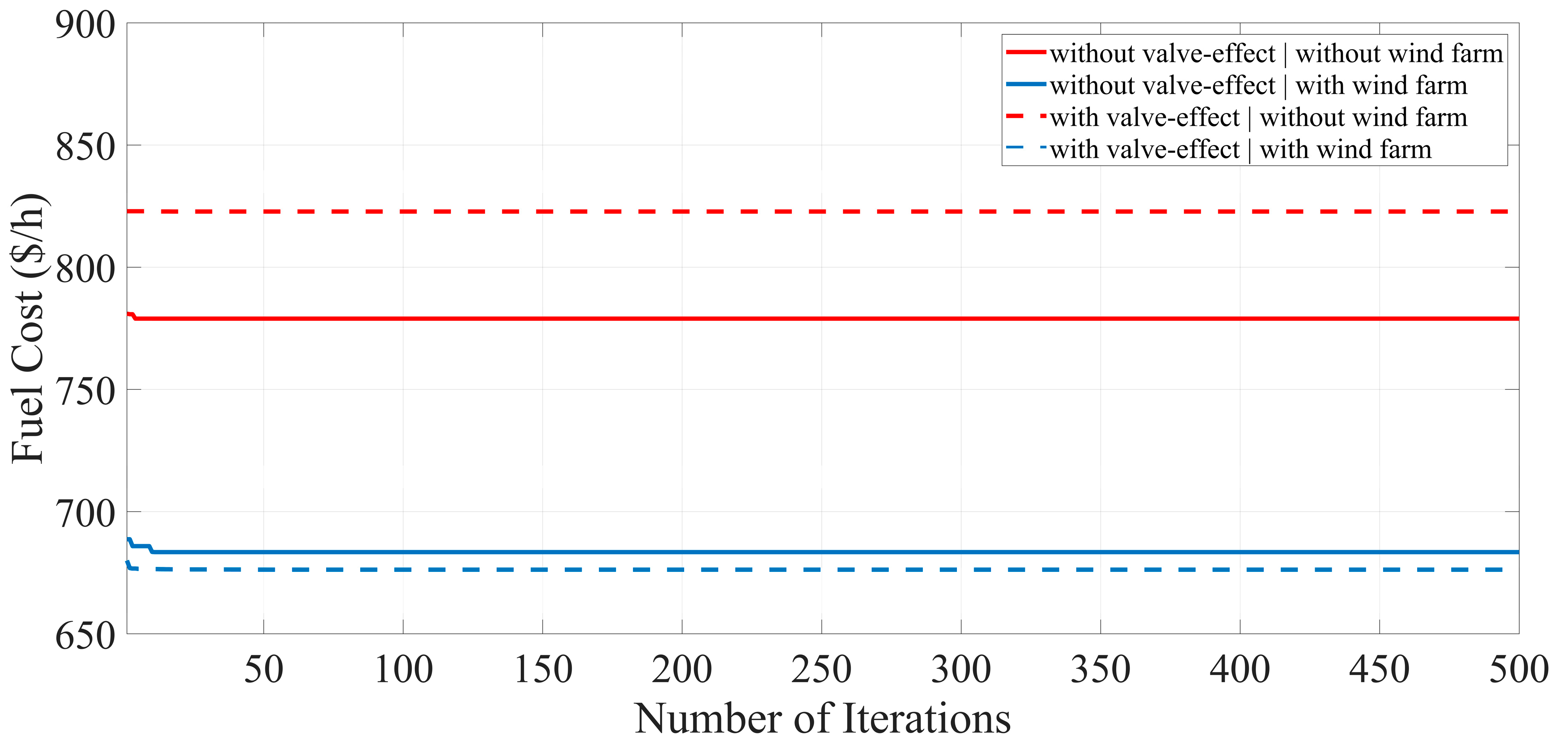
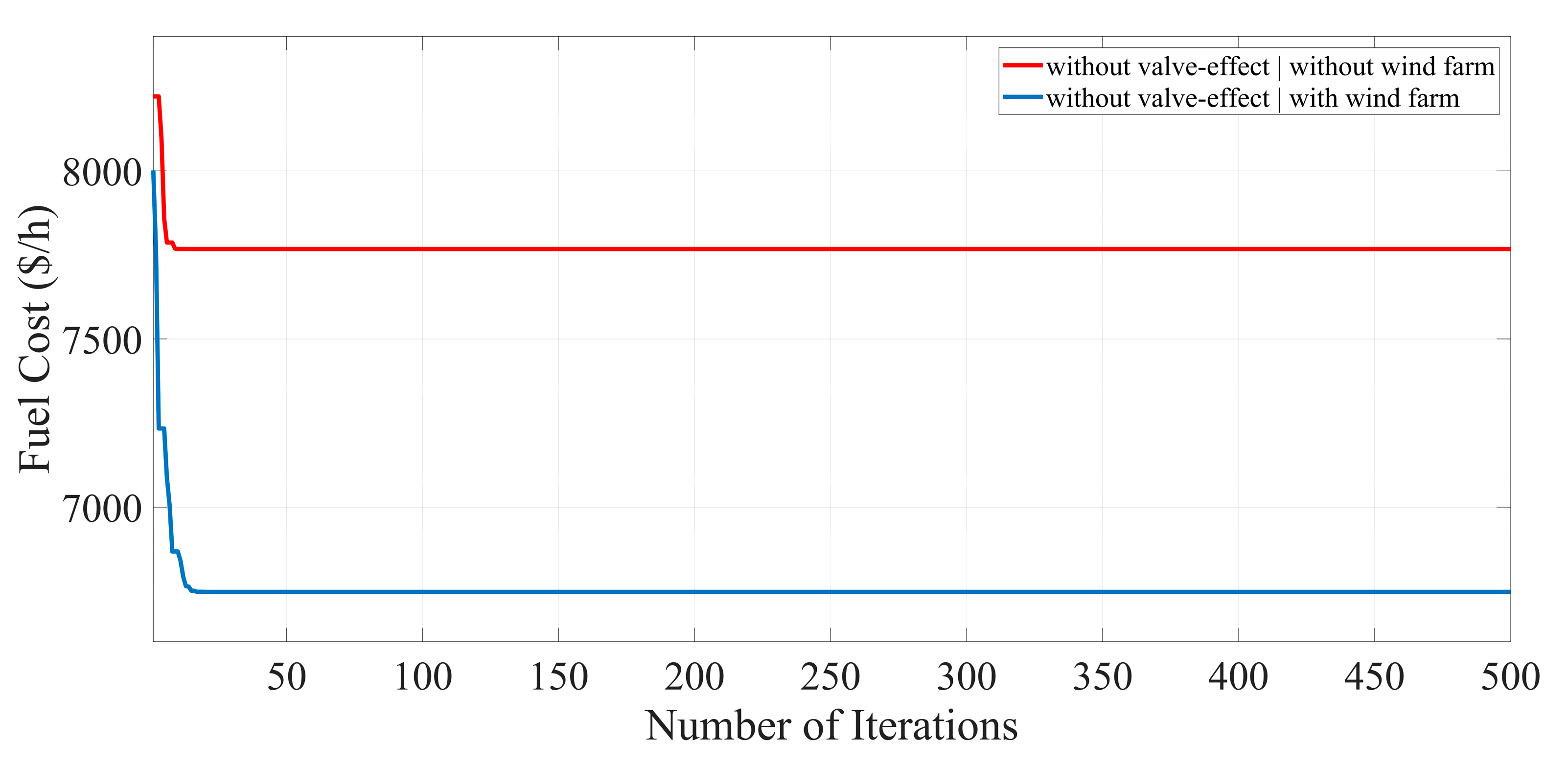
2.4.1. Minimization of Fuel Cost

Fuel cost minimization with a quadratic function is considered as the first objective function, as follows [24]:

$$\min F_C={\displaystyle \sum }_{p=1}^{N_{PV}}\left(a_p+b_p{P}_{G_p}+c_p{P}_{G_p}^2\right)$$

(14)

where $F_C$ is the total fuel cost of the generation units in ($/h), $a_p$, $b_p$, and $c_p$ are the fuel cost coefficients of the $p^{th}$ generation unit, $N_{PV}$ shows the total number of generation units, and $P_{G_p}$ denotes the generated active power by the $p^{th}$ generation unit.

Considering the valve-point effect, Equation (15) can be rewritten as follows:

$$\min F_C={\displaystyle \sum }_{p=1}^{N_{PV}}\left(a_p+b_p{P}_{G_p}+c_p{P}_{G_p}^2\right)+\left|d_p\sin \left(e_p\left(P_{G_p}^{min}-P_{G_p}\right)\right)\right|$$

(15)

where $d_p$ and $e_p$ are the fuel cost coefficients to model the valve-point effect, and $P_{G_p}^{min}$ denotes the minimum active power generated by the $p^{th}$ generation unit.

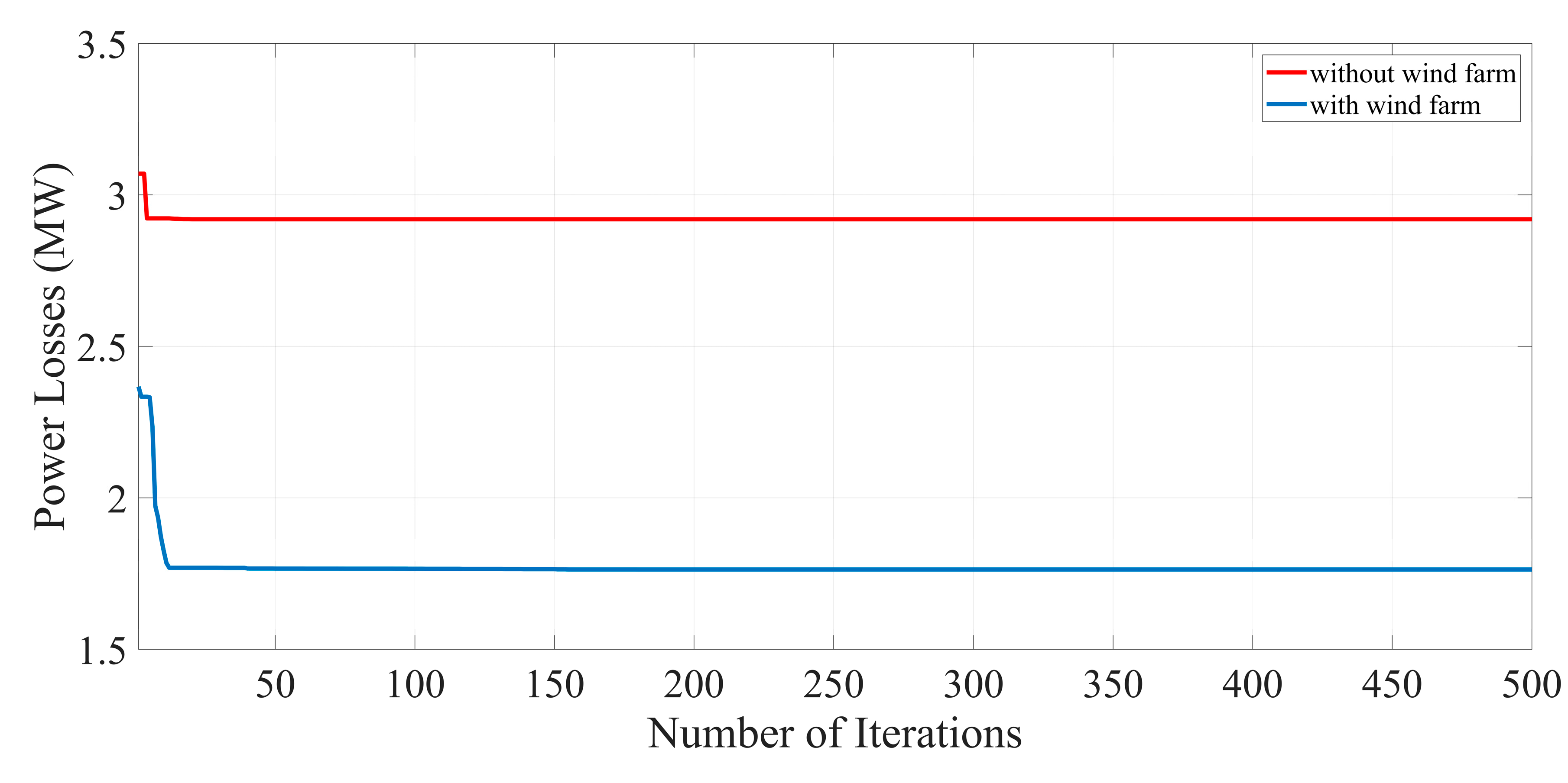
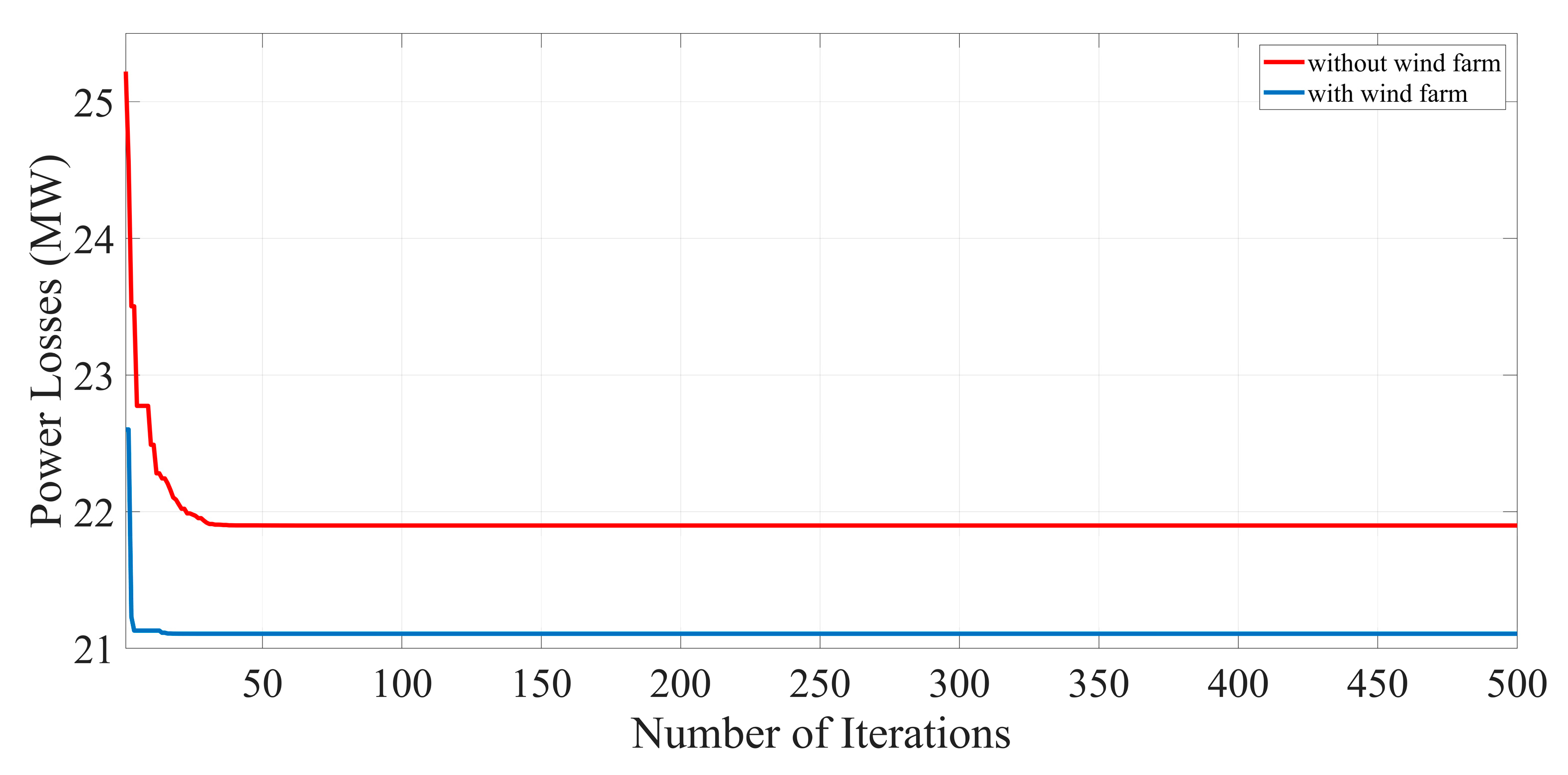
2.4.2. Minimization of Active Power Losses across the Transmission Lines

This objective function can be formulated as follows:

$$\min P_{Loss}={\displaystyle \sum }_{k=1}^{N_L}\left(G_k\left[V_p^2+V_q^2-2V_p{V}_q\cos \left({\delta }_p-{\delta }_q\right)\right]\right)$$

(16)

where $P_{Loss}$ is the total active power losses across the transmission lines in (MW), $G_k$ is the conductance of the $k^{th}$ transmission line connected between bus $p$ and bus $q$, $N_L$ is the total number of transmission lines, $V_p$ and $V_q$ are the voltage magnitudes of bus $p$ and bus $q$, respectively, and ${\delta }_p$ and ${\delta }_q$ are the voltage angles of bus $p$ and bus $q$, respectively.

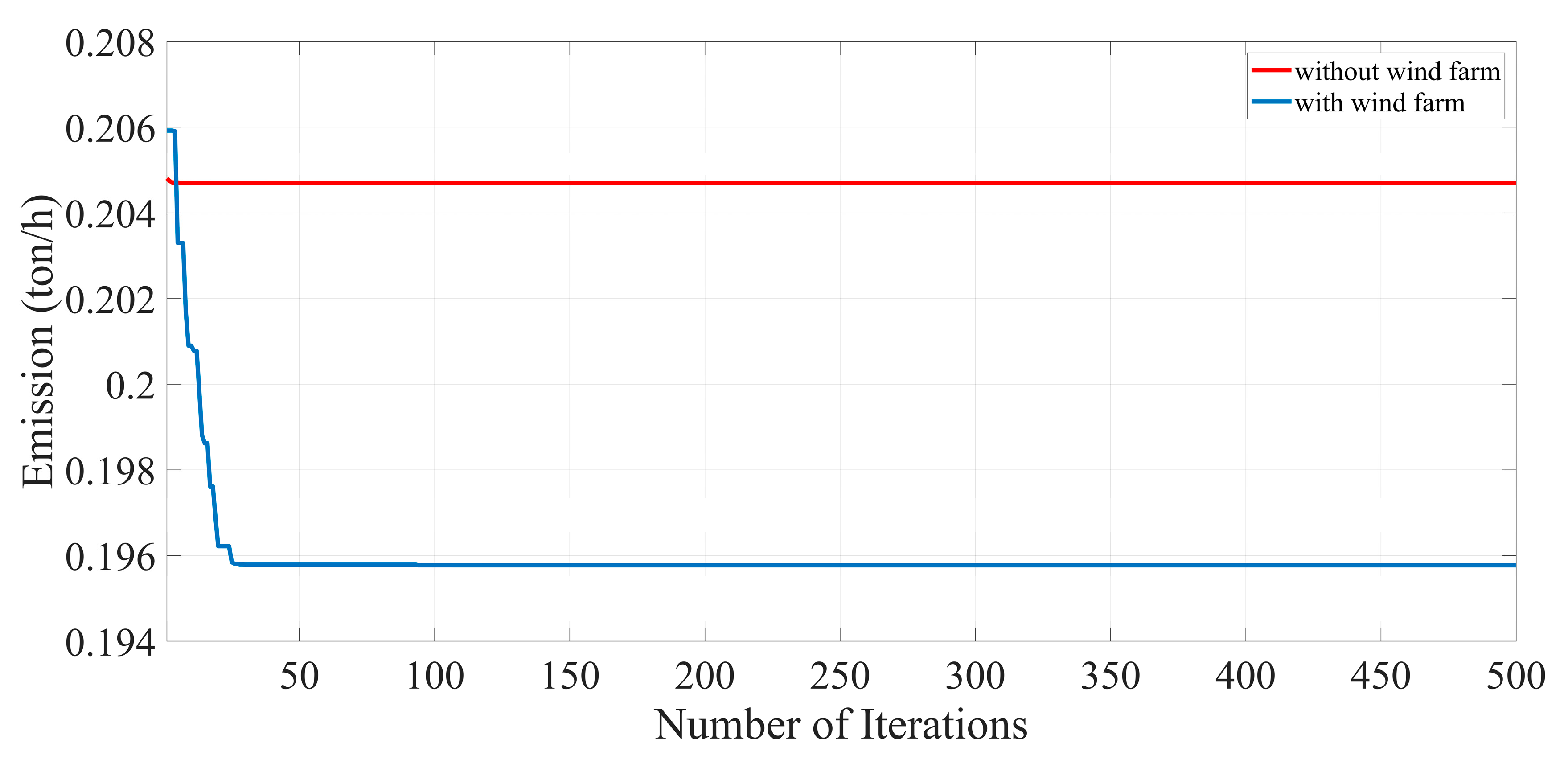
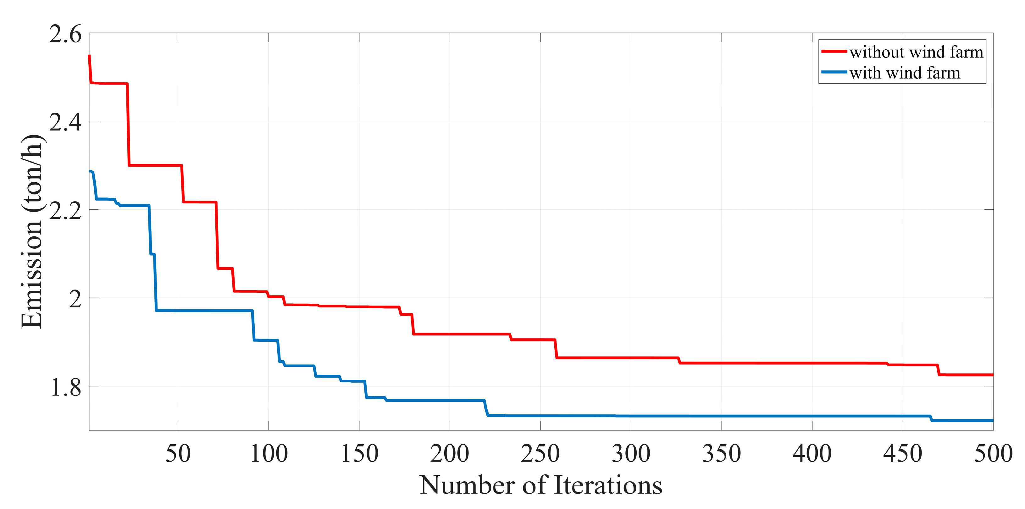
2.4.3. Minimization of Emission

The third objective function is to minimize the total emission, which is formulated as follows:

$$\min E\left(P_G\right)={\displaystyle \sum }_{k=1}^{N_{PV}}\left[{10}^{-2}\left({\alpha }_p+{\beta }_p{P}_{G_p}+{\gamma }_p{P}_{G_p}^2+{\eta }_p{e}^{{\lambda }_p{P}_{G_p}}\right)\right]$$

(17)

where $E\left(P_G\right)$ is the total emission due to the generation of the $p^{th}$ generation unit in (ton/h), and ${\alpha }_p$, ${\beta }_p$, ${\gamma }_p$, ${\eta }_p$, and ${\lambda }_p$ are the emission coefficients of the $p^{th}$ generation unit.

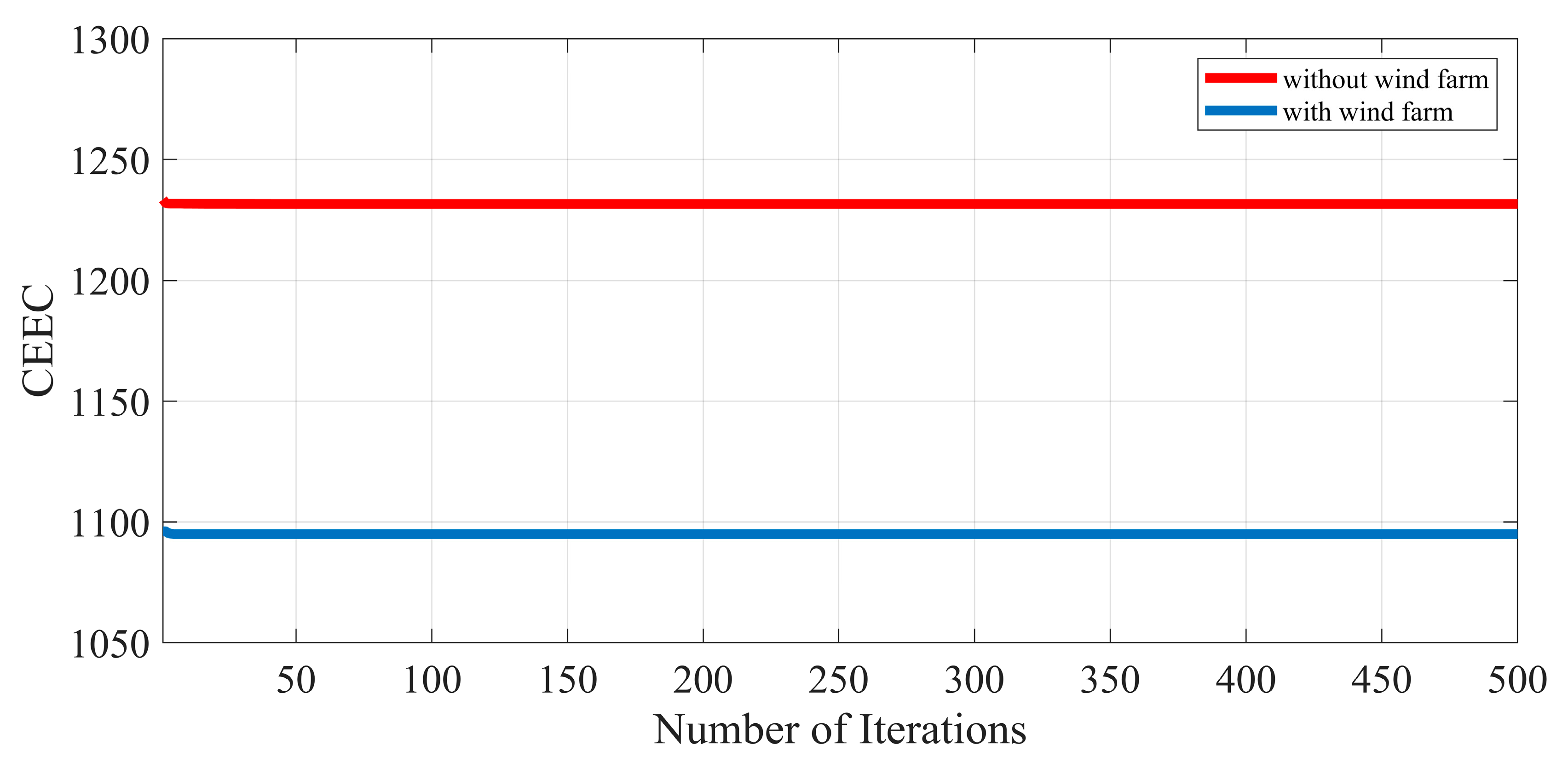
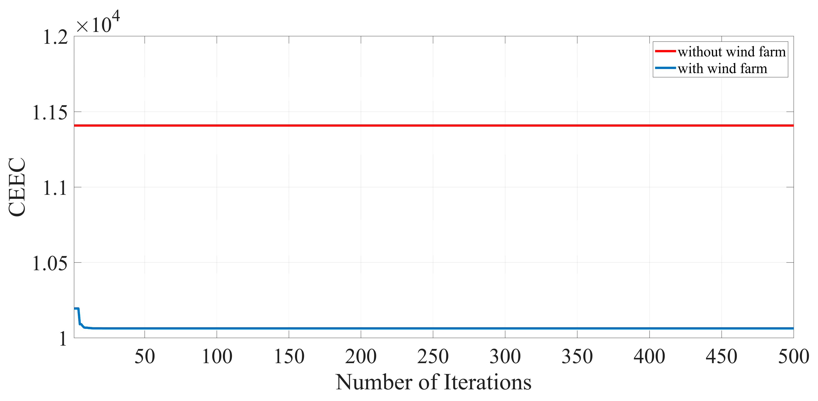
2.4.4. Minimization of the Combined Economic and Environmental Costs

The last objective function is to minimize the CEEC according to Equations (15) and (17):

$$\begin{gathered} \min CEEC=F_C+\mathsf{\Phi }.E\left(P_G\right) \\ ={\displaystyle \sum }_{p=1}^{N_{PV}}\left(a_p+b_p{P}_{G_p}+c_p{P}_{G_p}^2\right)+\left|d_p\sin \left(e_p\left(P_{G_p}^{min}-P_{G_p}\right)\right)\right|+\mathsf{\Phi }{\displaystyle \sum }_{k=1}^{N_{PV}}\left({\alpha }_p \\ +{\beta }_p{P}_{G_p}+{\gamma }_p{P}_{G_p}^2+{\eta }_p{e}^{{\lambda }_p{P}_{G_p}}\right) \end{gathered}$$

(18)

where $CEEC$ denotes the combined economic and environmental costs, and ${\mathsf{\Phi }}_p$ is the penalty factor, and can be obtained as follows:

$$\mathsf{\Phi }=\frac{a_p{\left(P_{G_p}^{max}\right)}^2+b_p{P}_{G_p}^{max}+c_p}{{\alpha }_p{\left(P_{G_p}^{max}\right)}^2+{\beta }_p{P}_{G_p}^{max}+{\gamma }_p}$$

(19)

The pollution charge coefficient for each unit is defined as the amount of fuel cost divided by the amount of pollution at its maximum output active power ($P_{G_p}^{max}$).

2.5. Constraints

In this section, different constraints are defined [24].

2.5.1. Load Flow Constraints

$$P_{wt}+{\displaystyle \sum }_{p=1}^{N_B}\left(P_{G_p}-P_{L_p}\right)+{\displaystyle \sum }_{p=1}^{N_{TPCS}}{P}_{pk}={\displaystyle \sum }_{p=1}^{N_B}{\displaystyle \sum }_{q=1}^{N_B}|V_p\left|\left|V_q\right|Y_{pq}\right|\cos \left({\theta }_{pq}+{\delta }_p-{\delta }_q\right)$$

(20)

$${\displaystyle \sum }_{p=1}^{N_B}\left(Q_{G_p}-P_{L_p}\right)+{\displaystyle \sum }_{p=1}^{N_{TPCS}}{Q}_{pk}=-{\displaystyle \sum }_{p=1}^{N_B}{\displaystyle \sum }_{q=1}^{N_B}|V_p\left|\left|V_q\right|Y_{pq}\right|\sin \left({\theta }_{pq}+{\delta }_p-{\delta }_q\right)$$

(21)

where $P_{G_p}$ and $Q_{G_p}$ are the generated active and reactive power at bus $p$, respectively, $P_{L_p}$ and $Q_{L_p}$ are the consumed active and reactive power at bus $p$, respectively, $P_{pk}$ and $Q_{pk}$ are the injected active and reactive power by the TCPSs at bus $p$, respectively, $P_{wt}$ indicates the generated active power by the wind turbine, $\left|Y_{pq}\right|$ and ${\theta }_{pq}$ are the magnitude and phase of the admittance of the transmission line between bus $p$ and bus $q$, $N_B$ shows the total number of buses, and $N_{TPCS}$ denotes the total number of TCPSs.

2.5.2. Active and Reactive Power of the Generation Units

$$P_{G_p}^{min}\le P_{G_p}\le P_{G_p}^{max}$$

(22)

$$Q_{G_p}^{min}\le Q_{G_p}\le Q_{G_p}^{max}$$

(23)

where for $p=1,\dots ,N_{PV}$ ($N_{PV}$ is the total number of generators), $P_{G_p}^{min}$ and $P_{G_p}^{max}$ are the minimum and maximum limits of the active power of the $p^{th}$ generator, respectively, and $Q_{G_p}^{min}$ and $Q_{G_p}^{max}$ are the minimum and maximum limits of the reactive power of the $p^{th}$ generator, respectively.

2.5.3. Voltage at Each Bus

$$V_{L_p}^{min}\le V_{L_p}\le V_{L_p}^{max}$$

(24)

where for $p=1,\dots ,N_{PQ}$ ($N_{PQ}$ is the total number of loads), $V_{L_p}^{min}$ and $V_{L_p}^{max}$ are the minimum and maximum level of the voltage at the $p^{th}$ load center, respectively.

2.5.4. Transformer Tap Settings

$$T_p^{min}\le T_p\le T_p^{max}$$

(25)

where for $p=1,\dots ,N_T$ ($N_T$ is the total number of transformers), $T_p^{min}$ and $T_p^{max}$ are the minimum and maximum tap settings limits of the $p^{th}$ transformer, respectively.

2.5.5. Transmission Lines Loading

$$S_{L_p}\le S_{L_p}^{max}$$

(26)

where for $p=1,\dots ,N_L$ ($N_L$ is the total number of transmission lines), $S_{L_p}$ and $S_{L_p}^{max}$ are the apparent power flow and maximum apparent power flow of the $p^{th}$ transmission line, respectively.

2.5.6. TCSC Reactance Constraints

$$X_{T_p}^{min}\le X_{T_p}\le X_{T_p}^{max}$$

(27)

where for $p=1,\dots ,N_{TCSC}$ ($N_{TCSC}$ is the total number of TCSCs), $X_{T_p}^{min}$ and $X_{T_p}^{max}$ are the minimum and maximum reactance of the $p^{th}$ TCSC, respectively.

2.5.7. TCPS Phase Shift

$${\phi }_{T_p}^{min}\le {\phi }_{T_p}\le {\phi }_{T_p}^{max}$$

(28)

where for $p=1,\dots ,N_{TCPS}$ ($N_{TCPS}$ is the total number of TCPSs), ${\phi }_{T_p}^{min}$ and ${\phi }_{T_p}^{max}$ are the minimum and maximum phase shift angle of the $p^{th}$ TCPS, respectively.

2.6. Solution Method

The KHA is based on the herding behavior of krill swarms in response to the specific biological and environmental processes [25]. In this paper, the KHA is used to solve the OPF problem incorporating stochastic wind power generation and FACTS devices considering uncertainty. The followings are the steps to implement the KHA.

Step 1:

Start

Step 2:

Check the data structure

Step 3:

Initialization

Step 4:

Fitness evaluation and check for constraints

Step 5:

Motion calculation

  Induced motion

  Foraging motion

  Physical diffusion

Step 6:

Implementation of the genetic operator

Step 7:

Check the results based on updating the krill individual position in the search space

Step 8:

If the best results are achieved then

   Go to Step 9

   Otherwise

   Go to Step 4

Step 9:

End

3. Simulation Results

To demonstrate the applicability and validity of the proposed method, two different test systems, (1) IEEE 30-bus test system, and (2) IEEE 57-bus test system are analyzed [26,27]. In addition, a wind farm consisting of 20 × 2 MW wind turbines is considered. It should be noted that the number of iterations for all simulated cases is set to 500. The highlighted rows in all tables show the corresponding values for the specific objective functions.

3.1. Case 1: IEEE 30-Bus Test System

The IEEE 30-bus test system consists of 21 load centers with an overall power consumption of 4283 MW. It has six generators at buses 1, 2, 5, 8, 11, and 13. Totally, nine reactive power control devices are located at buses 10, 12, 15, 17, 20, 21, 23, 24, and 29. In addition, the range of voltage in this case study is considered between 0.95 and 1.05 p.u. There are 41 transmission lines. The tap changers are located in transmission lines 6–9, 6–10, 4–12, and 28–27. According to [13], two TCSCs are installed in transmission lines 3–4, 19–20 with 50% (minimum) and 100% (maximum) series line reactances, and two TCPS are also placed on transmission lines 5–7 and 10–22 with –5° (minimum) and +5° (maximum) phase shift angles. In addition, the wind farm is placed on bus 22 [27]. In this section, two case studies, considering the wind farm in power systems and neglecting it are carried out.

3.1.1. Minimization of Fuel Cost

The simulation results without considering the valve-point effect, with and without wind farm (as indicated by $P_{wind}$), are provided in

Table 3. Results for fuel cost minimization without considering the valve-point effect for the Test System 1.

Control Variable	Without Wind Farm				With Wind Farm
	KHA	ALC-PSO	DEA	RCGA	KHA
$P_{G_1}$ (MW)	179.755	185.240	180.260	192.460	137.526
$P_{G_2}$ (MW)	47.8185	46.3300	49.3200	48.3800	41.9122
$P_{G_5}$ (MW)	18.5154	20.8800	20.8200	19.5400	19.3311
$P_{G_8}$ (MW)	16.0965	15.6400	17.6100	11.6000	15.5927
$P_{G_{11}}$ (MW)	10.0000	11.1200	11.0500	10.0000	20.9936
$P_{G_{13}}$ (MW)	19.3238	12.5800	12.6900	12.0000	17.7110
Total Generation (MW)	291.509	291.790	291.750	294.000	253.067
$P_{wind}$ (MW)	0.00000	0.00000	0.00000	0.00000	34.4126
Fuel Cost ($/h)	779.393	796.930	797.290	803.840	683.646
Emission (ton/h)	0.42496	0.39020	0.37560	0.00000	0.28904
Power Losses (MW)	8.10960	8.39000	8.35000	10.6000	4.08011
Computation Time (s)	184.400	479.200	487.300	265.800	188.100

. The simulation results considering the valve-point effect, with and without wind farm, are also given in

Table 4. Results for fuel cost minimization considering the valve-point effect for the Test System 1.

Control Variable	Without Wind Farm				With Wind Farm
	KHA	ALC-PSO	DEA	RCGA	KHA
$P_{G_1}$ (MW)	191.690	199.850	199.130	198.810	130.246
$P_{G_2}$ (MW)	34.4058	38.2000	38.3200	38.9600	39.4530
$P_{G_5}$ (MW)	15.0000	20.1600	20.1700	19.1600	32.9689
$P_{G_8}$ (MW)	10.0000	11.1500	11.4300	10.6400	29.5335
$P_{G_{11}}$ (MW)	19.2954	10.1300	10.4300	13.5600	11.8032
$P_{G_{13}}$ (MW)	21.0191	12.6600	12.6600	12.0300	12.0000
Total Generation (MW)	291.410	292.150	292.140	293.160	256.005
$P_{wind}$ (MW)	0.00000	0.00000	0.00000	0.00000	32.6020
Fuel Cost ($/h)	824.150	825.890	826.540	831.030	676.762
Emission (ton/h)	0.44373	0.44124	0.43830	0.43660	0.30525
Power Losses (MW)	8.01050	8.75000	8.74000	9.76000	5.20730
Computation Time (s)	185.700	503.120	505.600	714.800	189.000

. Table 3 and Table 4 show that the presence of a wind farm in the case study reduces the generation capacity of other generation units and decreases the fuel costs and emission. Additionally, the results of Particle Swarm Optimization with Aging Leader and Challengers (ALC-PSO), DEA, and Real-Coded Genetic Algorithm (RCGA) are presented to evaluate and compare the performance and accuracy of KHA [28].

According to the obtained results, the values of objective function without considering the valve-point effect and without wind farm using ALC-PSO, DEA, and RCGA are 17.537, 17.897, and 24.447 $/h more than KHA, respectively. Considering such conditions in the presence of the wind farm, the value of the objective function using KHA is 683.646 $/h, which is 95.747 $/h less than the case without the wind farm.

In addition, the values of objective function considering the valve-point effect and with wind farm using ALC-PSO, DEA, and RCGA are 1.74, 2.39, and 6.88 $/h more than KHA, respectively. Considering such conditions in the presence of the wind farm, the value of the objective function using KHA is 676.762 $/h, which is 147.388 $/h less than the case without the wind farm.

3.1.2. Minimization of Active Power Losses across the Transmission Lines

Table 5. Results for minimizing the active power losses across the transmission lines for the Test System 1.

Control Variable	Without Wind Farm				With Wind Farm
	KHA	ALC-PSO	DEA	RCGA	KHA
$P_{G_1}$ (MW)	98.0937	74.6900	77.5900	77.5800	15.7459
$P_{G_2}$ (MW)	53.5641	67.3000	67.3000	69.5800	80.0000
$P_{G_5}$ (MW)	50.0000	50.0000	50.0000	49.9800	50.0000
$P_{G_8}$ (MW)	35.0000	34.6600	34.8500	34.9600	35.0000
$P_{G_{11}}$ (MW)	16.5549	27.2600	27.0400	23.6900	30.0000
$P_{G_{13}}$ (MW)	32.8586	32.2200	32.3600	30.4300	40.0000
Total Generation (MW)	286.071	286.130	285.140	286.220	250.745
$P_{wind}$ (MW)	0.00000	0.00000	0.00000	0.00000	34.4212
Fuel Cost ($/h)	992.050	992.180	992.300	985.210	918.639
Emission (ton/h)	0.21091	0.21090	0.21090	0.21440	0.21031
Power Losses (MW)	2.92130	2.98000	2.99000	3.07000	1.76710
Computation Time (s)	170.150	482.100	497.400	711.700	174.300

shows the best control variable settings for the minimization of the active power losses across the transmission lines of the IEEE 30-bus test system using KHA. According to Table 5, the presence of a wind farm in power systems reduces the active power losses across the transmission lines.

As shown in Table 5, the values of objective function without wind farm using ALC-PSO, DEA, and RCGA are 0.0587, 0.0687, and 0.1487 MW more than KHA, respectively. Considering such conditions in the presence of the wind farm, the value of the objective function using KHA is 1.76710 MW, which is 1.1542 MW less than the case without the wind farm.

3.1.3. Minimization of Active Power Losses across the Transmission Lines

Table 6. Results for emission minimization for the Test System 1.

Control Variable	Without Wind Farm				With Wind Farm
	KHA	ALC-PSO	DEA	RCGA	KHA
$P_{G_1}$ (MW)	51.3924	64.5200	63.5000	63.9800	45.9204
$P_{G_2}$ (MW)	80.0000	66.9000	67.9200	67.7500	51.6969
$P_{G_5}$ (MW)	50.0000	50.0000	50.0000	50.0000	50.0000
$P_{G_8}$ (MW)	35.0000	35.0000	35.0000	35.0000	35.0000
$P_{G_{11}}$ (MW)	30.0000	30.0000	30.0000	29.9600	30.0000
$P_{G_{13}}$ (MW)	40.0000	40.0000	40.0000	40.0000	40.0000
Total Generation (MW)	286.392	286.420	286.420	286.690	252.617
$P_{wind}$ (MW)	0.00000	0.00000	0.00000	0.00000	33.3285
Fuel Cost ($/h)	1012.75	1014.24	1015.10	1015.80	906.068
Emission (ton/h)	0.20469	0.20475	0.20480	0.20490	0.19587
Power Losses (MW)	2.99240	3.02000	3.02000	3.29000	2.54580
Computation Time (s)	169.140	506.100	511.300	706.000	173.180

shows the best control variable settings for the emission minimization of the IEEE 30-bus test systems using KHA. Table 6 shows that the presence of a wind farm in power systems decreases the emission.

According to the obtained results, the values of objective function without wind farm using ALC-PSO, DEA, and RCGA are 0.00006, 0.00011, and 0.00021 ton/h more than KHA, respectively. Considering such conditions in the presence of the wind farm, the value of the objective function using KHA is 0.19587 ton/h, which is 0.00882 ton/h less than the case without the wind farm.

3.1.4. Minimization of Combined Economic and Environmental Costs

Table 7. Results for emission minimization for the Test System 1.

Control Variable	Without Wind Farm			With Wind Farm
	KHA	ALC-PSO	DEA	KHA
$P_{G_1}$ (MW)	126.476	115.230	107.980	110.376
$P_{G_2}$ (MW)	66.4293	56.5700	58.5700	63.8014
$P_{G_5}$ (MW)	29.8519	31.8800	32.3800	23.7588
$P_{G_8}$ (MW)	27.9298	27.5400	27.6100	17.1252
$P_{G_{11}}$ (MW)	18.0473	23.8900	29.5100	16.7590
$P_{G_{13}}$ (MW)	19.8514	34.2300	33.2700	23.6716
Total Generation (MW)	288.585	289.330	289.320	255.492
$P_{wind}$ (MW)	0.00000	0.00000	0.00000	32.3655
Fuel Cost ($/h)	897.430	907.170	922.360	784.653
Emission (ton/h)	0.23990	0.24302	0.23640	0.22423
Power Losses (MW)	5.18590	5.92000	5.93000	4.45820
CEEC	1232.80	1234.44	1238.09	1095.72
Computation Time (s)	189.140	515.100	521.300	189.180

demonstrates the best control variable settings for the CEEC minimization of the IEEE 30-bus test systems using KHA. According to the obtained results, the presence of a wind farm in power systems decreases the CEEC.

As shown in Table 7, the values of objective function without wind farm using ALC-PSO and DEA are 1.64 and 5.29 more than KHA, respectively. Considering such conditions in the presence of the wind farm, the value of the objective function using KHA is 1095.72, which is 137.08 less than the case without the wind farm.

Figure 4, Figure 5, Figure 6 and Figure 7 show the convergence curves of the defined objective functions for the Test System 1 after 500 iterations.

3.2. Case 2: IEEE 57-Bus Test System

The IEEE 57-bus test system, which consists of 7 generators located at the buses 1, 2, 3, 6, 8, 9, and 12 with 15 transformers under load tap settings, is chosen as test system 2. Three reactive power sources are taken at buses 18, 25, and 53. In this paper, TCSCs are located in transmission lines 18–19, 31–32, 34–32, 40–56, and 39–57. TCPSs are also installed in transmission lines 4–5, 5–6, 26–27, 41–43, and 53–54. The wind farm is placed at bus 52 [27]. The same as the previous section, two case studies, considering the wind farm in power systems and neglecting it, are carried out.

Table 8. Results for fuel cost minimization without considering the valve-point effect for the Test System 2.

Control Variable	Without Wind Farm				With Wind Farm
	KHA	ALC-PSO	DEA	RCGA	KHA
$P_{G_1}$ (MW)	584.6750	514.2600	520.0900	517.4500	422.6630
$P_{G_2}$ (MW)	0.000000	0.000000	0.000000	0.000000	105.4910
$P_{G_5}$ (MW)	75.16610	123.5300	103.7400	94.81000	161.5274
$P_{G_6}$ (MW)	0.000000	0.000000	0.000000	0.000000	182.3932
$P_{G_8}$ (MW)	166.0264	159.6700	175.6300	181.7500	0.00000
$P_{G_9}$ (MW)	253.7019	0.000000	0.000000	0.000000	125.9095
$P_{G_{12}}$ (MW)	211.8802	486.8900	485.2300	489.7700	256.8480
Total Generation (MW)	1291.449	1284.350	1284.690	1283.780	1254.832
$P_{wind}$ (MW)	0.000000	0.000000	0.000000	0.000000	36.37860
Fuel Cost ($/h)	7768.000	8103.180	8309.270	8413.430	6748.000
Emission (ton/h)	2.379500	2.397820	2.433300	2.433100	2.018000
Power Losses (MW)	40.64980	33.55000	33.89000	32.98000	40.41060
Computation Time (s)	678.9000	680.1200	689.9000	847.9000	714.7000

,

Table 9. Results for minimizing the active power losses across the transmission lines for the Test System 2.

Control Variable	Without Wind Farm				With Wind Farm
	KHA	ALC-PSO	DEA	RCGA	KHA
$P_{G_1}$ (MW)	192.3159	303.2400	318.5800	311.3400	176.1450
$P_{G_2}$ (MW)	0.000000	0.000000	0.000000	0.000000	16.85120
$P_{G_5}$ (MW)	34.34410	63.19000	45.90000	60.61300	156.9747
$P_{G_6}$ (MW)	134.0298	0.000000	0.000000	0.000000	58.62480
$P_{G_8}$ (MW)	469.7929	400.7500	407.6500	400.0600	158.5790
$P_{G_9}$ (MW)	0.000000	0.000000	0.000000	0.000000	290.1441
$P_{G_{12}}$ (MW)	436.1565	500.0000	495.0300	495.1400	371.8631
Total Generation (MW)	1266.639	1267.180	1267.160	1267.153	1229.181
$P_{wind}$ (MW)	0.000000	0.000000	0.000000	0.000000	35.46800
Fuel Cost ($/h)	15,354.40	15,423.88	15,691.30	15,348.11	13,078.79
Emission (ton/h)	1.916836	1.906545	1.966905	1.917299	1.507600
Power Losses (MW)	21.93910	22.48000	22.46000	22.46300	21.11000
Computation Time (s)	670.2000	881.3000	701.7000	691.0450	715.0000

,

Table 10. Results for minimizing the active power losses across the transmission lines for the Test System 2.

Control Variable	Without Wind Farm				With Wind Farm
	KHA	ALC-PSO	DEA	RCGA	KHA
$P_{G_1}$ (MW)	333.585	341.910	298.12	300.23	143.311
$P_{G_2}$ (MW)	0.00000	0.00000	0.00000	0.00000	149.200
$P_{G_5}$ (MW)	170.617	91.9000	83.24	91.43	158.020
$P_{G_6}$ (MW)	0.00000	0.00000	0.00000	0.00000	161.346
$P_{G_8}$ (MW)	311.707	419.250	413.63	406.26	220.977
$P_{G_9}$ (MW)	0.00000	0.00000	0.00000	0.00000	173.139
$P_{G_{12}}$ (MW)	453.292	418.450	474.14	472.08	228.994
Total Generation (MW)	1269.20	1271.51	1269.13	1270	1234.99
$P_{wind}$ (MW)	0.00000	0.00000	0.00000	0.00000	34.2539
Fuel Cost ($/h)	15,667.9	15,856.1	15,914.3	15,577.3	15,202.6
Emission (ton/h)	1.82129	1.88918	1.85870	1.83871	1.72090
Power Losses (MW)	18.4031	20.7100	18.3300	19.2000	18.4442
Computation Time (s)	690.100	878.700	694.200	690.140	705.510

and

Table 11. Results for CEEC minimization for the Test System 2.

Control Variable	Without Wind Farm			With Wind Farm
	KHA	ALC-PSO	DEA	KHA
$P_{G_1}$ (MW)	346.8868	480.9300	475.6800	92.82350
$P_{G_2}$ (MW)	0.000000	0.000000	0.000000	286.8995
$P_{G_5}$ (MW)	173.0854	80.14000	80.64000	89.87540
$P_{G_6}$ (MW)	0.000000	0.000000	0.000000	193.2463
$P_{G_8}$ (MW)	157.0796	270.4200	276.0300	13.55130
$P_{G_9}$ (MW)	0.000000	0.000000	0.000000	89.01440
$P_{G_{12}}$ (MW)	583.2398	446.0400	447.2000	459.5085
Total Generation (MW)	1260.291	1279.530	1279.550	1224.918
$P_{wind}$ (MW)	0.000000	0.000000	0.000000	36.18200
Fuel Cost ($/h)	9917.870	10,237.79	10,408.49	8481.851
Emission (ton/h)	2.200089	2.227447	2.211635	1.620300
Power Losses (MW)	9.491500	28.73000	28.75000	10.30090
CEEC	11,410.00	13,032.56	13,183.42	10,060.00
Computation Time (s)	690.1000	700.1400	702.2000	717.5100

show the best control variable settings for different objective functions of the IEEE 57-bus test system using KHA.

According to the obtained results from Table 8, Table 9, Table 10 and Table 11, considering wind farm in power system cause a significant reduction on power losses across the transmission lines, emission, and CEEC.

In addition, Figure 8, Figure 9, Figure 10 and Figure 11 show the convergence curves of the defined objective functions for the Test System 2 after 500 iterations.

4. Conclusions

A new meta-heuristic algorithm is proposed in this paper to cope with the Optimal Power Flow (OPF) problem of power systems incorporated with wind farm and FACTS devices. Four different objective functions, including minimization of fuel cost, minimization of power losses across the transmission line, emission reduction, and combined economic and environmental cost minimization are formulated separately in this paper. To show the effectiveness of the proposed approach, the IEEE 30-bus test system and the IEEE 57-bus test system with the installation of thyristor controlled phase shifter (TCPS) and thyristor-controlled series compensator (TCSC) and a wind farm are simulated. Based on numerical results, it is observed that the krill herd algorithm (KHA) has great capability to achieve an optimal solution in the target functions with less computation time. The proposed method indicates an improved convergence performance to optimal solutions than other heuristic techniques and can be applied to cope with complex optimization problems in modern power systems. It can efficiently deal with the uncertainties in wind power generation. In addition, it is shown that the presence of the wind farm in power systems minimizes the d the generation capacity of the other generating unit, which reduces the dependency on conventional power plants, thus, reducing power losses across the transmission lines and reducing emission as well as the combined economic and environmental costs (CEEC).

References

1. Kahourzade, S.; Mahmoudi, A.; Mokhlis, H.B. A Comparative Study of Multi-Objective Optimal Power Flow Based on Particle Swarm, Evolutionary Programming, and Genetic Algorithm. Electr. Eng. 2015, 97, 1–12. [Google Scholar] [CrossRef] [Green Version]
2. Viafora, N.; Delikaraoglou, S.; Pinson, P.; Holbøll, J. Chance-Constrained Optimal Power Flow with Non-Parametric Probability Distributions of Dynamic Line Ratings. Int. J. Electr. Power Energy Syst. 2020, 114, 105389. [Google Scholar] [CrossRef]
3. Dong, X.; Zhang, R.; Wang, M.; Wang, J.; Wang, C.; Wang, Y.; Wang, P. Capacity Assessment for Wind Power Integration Considering Transmission Line Electro-Thermal Inertia. Int. J. Electr. Power Energy Syst. 2020, 118, 105724. [Google Scholar] [CrossRef]
4. Miveh, M.R.; Rahmat, M.F.; Ghadimi, A.A.; Mustafa, M.W. Control Techniques for Three-Phase Four-Leg Voltage Source Inverters in Autonomous Microgrids: A Review. Renew. Sustain. Energy Rev. 2016, 54, 1592–1610. [Google Scholar] [CrossRef]
5. Heideier, R.; Bajay, S.V.; Jannuzzi, G.M.; Gomes, R.D.M.; Guanais, L.; Ribeiro, I.; Paccola, A. Impacts of Photovoltaic Distributed Generation and Energy Efficiency Measures on the Electricity Market of Three Representative Brazilian Distribution Utilities. Energy Sustain. Dev. 2020, 54, 60–71. [Google Scholar] [CrossRef]
6. Zhang, Y.; Yao, F.; Iu, H.H.-C.; Fernando, T.; Wong, K.P. Sequential Quadratic Programming Particle Swarm Optimization for Wind Power System Operations Considering Emissions. J. Mod. Power Syst. Clean Energy 2013, 1, 231–240. [Google Scholar] [CrossRef] [Green Version]
7. Baskaran, J.; Palanisamy, V. Optimal Location of FACTS Devices in a Power System Solved by a Hybrid Approach. Nonlinear Anal. Theory Methods Appl. 2006, 65, 2094–2102. [Google Scholar] [CrossRef]
8. Roy, R.; Jadhav, H.T. Optimal Power Flow Solution of Power System Incorporating Stochastic Wind Power Using Gbest Guided Artificial Bee Colony Algorithm. Int. J. Electr. Power Energy Syst. 2015, 64, 562–578. [Google Scholar] [CrossRef]
9. Gotham, D.J.; Heydt, G.T. Power Flow Control and Power Flow Studies for Systems with FACTS Devices. IEEE Trans. Power Syst. 1998, 13, 60–65. [Google Scholar] [CrossRef]
10. Bhattacharyya, B.; Gupta, V.K.; Kumar, S. UPFC with Series and Shunt FACTS Controllers for the Economic Operation of a Power System. Ain Shams Eng. J. 2014, 5, 775–787. [Google Scholar] [CrossRef]
11. Noroozian, M.; Angquist, L.; Ghandhari, M.; Andersson, G. Use of UPFC for Optimal Power Flow Control. IEEE Trans. Power Deliv. 1997, 12, 1629–1634. [Google Scholar] [CrossRef]
12. Behshad, M.; Lashkarara, A.; Rahmani, A.H. Optimal Location of UPFC Device Considering System Loadability, Total Fuel Cost, Power Losses and Cost of Installation. In Proceedings of the 2nd International Conference on Power Electronics and Intelligent Transportation System, Shenzhen, China, 19–20 December 2009. [Google Scholar]
13. Basu, M. Multi-Objective Optimal Power Flow with FACTS Devices. Energy Convers. Manag. 2011, 52, 903–910. [Google Scholar] [CrossRef]
14. Pattanaik, J.K.; Basu, M.; Dash, D.P. Optimal Power Flow with FACTS Devices Using Artificial Immune Systems. In Proceedings of the International Conference on Technological Advancements in Power and Energy, Kollam, India, 21–23 December 2017. [Google Scholar]
15. Vanitha, R.; Baskaran, J.; Sudhakaran, M. Multi Objective Optimal Power Flow with STATCOM Using DE in WAFGP. Indian J. Sci. Technol. 2015, 8, 191. [Google Scholar] [CrossRef]
16. Ongsakul, W.; Bhasaputra, P. Optimal Power Flow with FACTS Devices by Hybrid TS/SA Approach. Int. J. Electr. Power Energy Syst. 2002, 24, 851–857. [Google Scholar] [CrossRef]
17. Leung, H.C.; Chung, T.S. Optimal Power Flow with a Versatile FACTS Controller by Genetic Algorithm Approach. In Proceedings of the 5th International Conference on Advances in Power System Control, Operation and Management, Hong Kong, China, 30 October–1 November 2000. [Google Scholar]
18. Easwaramoorthy, N.K.; Dhanasekaran, R. Solution of Optimal Power Flow Problem Incorporating Various FACTS Devices. Int. J. Comput. Appl. Technol. 2012, 55, 38–44. [Google Scholar]
19. Singh, B.; Kumar, R. A Comprehensive Survey on Enhancement of System Performances by Using Different Types of FACTS Controllers in Power Systems with Static and Realistic Load Models. Energy Rep. 2020, 6, 55–79. [Google Scholar] [CrossRef]
20. Singh, R.P.; Mukherjee, V.; Ghoshal, S.P. Particle Swarm Optimization with an Aging Leader and Challengers Algorithm for Optimal Power Flow Problem with FACTS Devices. Int. J. Electr. Power Energy Syst. 2015, 64, 1185–1196. [Google Scholar] [CrossRef]
21. Nguyen, T.T.; Mohammadi, F. Optimal Placement of TCSC for Congestion Management and Power Loss Reduction Using Multi-Objective Genetic Algorithm. Sustainability 2020, 12, 2813. [Google Scholar] [CrossRef] [Green Version]
22. Nguyen, T.T.; Pham, L.H.; Mohammadi, F.; Kien, L.C. Optimal Scheduling of Large-Scale Wind-Hydro-Thermal Systems with Fixed-Head Short-Term Model. Appl. Sci. 2020, 10, 2964. [Google Scholar] [CrossRef]
23. Saeed, M.A.; Ahmed, Z.; Yang, J.; Zhang, W. An Optimal Approach of Wind Power Assessment Using Chebyshev Metric for Determining the Weibull Distribution Parameters. Sustain. Energy Technol. Assess. 2020, 37, 100612. [Google Scholar] [CrossRef]
24. Shaw, B.; Mukherjee, V.; Ghoshal, S.P. A Novel Opposition-Based Gravitational Search Algorithm for Combined Economic and Emission Dispatch Problems of Power Systems. Int. J. Electr. Power Energy Syst. 2012, 35, 21–33. [Google Scholar] [CrossRef]
25. Gandomi, A.H.; Alavi, A.H. Krill Herd: A New Bio-Inspired Optimization Algorithm. Commun. Nonlinear Sci. Numer. Simul. 2012, 17, 4831–4845. [Google Scholar] [CrossRef]
26. Mishra, C.; Singh, S.P.; Rokadia, J. Optimal Power Flow in the Presence of Wind Power Using Modified Cuckoo Search. IET Gener. Transm. Distrib. 2015, 9, 615–626. [Google Scholar] [CrossRef]
27. Mohseni-Bonab, S.M.; Rabiee, A.; Mohammadi-Ivatloo, B. Voltage Stability Constrained Multi-Objective Optimal Reactive Power Dispatch Under Load and Wind Power Uncertainties: A Stochastic Approach. Renew. Energy 2016, 85, 598–609. [Google Scholar] [CrossRef]
28. Mukherjee, A.; Mukherjee, V. Solution of Optimal Power Flow with FACTS Devices Using a Novel Oppositional Krill Herd Algorithm. Int. J. Electr. Power Energy Syst. 2016, 78, 700–714. [Google Scholar] [CrossRef]
Figure 1. Model of TCSC connected between p t h bus and q t h bus.
Electronics 09 01043 g001
Figure 2. TCPS model connected between p t h bus and q t h bus.
Electronics 09 01043 g002
Figure 3. The output power curve of a typical wind turbine.
Electronics 09 01043 g003
Figure 4. The convergence curves for the fuel cost minimization considering and neglecting the valve-point effect for the Test System 1.
Electronics 09 01043 g004
Figure 5. The convergence curves for the minimization of power losses across the transmission lines for the Test System 1.
Electronics 09 01043 g005
Figure 6. The convergence curves for emission minimization for the Test System 1.
Electronics 09 01043 g006
Figure 7. The convergence curves for CEEC minimization for the Test System 1.
Electronics 09 01043 g007
Figure 8. The convergence curves for the fuel cost minimization considering and neglecting the valve-point effect for the Test System 2.
Electronics 09 01043 g008
Figure 9. The convergence curves for the minimization of power losses across the transmission lines for the Test System 2.
Electronics 09 01043 g009
Figure 10. The convergence curves for emission minimization for the Test System 2.
Electronics 09 01043 g010
Figure 11. The convergence curves for CEEC minimization for the Test System 2.
Electronics 09 01043 g011