Nested High Order Sliding Mode Controller with Back-EMF Sliding Mode Observer for a Brushless Direct Current Motor

Abstract

This work presents a nested super-twisting second-order sliding mode speed controller for a brushless direct current motor with a high order sliding mode observer used for back electromotive force (back-EMF) estimation. Due to the trapezoidal nature of the back-EMF, a modified Park transformation is used in order to achieve proper field orientation. Such transformation requires information from the back-EMF that is not accessible. A second-order sliding mode observer is used to estimate the back electromotive forces needed in the modified transformation. Sliding mode control is known to be robust to matched uncertain disturbances and parametric variations but it is prone to unmatched perturbations that affect the performance of the system. A nested scheme is used to improve the response of the controller in presence of unmatched disturbances. Simulations performed under similar conditions to real-time experimentation show a good regulation of the rotor speed in terms of transient and steady-state responses along with a reduced torque ripple.

1. Introduction

Permanent magnet synchronous motors (PMSM) are a kind of electrical machine that has been characterized by having permanent magnets embedded within or mounted on the surface of its rotor and a three-phase winded stator. A brushless direct current (BLDC) motor is a particular kind of PMSM that has a trapezoidal-shaped back electromotive force (back-EMF) that differentiates itself from other PMSM which have a sinusoidal shape back-EMF [1].

Literature shows that it is possible to assume the back-EMF of a BLDC motor as sinusoidal shaped causing some confusion between the concept of PMSM and BLDC motor. This assumption allows mathematical analysis and control technique design for BLDC motors to be developed in a similar way as for a PMSM as shown in [2,3,4,5]. It is clear that by making this assumption real behavior of the motor is neglected. A vector control design oriented to the field (Field-oriented control) can be used by this assumption using Park transformation to represent a three-phase alternate current motor as an equivalent two-phase machine. This technique is based on vector transformation from a stationary reference frame to a rotating reference frame $(d,q)$ that represents the mathematical model of the motor in constant variables similar to that of a separately excited direct current motor [6]. However, Park transformation is intended for sinusoidal back-EMF machines making it necessary to modify the transformation that allows implementation for a BLDC motor with non-sinusoidal variables.

In [7,8] a modification to Park transformation is described that allows the transformation to be implemented for non-sinusoidal machines. The modification introduces a set of variables that compensate the variations resulting from standard Park transformation for accurate field orientation. These research papers focus on the implementation of the modified transformation and use PI controllers to control rotor velocity and stator currents. PI and PID controllers are often used in BLDC motor control (see [7,8,9]), however, these types of controllers lack the robustness needed for many practical applications due to their poor performance to parametric variations and presence of disturbances. Other methodologies that have been used recently in speed control of BLDC motors are fuzzy-based controllers [10,11,12]. Many of these systems are PID controllers with a fuzzy logic algorithm that tunes the controller gains. Other works rely on fuzzy logic controllers that have a better performance when compared to traditional PID control laws but external and internal variations can still impact negatively in the performance of the system. Sliding mode control is another kind of controllers that have been recently implemented for brushless direct current motors [3,13,14]. Load torque variations, back-EMF estimation, ripple reductions, and proper field orientation are some of the most common problems presented in sliding mode control for electric motors. Most of these works focus on these problems separately while just a few deal with more than one of that issues at same time.

In this paper, a sliding mode (SM) speed controller is described for a BLDC motor. Sliding mode controlled systems exhibit high-frequency oscillations in the output known as chattering, this is due to the discontinuous nature of the sign function used in the control signal. By introducing a super-twisting second-order sliding mode scheme it is possible to mitigate the chattering effect [15]. An important characteristic of SM control is its robustness to parametric variations and rejection of disturbances presented in its control subspace known as matched perturbations while unmatched variations have a negative effect in the sliding mode dynamics [16]. Nested sliding mode control has been designed to improve the performance of the SM controller when unmatched disturbances are present [17]. Furthermore, to obtain a mathematical model that accurately represents the BLDC motor, a modified Park transformation is used. The modification requires information from the back-EMF generated by the motor to compensate for the error resulting from standard Park transformation. A previous work was conducted that describes the modified transformation used in this paper and the developed control law while assuming that all information from the back-EMF signals is available, which is not possible to achieve in real-life scenarios, see [18]. Back-EMF estimation can be read while the motor phases are not being excited, but this task proves difficult while operating the motor, in this research paper a super-twisting second-order sliding mode observer is added to solve back-EMF estimation while operating the motor. Back-EMF estimation is an interesting research area, there are several observer techniques used for this task, some of these observers include sliding mode observers [19] extended Kalman Filter observers [20] and adaptive observers [21] among others. Regardless, these works show high complexity procedures that demand high computational processing. In this paper, a simple second-order sliding mode observer is designed where the equivalent control signals from the observer tend to take the form of the back-EMF. Simple manipulation of these control signals is used to determine the information needed for the modified Park transformation. Additionally, the controller has been adjusted along with the estimated signals to achieve satisfactory system performance under conditions similar to real-time experimentation.

The main contribution of this work resides in the use of a modified transformation described in previous papers [7,8] while improving the control approach in these works by using a robust second-order sliding mode controller design. The performance of the controller is enhanced using a nested scheme that is robust to parameter variations and is capable of unmatched disturbance rejection. It is important to take into consideration the non-sinusoidal nature of the machine by using a modified transformation for proper field-oriented control while utilizing a more robust and complex control design that is capable of rejecting external and internal disturbances such as load perturbations and parametric variations. A sliding mode observer for the back-EMF of the machine is implemented as an addition to a previous research paper [18]. Estimation of the back-EMF is important since it is not possible to measure these variables while the motor is in operation which contains the information needed to modify the transformation and achieve accurate field orientation. It is shown that the design of the observer gives an accurate estimation of the back-EMF even in presence of simulated sensor noise and signal delays as well as low-speed operation. Simulations are carried out in presence of noise and signal delays as well as parametric variations and load perturbations using high and low-velocity reference signal to test the performance of the system under similar circumstances to that of real-time experimentation [22].

The rest of this work is organized as follows: Section 2 deals with the background of the BLDC motor mathematical model as well as the stationary and rotary reference frame transformations. Section 3 describes the design of a sliding mode back-EMF observer used for the modified transformation of the model of a BLDC motor. Then a nested high order sliding mode controller is presented. Section 4 presents the simulation results obtained that validate the observer and controller design. Section 5 finalizes with the conclusions derived from this research work.

2. Brushless Direct Current Motor Modeling

It is a common practice in the analysis of electrical motors to express the mathematical models in different reference frames that simplify the complexity of the equations that describes the behavior of electrical machines. Such representation of the mathematical models is done so by applying well-known transformations. This section describes the mathematical background for the modeling of BLDC motors described in [18].

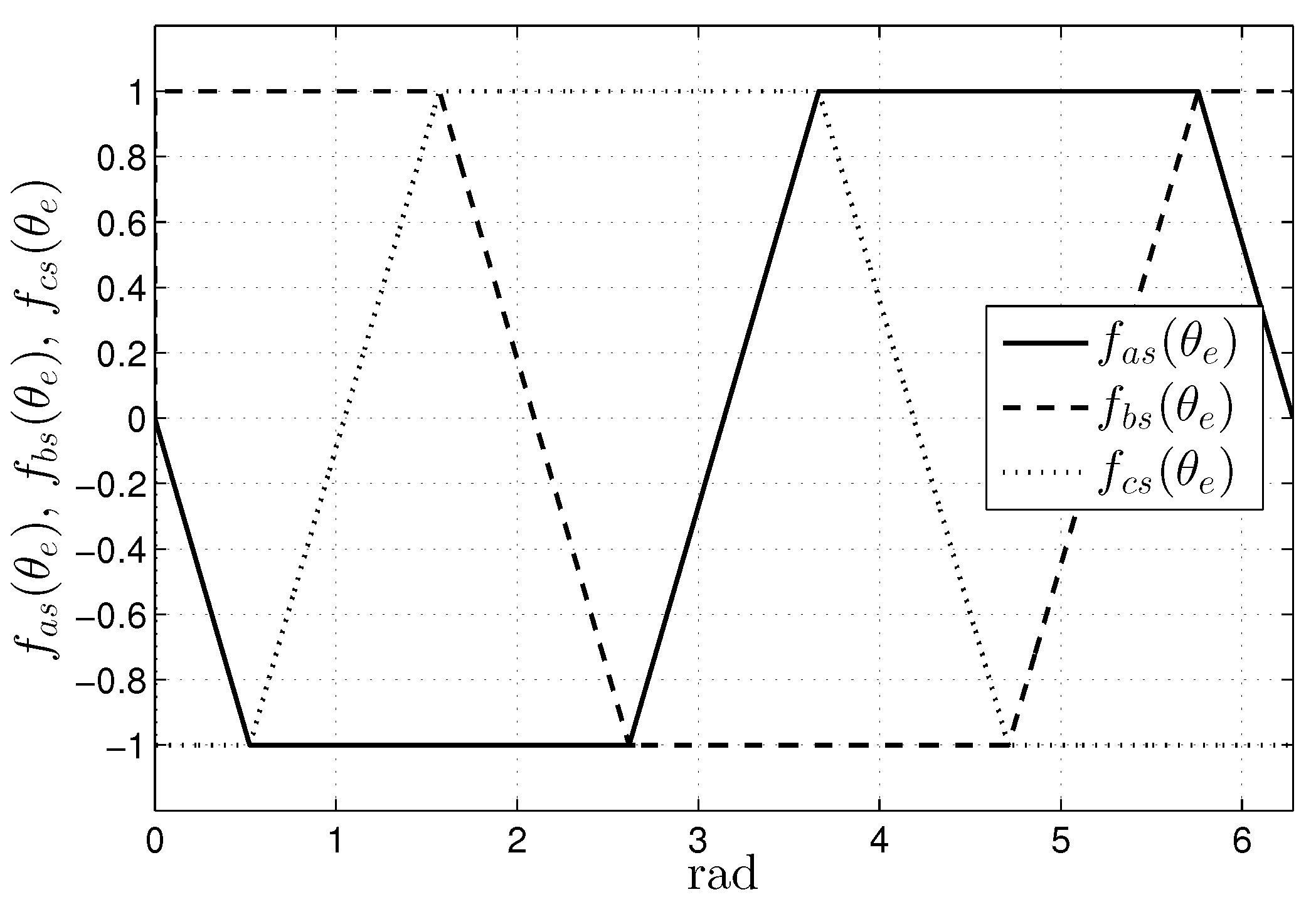
2.1. Mathematical Modeling of the BLDC Motor in Natural Variables

A mathematical model can be expressed in the following set of equations assuming a symmetrical three-phase BLDC motor while ignoring mutual inductance between phases and magnetic hysteresis [23]:

$$\begin{array}{ccc}\hfill \left[\begin{array}{c}{v}_{as}\\ v_{bs}\\ v_{cs}\end{array}\right]& =& \left[\begin{array}{ccc}{R}_s& 0& 0\\ 0& R_s& 0\\ 0& 0& R_s\end{array}\right]\left[\begin{array}{c}{i}_{as}\\ i_{bs}\\ i_{cs}\end{array}\right]+\left[\begin{array}{ccc}{L}_s& 0& 0\\ 0& L_s& 0\\ 0& 0& L_s\end{array}\right]\frac{d}{dt}\left[\begin{array}{c}{i}_{as}\\ i_{bs}\\ i_{cs}\end{array}\right]+\left[\begin{array}{c}{e}_{as}\\ e_{bs}\\ e_{cs}\end{array}\right]\hfill \end{array}$$

(1)

where $v_{as}$, $v_{bs}$, $v_{cs}$ and $i_{as}$, $i_{bs}$, $i_{cs}$ are the stator phase voltages and stator phase currents respectively, $R_s$ is the stator phase resistance and $L_s$ being the stator inductance. The induced stator back-EMF waveforms are denoted by $e_{as}$, $e_{bs}$ and $e_{cs}$ and can be written as:

$$\begin{array}{c}\hfill \left[\begin{array}{c}{e}_{as}\\ e_{bs}\\ e_{cs}\end{array}\right]={\omega }_e{\lambda }_p\left[\begin{array}{c}{f}_{as}\left({\theta }_e\right)\\ f_{bs}\left({\theta }_e\right)\\ f_{cs}\left({\theta }_e\right)\end{array}\right].\end{array}$$

(2)

where ${\omega }_e=d{\theta }_e/dt$ defines the electrical rotor velocity, ${\lambda }_p$ is the magnitud of the flux linkages generated by the permanent magnets, ${\theta }_e=\frac{p}{2}{\theta }_m$ represents electrical angular position of the rotor with p being the number of motor poles and ${\theta }_m$ representing the rotor mechanical position. The functions $f_{as}\left({\theta }_e\right)$, $f_{bs}\left({\theta }_e\right)$ and $f_{cs}\left({\theta }_e\right)$ are position dependent back-EMF waveform fundamental functions shown in Figure 1.

The following equation describes the electromagnetic torque generated by the motor:

$$T_e=[e_{as}{i}_{as}+e_{bs}{i}_{bs}+e_{cs}{i}_{cs}]\frac{1}{{\omega }_m}$$

(3)

and by substituting (2) in this equation, the electromagnetic torque can be expressed by:

$$T_e=\frac{p}{2}{\lambda }_p[f_{as}\left({\theta }_e\right)i_{as}+f_{bs}\left({\theta }_e\right)i_{bs}+f_{cs}\left({\theta }_e\right)i_{cs}].$$

(4)

To complete the mathematical model it is necessary to describe the equation of motion for the BLDC motor as:

$$J\frac{d{\omega }_m}{dt}+B{\omega }_m=(T_e-T_l).$$

(5)

From (1) and (5), the mathematical model results as:

$$\begin{array}{c}\hfill \begin{array}{cc}\hfill \frac{d{\omega }_m}{dt}& =\frac{T_e}{J}-\frac{T_l}{J}-\frac{B{\omega }_m}{J}\hfill \\ \hfill \frac{d{i}_{as}}{dt}& =-\frac{R_s}{L_s}{i}_{as}-\frac{p{\omega }_m{\lambda }_p}{2L_s}{f}_{as}\left({\theta }_e\right)+\frac{v_{as}}{L_s}\hfill \\ \hfill \frac{d{i}_{bs}}{dt}& =-\frac{R_s}{L_s}{i}_{bs}-\frac{p{\omega }_m{\lambda }_p}{2L_s}{f}_{bs}\left({\theta }_e\right)+\frac{v_{bs}}{L_s}\hfill \\ \hfill \frac{d{i}_{cs}}{dt}& =-\frac{R_s}{L_s}{i}_{cs}-\frac{p{\omega }_m{\lambda }_p}{2L_s}{f}_{cs}\left({\theta }_e\right)+\frac{v_{cs}}{L_s}.\hfill \end{array}\end{array}$$

(6)

2.2. Mathematical Model of the BLDC Motor in $(\alpha ,\beta )$ Reference Frame

A useful transformation known as $(\alpha ,\beta )$ transformation is commonly used to express a three phase system as an equivalent set of two variable equations system [24]. Three phase variables are transformed from a three phase reference frame to an orthogonal two-axis reference frame simplifying subsequent analysis. The following matrix is used to transform the BLDC model (6):

$$\begin{array}{c}\hfill T_{\alpha ,\beta }=\frac{2}{3}\left[\begin{array}{ccc}1& -\frac{1}{2}& -\frac{1}{2}\\ 0& \frac{\sqrt{3}}{2}& -\frac{\sqrt{3}}{2}\end{array}\right].\end{array}$$

(7)

The transformation matrix (7) is applied to (1) to obtain the voltage equations for the machine in $(\alpha ,\beta )$ reference frame described as:

$$\begin{array}{c}\hfill \begin{array}{cc}\hfill v_{\alpha }& =R_s{i}_{\alpha }+L_s\frac{d{i}_{\alpha }}{dt}+{\lambda }_p{\displaystyle \frac{p}{2}}{\omega }_m{f}_{\alpha }\left({\theta }_e\right)\hfill \\ \hfill v_{\beta }& =R_s{i}_{\beta }+L_s\frac{d{i}_{\beta }}{dt}+{\lambda }_p{\displaystyle \frac{p}{2}}{\omega }_m{f}_{\beta }\left({\theta }_e\right).\hfill \end{array}\end{array}$$

(8)

Furthermore, by applying this transformation to (4) the electromagnetic torque is given in $(\alpha ,\beta )$ reference frame as:

$$\begin{array}{c}\hfill T{e}_{\alpha ,\beta }=\frac{3p{\lambda }_p}{4}[f_{\alpha }\left({\theta }_e\right)i_{\alpha }+f_{\beta }\left({\theta }_e\right)i_{\beta }].\end{array}$$

(9)

Then, it is possible to describe the mathematical model for the BLDC motor in $(\alpha ,\beta )$ reference frame:

$$\begin{array}{c}\hfill \begin{array}{cc}\hfill \frac{d{\omega }_m}{dt}& =\frac{3p{\lambda }_p}{4J}[f_{\alpha }\left({\theta }_e\right)i_{\alpha }+f_{\beta }\left({\theta }_e\right)i_{\beta }]-\frac{T_l}{J}-\frac{B{\omega }_m}{J}\hfill \\ \hfill \frac{d{i}_{\alpha }}{dt}& =-\frac{R_s}{L_s}{i}_{\alpha }-\frac{p{\omega }_m{\lambda }_p}{2L_s}{f}_{\alpha }\left({\theta }_e\right)+\frac{u_{\alpha }}{L_s}\hfill \\ \hfill \frac{d{i}_{\beta }}{dt}& =-\frac{R_s}{L_s}{i}_{\beta }-\frac{p{\omega }_m{\lambda }_p}{2L_s}{f}_{\beta }\left({\theta }_e\right)+\frac{u_{\beta }}{L_s}.\hfill \end{array}\end{array}$$

(10)

2.3. Mathematical Model of the BLDC Motor in $(d,q)$ Reference Frame

Field orientation of three-phase motors is widely used since it permits to represent the dynamics of motors similarly to that of DC motors, which is characterized by constant variables. Park transformation, also known as $(d,q)$ transformation, is used to represent a stationary system in a rotary reference frame that is fixed to the magnetic fluxes generated in the motor [24]. BLDC motors commonly have hall effect sensors which are used for rotor position but only used as a six-position profile, it is then necessary to use an encoder or resolver to sense the electrical position of the rotor at all time instances. The transformation is achieved using an orthogonal transformation matrix expressed by:

$$\begin{array}{c}\hfill T_{d,q}=\left[\begin{array}{cc}cos\left({\theta }_e\right)& sin\left({\theta }_e\right)\\ -sin\left({\theta }_e\right)& cos\left({\theta }_e\right)\end{array}\right].\end{array}$$

(11)

Applying $(d,q)$ transformation to (8) and (9) gives the $(d,q)$ voltage equations:

$$\begin{array}{c}\hfill \begin{array}{cc}\hfill v_d& =R_s{i}_d+L_s\frac{d{i}_d}{dt}-{\omega }_e{L}_s{i}_q+{\lambda }_p{\displaystyle \frac{p}{2}}{\omega }_m{f}_d\left({\theta }_e\right)\hfill \\ \hfill v_q& =R_s{i}_q+L_s\frac{d{i}_q}{dt}+{\omega }_e{L}_s{i}_d+{\lambda }_p{\displaystyle \frac{p}{2}}{\omega }_m{f}_q\left({\theta }_e\right)\hfill \end{array}\end{array}$$

(12)

and the $(d,q)$ electromagnetic torque equation:

$$T{e}_{d,q}=\frac{3p{\lambda }_p}{4}[f_d\left({\theta }_e\right)i_d+f_q\left({\theta }_e\right)i_q].$$

(13)

From (12) and (13), the $(d,q)$ mathematical model of the BLDC motor can be written as:

$$\begin{array}{c}\hfill \begin{array}{cc}\hfill \frac{d{\omega }_m}{dt}& =\frac{3p{\lambda }_p}{4J}[f_d\left({\theta }_e\right)i_d+f_q\left({\theta }_e\right)i_q]-\frac{T_l}{J}-\frac{B{\omega }_m}{J}\hfill \\ \hfill \frac{d{i}_d}{dt}& =-\frac{R_s}{L_s}{i}_d+\frac{p}{2}{\omega }_m{i}_q-\frac{p{\omega }_m{\lambda }_p}{2L_s}{f}_d\left({\theta }_e\right)+\frac{u_d}{L_s}\hfill \\ \hfill \frac{d{i}_q}{dt}& =-\frac{R_s}{L_s}{i}_q-\frac{p}{2}{\omega }_m{i}_d-\frac{p{\omega }_m{\lambda }_p}{2L_s}{f}_q\left({\theta }_e\right)+\frac{u_q}{L_s}.\hfill \end{array}\end{array}$$

(14)

It is important to note that Park transformation is designed for motors with sinusoidal shaped back-EMF. The BLDC motor has non-sinusoidal back-EMF fundamental functions as shown in Figure 1; therefore, to achieve correct field orientation a modification to standard Park transformation is needed (see [7]). Figure 2 shows the back-EMF fundamental functions of the motor in $(d,q)$ reference frame.

Evidently, a modification to standard $(d,q)$ transformation is required to obtain the mathematical model of the BLDC motor with time-invariant variables.

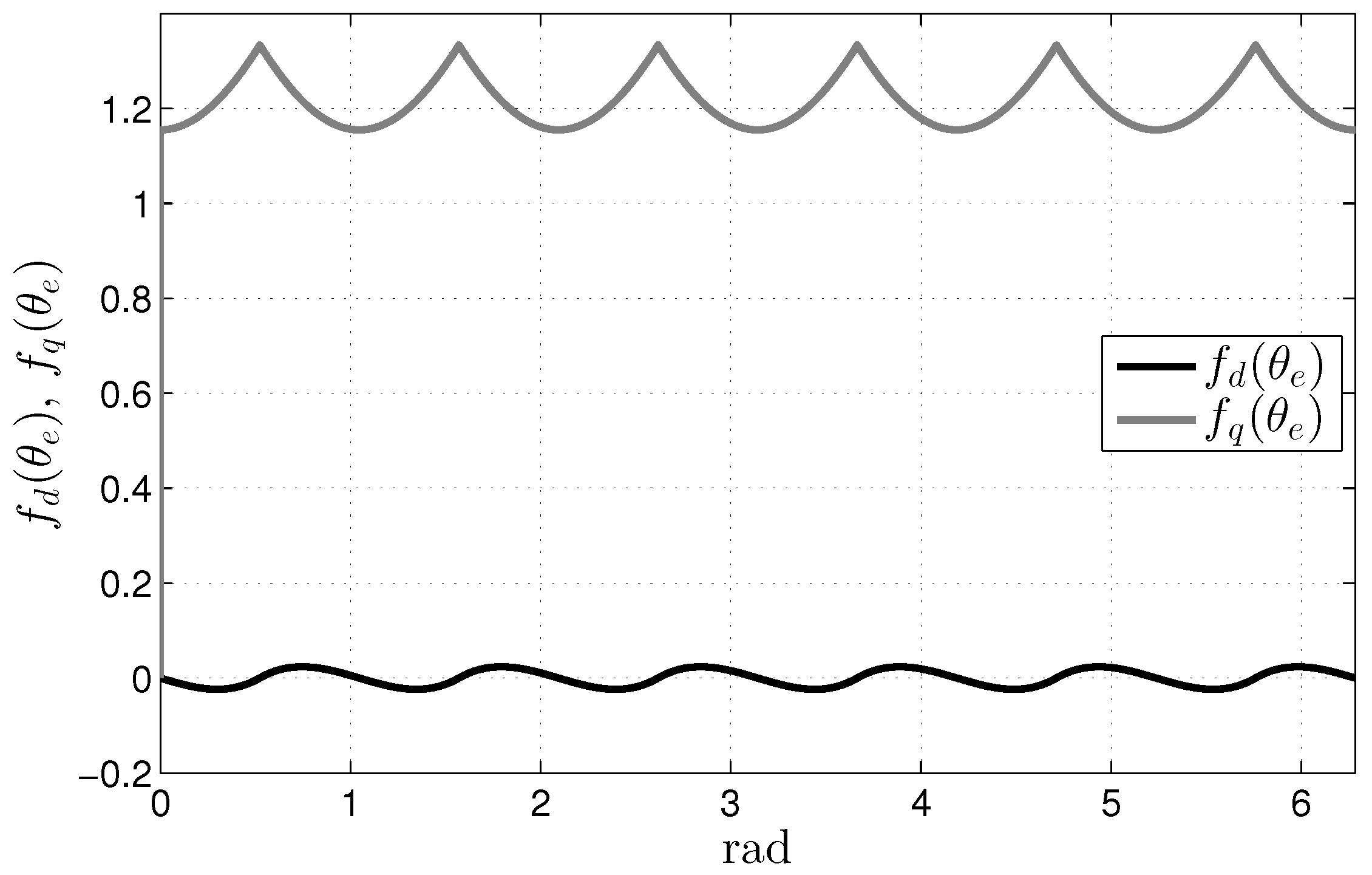
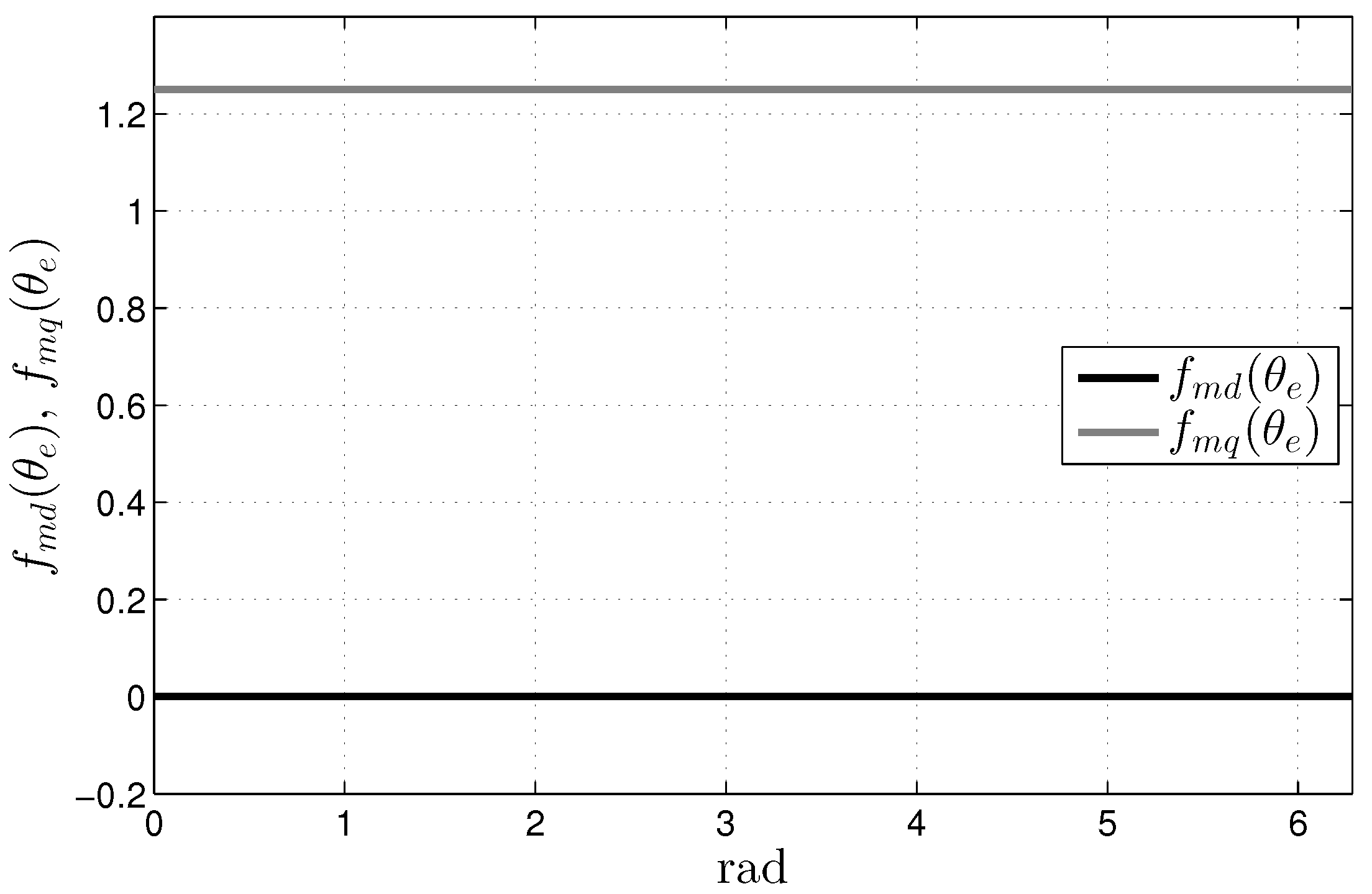
2.4. Mathematical Model of the BLDC Motor in Modified-$(d,q)$ Reference Frame

A modification to Park transformation is described in [7,8], where two new variables are presented to compensate amplitude and position error resulting from standard $(d,q)$ transformation. An offset to the rotor position, denoted as $\mu$, is introduced to fix the d component of the back-EMF fundamental function along the d axis of the reference frame. A variable $\kappa$ is used to compensate for the amplitude variations in the q-component of the back-EMF fundamental functions. The modified transformation matrix is defined as:

$$\begin{array}{c}\hfill M_{d,q}={\displaystyle \frac{1}{\kappa }}\left[\begin{array}{cc}cos({\theta }_e+\mu )& sin({\theta }_e+\mu )\\ -sin({\theta }_e+\mu )& cos({\theta }_e+\mu )\end{array}\right].\end{array}$$

(15)

where the compensation variables are described as:

$$\begin{array}{c}\hfill \begin{array}{cc}\hfill \kappa & =\frac{\sqrt{f_{\alpha }{\left({\theta }_e\right)}^2+f_{\beta }{\left({\theta }_e\right)}^2}}{{\lambda }_p}\hfill \\ \hfill \mu & =ta{n}^{-1}\left(\frac{-f_{\alpha }\left({\theta }_e\right)}{f_{\beta }\left({\theta }_e\right)}\right)-{\theta }_e.\hfill \end{array}\end{array}$$

(16)

It is evident that this modified transformation is a generalization of Park transformation for non-sinusoidal back-EMF motors where $\mu =0$ and $\kappa =1$ for a sinusoidal machine.

The resulting back-EMF fundamental functions after modified transformation, denoted $f_{md}\left({\theta }_e\right)$ and $f_{mq}\left({\theta }_e\right)$, are shown in Figure 3. From this figure it is clear that the modified transformation successfully transforms non-sinusoidal variables to constant dc quantities which shows proper field orientation, thus, allowing control schemes for the BLDC motor to be designed similarly as other PMSM that have sinusoidal shaped back-EMF.

It is then necessary to express a mathematical model for the BLDC motor in this newly defined reference frame. Applying (15) into (8) gives the voltage equations in the modified-$(d,q)$ reference frame:

$$\begin{array}{c}\hfill \begin{array}{cc}\hfill v_{md}& =R_s{i}_{md}+L_s{\displaystyle \frac{1}{\kappa }}{\displaystyle \frac{d\kappa }{dt}}{i}_{md}+{\displaystyle \frac{p}{2}}{\omega }_m{L}_s{i}_{mq}+L_s{\displaystyle \frac{d\mu }{dt}}{i}_{mq}+L_s\frac{d{i}_{md}}{dt}+{\lambda }_p{\displaystyle \frac{p}{2}}{\omega }_m{f}_{md}\left({\theta }_e\right)\hfill \\ \hfill v_{mq}& =R_s{i}_{mq}+L_s{\displaystyle \frac{1}{\kappa }}{\displaystyle \frac{d\kappa }{dt}}{i}_{mq}-{\displaystyle \frac{p}{2}}{\omega }_m{L}_s{i}_{md}-L_s{\displaystyle \frac{d\mu }{dt}}{i}_{md}+L_s\frac{d{i}_{mq}}{dt}+{\lambda }_p{\displaystyle \frac{p}{2}}{\omega }_m{f}_{mq}\left({\theta }_e\right)\hfill \end{array}\end{array}$$

(17)

where $f_{md}\left({\theta }_e\right)$ is fixed to the d-axis of the modified reference frame and is equal to zero and $f_{mq}\left({\theta }_e\right)=1/{\kappa }^2$. Also, the electromagnetic torque (9) results in:

$$T{e}_{md,mq}=\frac{3{\kappa }^{2}p{\lambda }_p}{4}[f_{md}\left({\theta }_e\right)i_{md}+f_{mq}\left({\theta }_e\right)i_{mq}].$$

(18)

in this new reference frame.

From (17) and (18) and by substituting $f_{md}\left({\theta }_e\right)=0$ and $f_{mq}\left({\theta }_e\right)=1/{\kappa }^2$, we obtain the mathematical model for the BLDC motor in the modified-$(d,q)$ reference frame:

$$\begin{array}{c}\hfill \begin{array}{cc}\hfill \frac{d{\omega }_m}{dt}& =\frac{3p{\lambda }_p}{4J}{i}_{mq}-\frac{T_l}{J}-\frac{B{\omega }_m}{J}\hfill \\ \hfill \frac{d{i}_{md}}{dt}& =-\frac{R_s{i}_{md}}{L_s}-{\displaystyle \frac{1}{\kappa }}{\displaystyle \frac{d\kappa }{dt}}{i}_{md}-{\displaystyle \frac{p}{2}}{\omega }_m{i}_{mq}-{\displaystyle \frac{d\mu }{dt}}{i}_{mq}+{\displaystyle \frac{u_{md}}{L_s}}\hfill \\ \hfill \frac{d{i}_{mq}}{dt}& =-\frac{R_s{i}_{mq}}{L_s}-{\displaystyle \frac{1}{\kappa }}{\displaystyle \frac{d\kappa }{dt}}{i}_{mq}+{\displaystyle \frac{p}{2}}{\omega }_m{i}_{md}+{\displaystyle \frac{d\mu }{dt}}{i}_{md}-\frac{p{\omega }_m{\lambda }_p}{2{\kappa }^2{L}_s}+{\displaystyle \frac{u_{mq}}{L_s}}.\hfill \end{array}\end{array}$$

(19)

It is important to note that the differential equation for the rotor velocity of (19) results in a simplification of the rotor velocity equation in (14) by the modified transformation. This simplification allows the controller to be designed in a similar fashion as a PMSM as in [25].

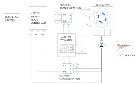
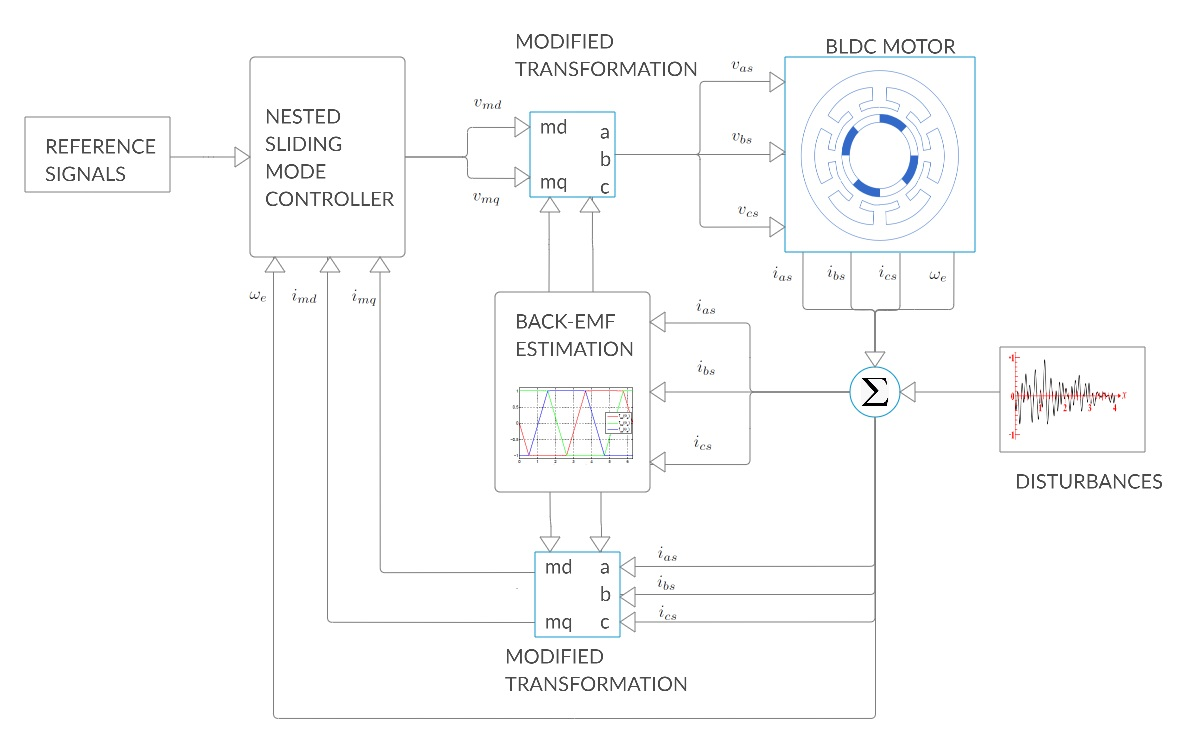
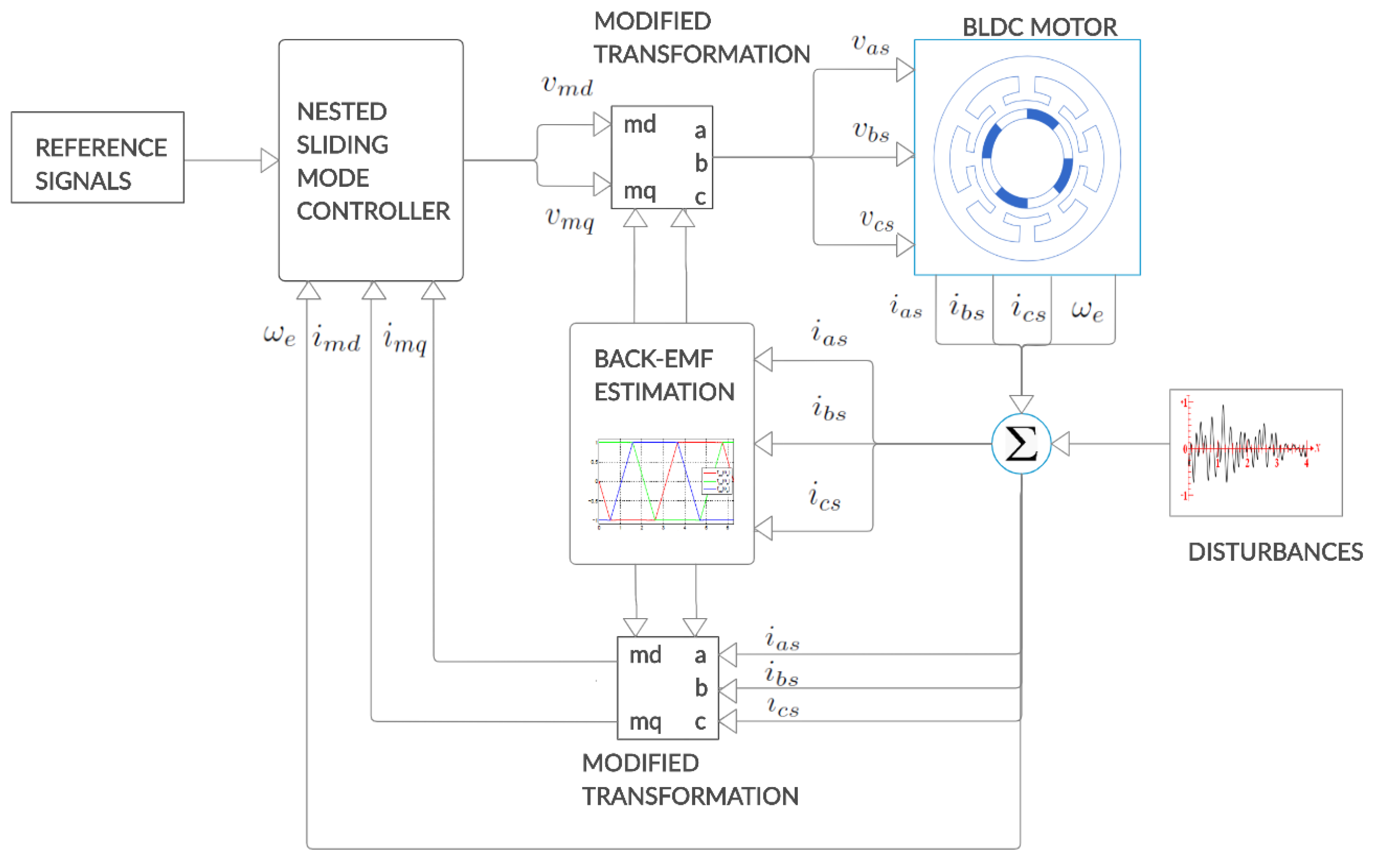
3. Back-EMF Observer and Controller Design

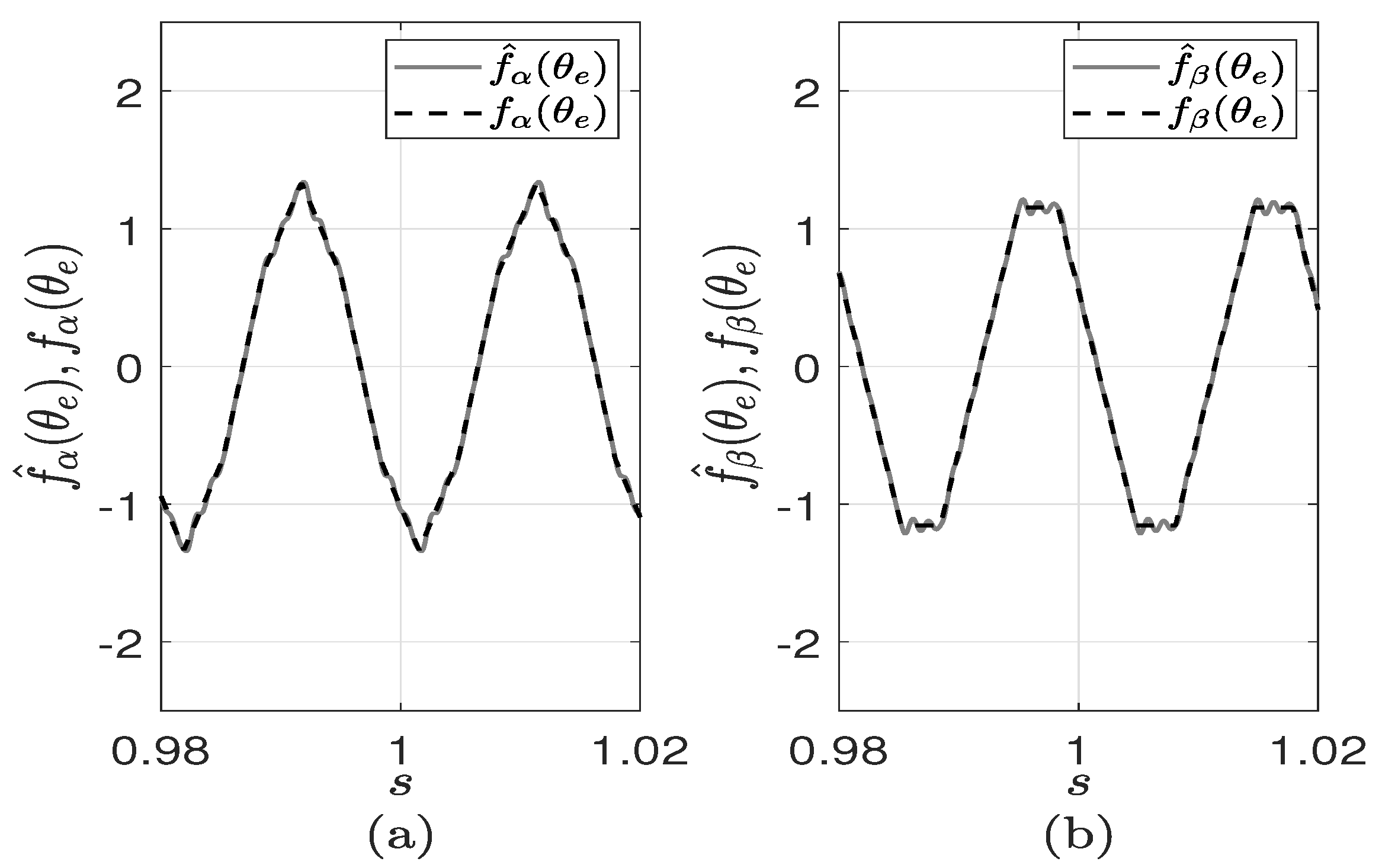
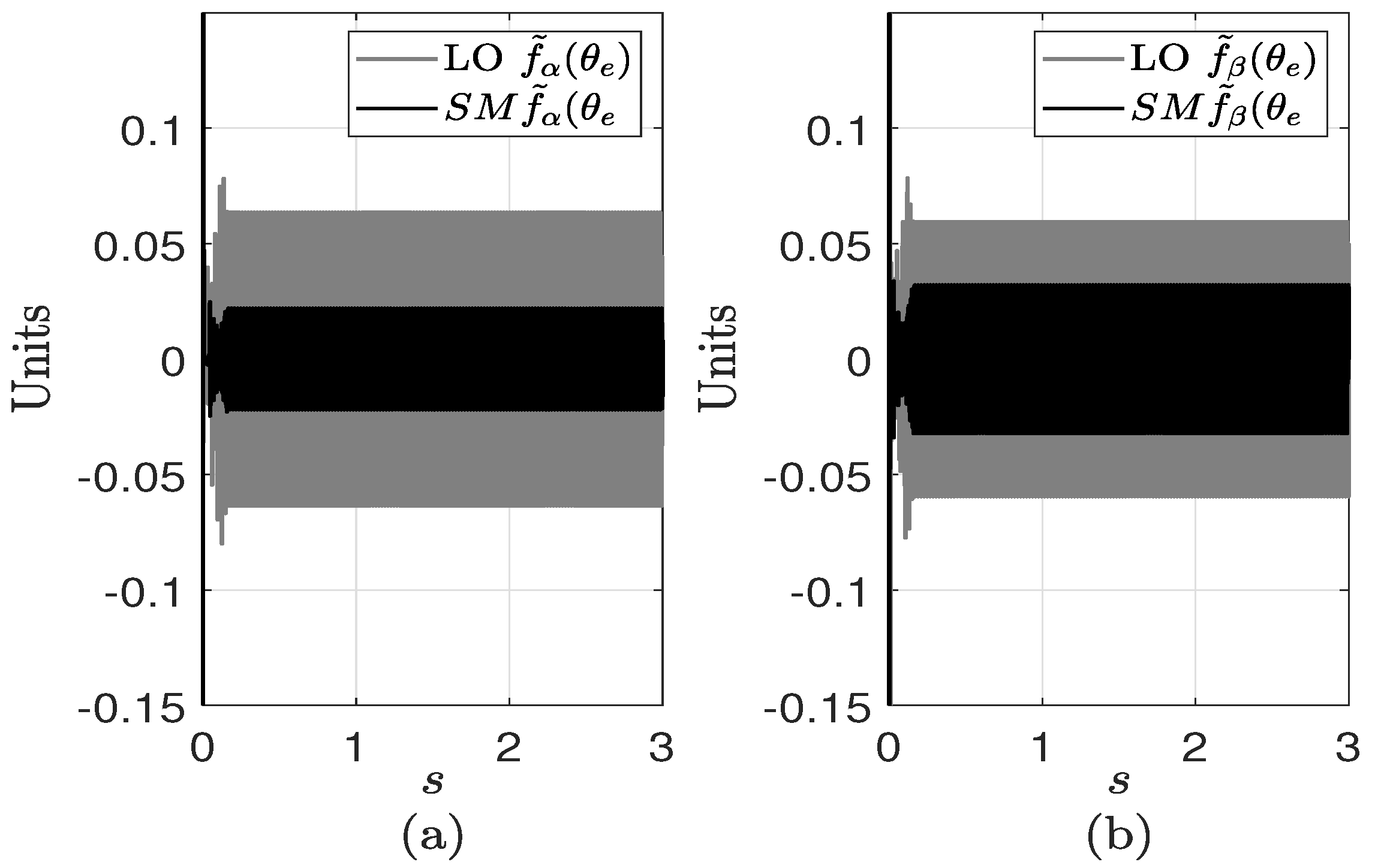
3.1. Sliding Mode Back-EMF Observer Design

The modified transformation described in (15) and (16) requires the back-EMF waveform fundamental functions to compensate the errors present in standard $(d,q)$ transformation. The back-EMF is not a measurable variable while the motor is being operated so an observer is used to estimate these variables while compensating simultaneously at all time instances the modified transformation. This information is needed Based on (10). As an addition to previous research [18], a sliding mode observer is proposed as:

$$\begin{array}{c}\hfill \begin{array}{cc}\hfill \frac{d{\widehat{i}}_{\alpha }}{dt}& =-\frac{R_s}{L_s}{\widehat{i}}_{\alpha }+\frac{u_{\alpha }}{L_s}+v_{\alpha }\hfill \\ \hfill \frac{d{\widehat{i}}_{\beta }}{dt}& =-\frac{R_s}{L_s}{\widehat{i}}_{\beta }+\frac{u_{\beta }}{L_s}+v_{\beta }.\hfill \end{array}\end{array}$$

(20)

Current estimation errors are then calculated as ${\tilde{i}}_{\alpha }=i_{\alpha }-{\widehat{i}}_{\alpha }$ and ${\tilde{i}}_{\beta }=i_{\beta }-{\widehat{i}}_{\beta }$ where ${\widehat{i}}_{\alpha }$ and ${\widehat{i}}_{\beta }$ are estimated currents. Deriving the estimation errors and using (20) and (10) the dynamics of the estimation errors result as:

$$\begin{array}{c}\hfill \begin{array}{cc}\hfill \frac{d{\tilde{i}}_{\alpha }}{dt}& =-\frac{R_s}{L_s}{\tilde{i}}_{\alpha }-\frac{p{\omega }_m{\lambda }_p}{2L_s}{f}_{\alpha }\left({\theta }_e\right)-v_{\alpha }\hfill \\ \hfill \frac{d{\tilde{i}}_{\beta }}{dt}& =-\frac{R_s}{L_s}{\tilde{i}}_{\beta }-\frac{p{\omega }_m{\lambda }_p}{2L_s}{f}_{\beta }\left({\theta }_e\right)-v_{\beta }.\hfill \end{array}\end{array}$$

(21)

Following a super-twisting sliding mode observer scheme, the observer injection signals are designed as:

$$\begin{array}{c}\hfill \begin{array}{cc}\hfill v_{\alpha }& =M_{\alpha }\sqrt{\left|{\tilde{i}}_{\alpha }\right|}sign\left({\tilde{i}}_{\alpha }\right)+n_0\hfill \\ \hfill {\dot{n}}_0& =-N_{\alpha }sign\left({\tilde{i}}_{\alpha }\right)\hfill \\ \hfill v_{\beta }& =M_{\beta }\sqrt{\left|{\tilde{i}}_{\alpha }\right|}sign\left({\tilde{i}}_{\alpha }\right)+n_1\hfill \\ \hfill {\dot{n}}_1& =-N_{\beta }sign\left({\tilde{i}}_{\alpha }\right)\hfill \end{array}\end{array}$$

(22)

where $M_{\alpha }$, $N_{\alpha }$, $M_{\beta }$ and $N_{\beta }$ are observer design gains set so that the current estimation errors tend asymptotically to zero as in [26], mathematical proof for the finite time convergence of the estimation errors can be found in [25]. The resulting closed loop sliding mode functions are:

$$\begin{array}{c}\hfill \begin{array}{cc}\hfill \frac{d{\tilde{i}}_{\alpha }}{dt}& =-M_{\alpha }\sqrt{\left|{\tilde{i}}_{\alpha }\right|}sign\left({\tilde{i}}_{\alpha }\right)+n_0-\frac{R_s}{L_s}{\tilde{i}}_{\alpha }-\frac{p{\omega }_m{\lambda }_p}{2L_s}{f}_{\alpha }\left({\theta }_e\right)\hfill \\ \hfill \frac{d{\tilde{i}}_{\beta }}{dt}& =-M_{\beta }\sqrt{\left|{\tilde{i}}_{\alpha }\right|}sign\left({\tilde{i}}_{\alpha }\right)+n_1-\frac{R_s}{L_s}{\tilde{i}}_{\beta }-\frac{p{\omega }_m{\lambda }_p}{2L_s}{f}_{\beta }\left({\theta }_e\right).\hfill \end{array}\end{array}$$

(23)

An important property of this observer is that the equivalent control signals from the observer defined from (22) tend to take the form of the unmeasurable terms of the system. When sliding mode occurs, the current estimation errors ${\tilde{i}}_{\alpha }$ and ${\tilde{i}}_{\beta }$ are equal to 0. From (21) one determines the following equivalent expressions for the injected signals:

$$\begin{array}{c}\hfill \begin{array}{c}\hfill v_{\alpha ,eq}=-\frac{p{\omega }_m{\lambda }_p}{2L_s}{f}_{\alpha }\left({\theta }_e\right)\\ \hfill v_{\beta ,eq}=-\frac{p{\omega }_m{\lambda }_p}{2L_s}{f}_{\beta }\left({\theta }_e\right)\end{array}\end{array}$$

(24)

and thus it is possible to estimate the back-EMF waveform fundamental functions needed in the compensation variables (16) used in the modified transformation as:

$$\begin{array}{c}\hfill \begin{array}{c}\hfill {\widehat{f}}_{\alpha }\left({\theta }_e\right)=-\frac{2L_s}{p{\omega }_m{\lambda }_p}{v}_{\alpha }\\ \hfill {\widehat{f}}_{\beta }\left({\theta }_e\right)=-\frac{2L_s}{p{\omega }_m{\lambda }_p}{v}_{\beta }.\end{array}\end{array}$$

(25)

Finally, a block scheme of the system is presented in Figure 4.

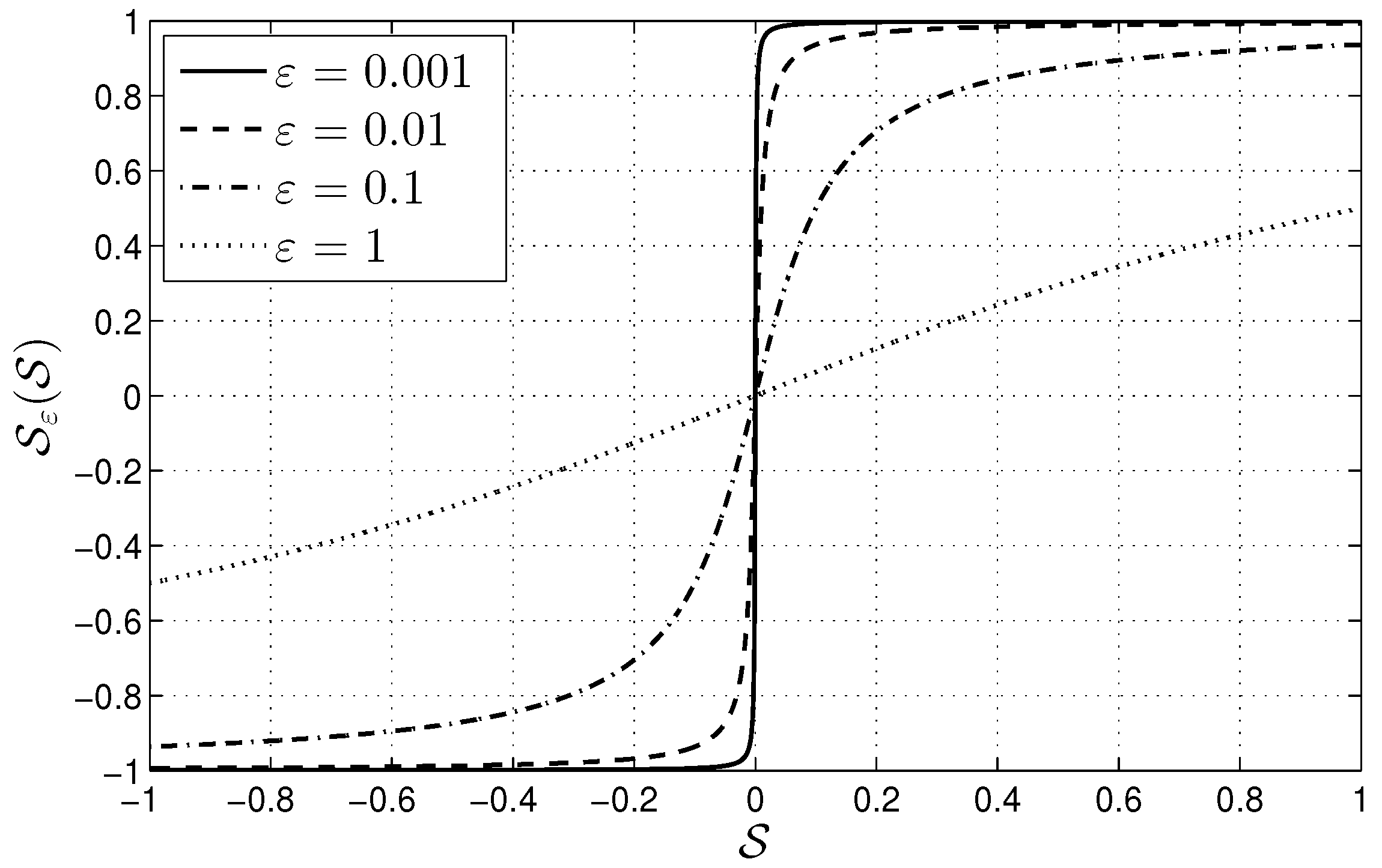
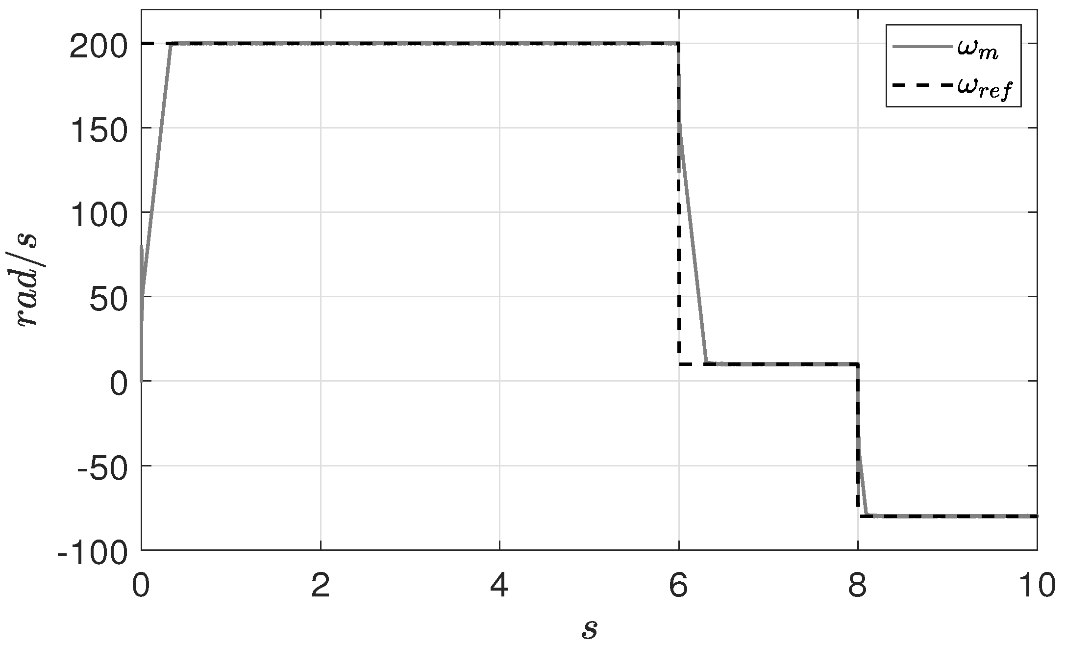
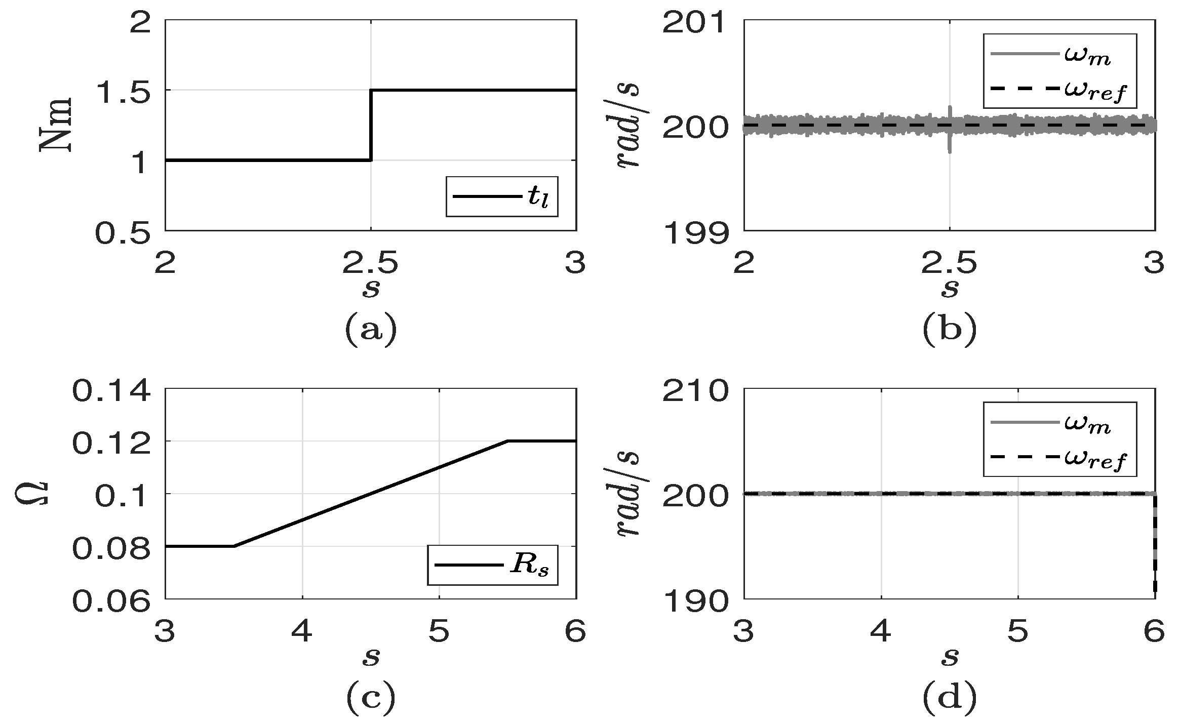
3.2. Nested High Order Sliding Mode Control Design

Following [18], speed control of the BLDC motor is designed by considering a mechanical angular velocity reference signal, ${\omega }_{ref}$, and determining the speed tracking error of the system as $z_1={\omega }_m-{\omega }_{ref}$ [27]. Deriving the tracking error and substituting from (19) the tracking error dynamic can be expressed as:

$$\begin{array}{c}\hfill {\dot{z}}_1=\frac{3p{\lambda }_p}{4J}{i}_{mq}-\frac{T_l}{J}-\frac{B{\omega }_m}{J}-{\dot{\omega }}_{ref}.\end{array}$$

(26)

The dynamic for the speed tracking error, $z_1$, is proposed as follows:

$$\begin{array}{c}\hfill {\dot{z}}_1=-k_1{\mathcal{S}}_{\epsilon }{z}_1\end{array}$$

(27)

where $k_1>0$. A sigmoid function ${\mathcal{S}}_{\epsilon }$ is used as an approximation of the sign function and is defined as:

$${\mathcal{S}}_{\epsilon }\left(S\right)=\frac{2}{\pi }arctan\frac{S}{\epsilon }.$$

(28)

A sigmoid function is used instead of a sign function because its derivative nature allows it to be implemented in the control design improving the response of the system to unmatched disturbances, see [17]. A sigmoid function is shown in Figure 5 for different values of $\epsilon$.

Clearly the approximation of the sign function is obtained for sufficiently small values of $\epsilon$.

Furthermore, from (26) and (27) a reference current is developed which acts as a pseudo-control law that incorporates the desired dynamics of the velocity tracking error as:

$$\begin{array}{c}\hfill i_{mqref}=\frac{4J}{3p{\lambda }_p}\left(-k_1{\mathcal{S}}_{\epsilon }\left(z_1\right)+\frac{B{\omega }_m}{J}+{\dot{\omega }}_{ref}\right).\end{array}$$

(29)

In field oriented control, the reference current $i_{mdref}$ is fixed to zero to maximize torque [24]. Current tracking variables are then defined as $z_{21}=i_{md}-i_{mdref}$ and $z_{22}=i_{mq}-i_{mqref}$ where:

$$\begin{array}{c}\hfill \begin{array}{cc}\hfill {\dot{z}}_{21}& =-\frac{R_s{i}_{md}}{L_s}-{\displaystyle \frac{1}{\kappa }}{\displaystyle \frac{d\kappa }{dt}}{i}_{md}-{\displaystyle \frac{p}{2}}{\omega }_m{i}_{mq}-{\displaystyle \frac{d\mu }{dt}}{i}_{mq}+{\displaystyle \frac{u_{md}}{L_s}}-\frac{d{i}_{mdref}}{dt}\hfill \\ \hfill {\dot{z}}_{22}& =-\frac{R_s{i}_{mq}}{L_s}-{\displaystyle \frac{1}{\kappa }}{\displaystyle \frac{d\kappa }{dt}}{i}_{mq}+{\displaystyle \frac{p}{2}}{\omega }_m{i}_{md}+{\displaystyle \frac{d\mu }{dt}}{i}_{md}-\frac{p{\omega }_m{\lambda }_p}{2{\kappa }^2{L}_s}+{\displaystyle \frac{u_{mq}}{L_s}}-\frac{d{i}_{mqref}}{dt}.\hfill \end{array}\end{array}$$

(30)

To force the current tracking errors to converge asymptotically to zero, a super-twisting second order sliding mode control law is proposed as:

$$\begin{array}{c}\hfill \begin{array}{cc}\hfill u_{md}& =-k_d{L}_s\sqrt{\left|z_{21}\right|}sign\left(z_{21}\right)+u_{d1}\hfill \\ \hfill {\dot{u}}_{d1}& =-k_{d1}sign\left(z_{21}\right)\hfill \\ \hfill u_{mq}& =-k_q{L}_s\sqrt{\left|z_{22}\right|}sign\left(z_{22}\right)+u_{q1}\hfill \\ \hfill {\dot{u}}_{q1}& =-k_{q1}sign\left(z_{22}\right)\hfill \end{array}\end{array}$$

(31)

with $k_d$, $k_{d1}$, $k_q$, $k_{q1}$ as positive control parameters designed so that $z_{21}$ y $z_{22}$ tend to zero in finite time. The closed-loop system is obtained by substituting control signals $u_{md}$ and $u_{mq}$ in (30) and by considering (26):

$$\begin{array}{c}\hfill \begin{array}{cc}\hfill \dot{z_1}& =\frac{3p{\lambda }_p}{4J}{z}_{22}-k_1{\mathcal{S}}_{\epsilon }\left(z_1\right)-\frac{T_l}{J}\hfill \\ \hfill {\dot{z}}_{21}& =-k_d\sqrt{\left|z_{21}\right|}sign\left(z_{21}\right)+u_{d1}+{\phi }_d\hfill \\ \hfill {\dot{u}}_{d1}& =-k_{d1}{L}_{s}sign\left(z_{21}\right)\hfill \\ \hfill {\dot{z}}_{22}& =-k_q\sqrt{\left|z_{22}\right|}sign\left(z_{22}\right)+u_{q1}+{\phi }_q\hfill \\ \hfill {\dot{u}}_{q1}& =-k_{q1}{L}_{s}sign\left(z_{22}\right)\hfill \end{array}\end{array}$$

(32)

with

$$\begin{array}{c}\hfill \begin{array}{cc}\hfill {\phi }_d& =-\frac{R_s{i}_{md}}{L_s}-{\displaystyle \frac{1}{\kappa }}{\displaystyle \frac{d\kappa }{dt}}{i}_{md}-{\displaystyle \frac{p}{2}}{\omega }_m{i}_{mq}-{\displaystyle \frac{d\mu }{dt}}{i}_{mq}-\frac{d{i}_{mdref}}{dt}\hfill \\ \hfill {\phi }_q& =-\frac{R_s{i}_{mq}}{L_s}-{\displaystyle \frac{1}{\kappa }}{\displaystyle \frac{d\kappa }{dt}}{i}_{mq}+{\displaystyle \frac{p}{2}}{\omega }_m{i}_{md}+{\displaystyle \frac{d\mu }{dt}}{i}_{md}-\frac{p{\omega }_m{\lambda }_p}{2{\kappa }^2{L}_s}-\frac{d{i}_{mqref}}{dt}.\hfill \end{array}\end{array}$$

(33)

Note that ${\phi }_d$ and ${\phi }_q$ are bounded functions, i.e., $|{\phi }_d|\le {\delta }_1>0$, and $|{\phi }_q|\le {\delta }_2>0$. This assumption is natural due to the limited energy supplied to the motor. Due to the boundness of such functions, control gains can be designed as in [27], mathematical proof of the convergence of current tracking errors in finite time is also shown in the previous reference.

When sliding mode occurs, $z_{21}=z_{22}=0$, the sliding mode dynamics reduce to the dynamics of the velocity tracking error as:

$${\dot{z}}_1=-k_1{\mathcal{S}}_{\epsilon }\left(z_1\right)-\frac{T_l}{J}.$$

(34)

where gain $k_1$ can be designed to guarantee that the speed tracking error tends asymptotically to zero in finite time [17].

Although the observer and the controller are separately designed, the separation principle is satisfied by achieving finite time convergence of the output tracking error of the system and ensuring that the current estimations errors tend asymptotically to zero, mathematical proof of the finite-time convergence is shown in [28].

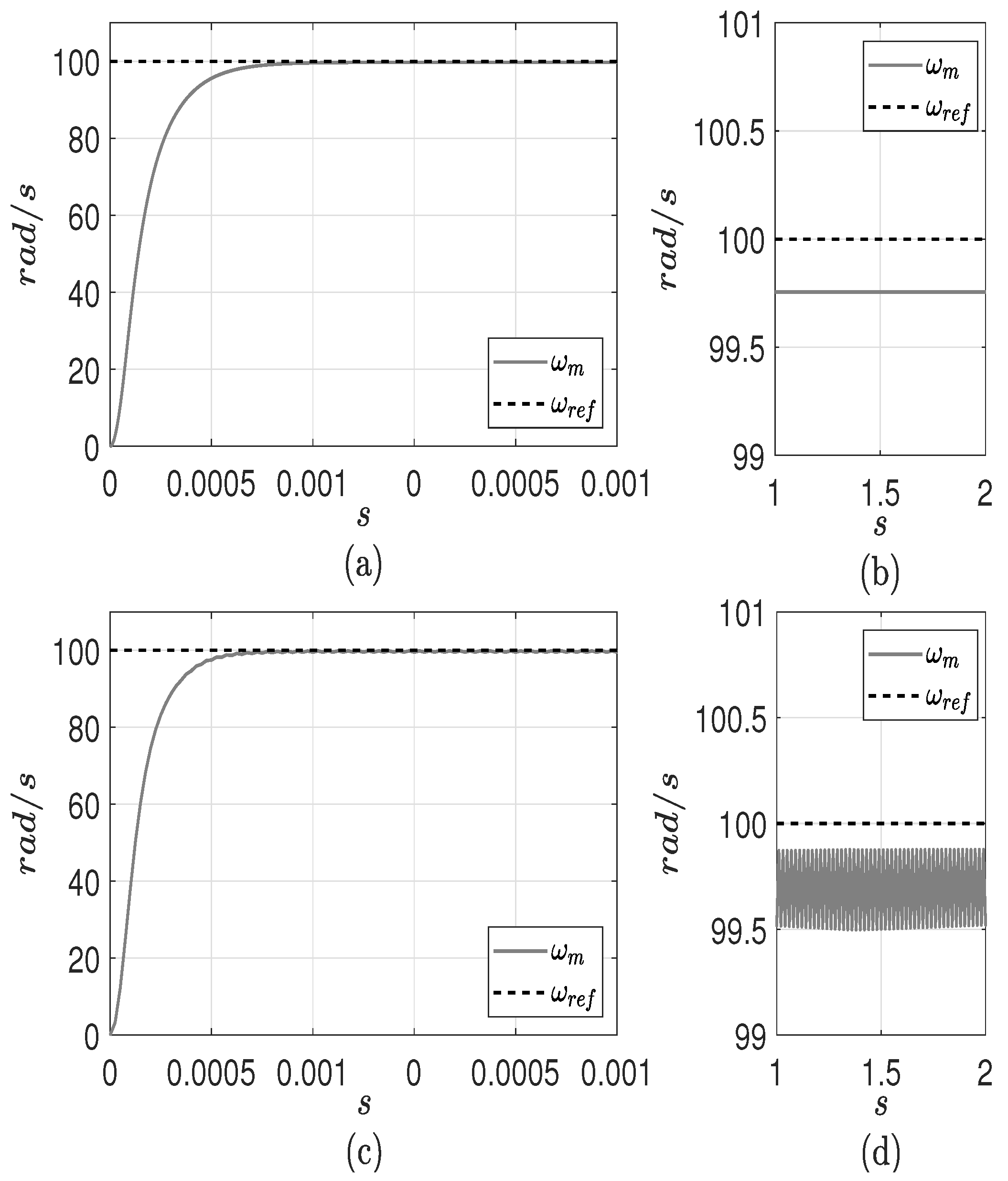
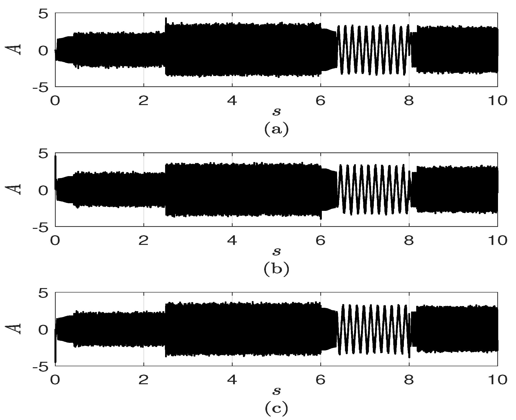
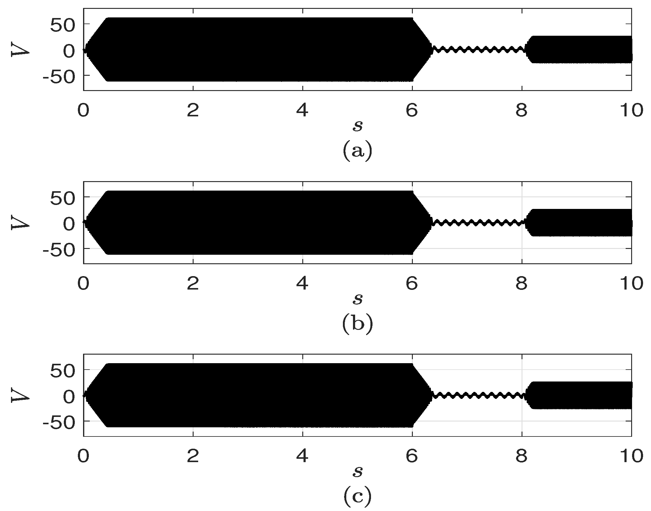
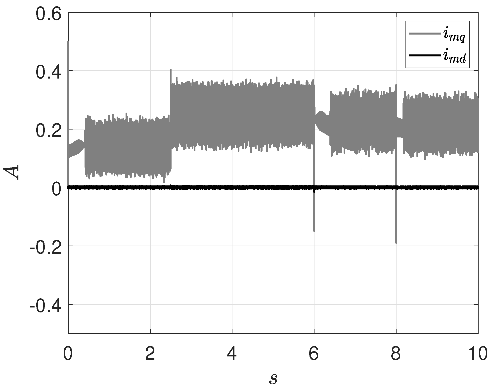
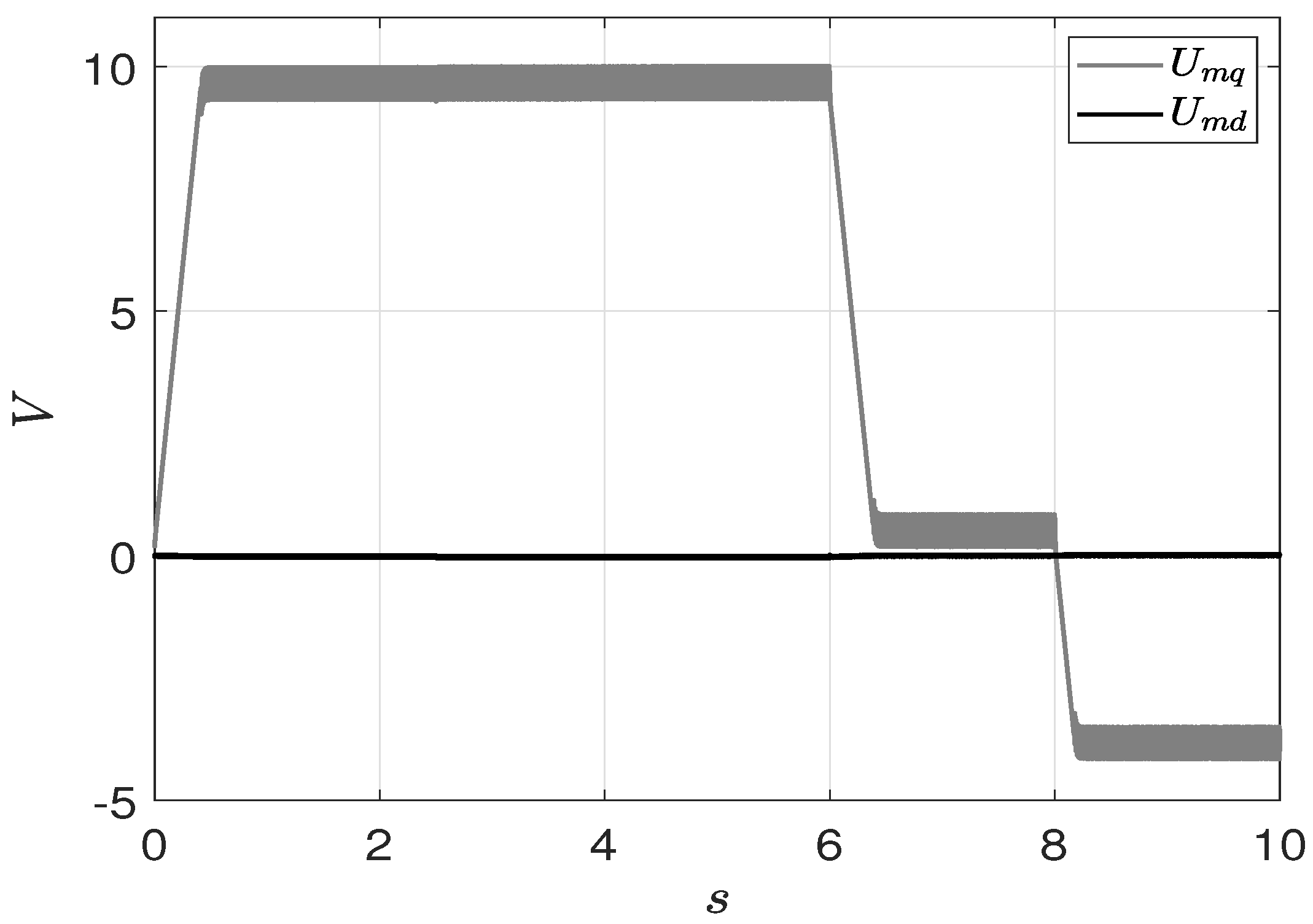
4. Simulation Results

Simulations are carried out to verify the performance of the designed observer and controller. To emulate real-time experimentation noise is introduced to the current and speed signals and delays in both input and output of the controller were applied along with load and coil resistance variations.

Table 1. BLDC Motor Parameters.

Parameter	Symbol	Value
Stator phase resistence	$R_s$	80 m$\Omega$
Stator phase inductance	$L_s$	0.15 mH
Number of poles	p	8
Nominal voltage	$V_{DC}$	48 V
Rotor inertia	J	0.00024 ${\mathrm{Kgm}}^2$
BEMF constant	${\lambda }_p$	0.1098 Vs/rad

details the parameters of the BLDC motor that was used.

It is possible to assume that BLDC motors have a sinusoidal shaped back-EMF as described in [2,3,4,5]. This assumption is done so by simplification or by mistake and can have a negative effect on system performance. In Figure 6, a comparison is done showing the performance of a sliding mode controller designed assuming a BLDC motor with sinusoidal shaped back-EMF when applied to both a sinusoidal and non-sinusoidal variable BLDC motor. Figure 6a shows the performance of a sliding mode controller designed assuming a BLDC motor with sinusoidal shaped back-EMF applied to a sinusoidal variable BLDC motor and Figure 6c displays the response of the same controller when paired to a non-sinusoidal variable machine, a close up on the performance of both cases is shown in Figure 6b and Figure 6d respectively.

Table 2. Precision error and chattering for sinusoidal and trapezoidal back-EMF assumption.

Back-EMF Type	Precision Error	Chattering
Sinusoidal	0.1%	0.2%
Trapezoidal	0.05%	≈0%

shows the precision error and chattering percentage of the performance of the system when assuming a sinusoidal and trapezoidal variable BLDC motor.

It is clear that both systems follow the reference signal as expected but the controller designed assuming a sinusoidal variable device exhibit oscillations around the reference signal. These variations result from the control law design when a sinusoidal variable motor is assumed and is applied to a more accurate mathematical model of the motor with non-sinusoidal back-EMF.

The modified transformation used in this paper requires information from the back-EMF fundamental functions which are not accessible during motor operation. There are several observer schemes used in back-EMF estimation that require heavy computation processing. A Luenberger observer is a common technique used in back-EMF estimation that is relatively uncomplicated and does not require heavy computational processing. In this paper, a super-twisting second-order sliding mode based observer is used due to its accurate estimation and simple design. Figure 7 and Figure 8 show the performance of the proposed observer and a Luenberger observer respectively. Figure 9 shows a comparison of both observers where it shows that the proposed observer has lower estimation errors when compared to a Luenberger observer.

For a proper analysis, a modified transformation has been used to obtain an accurate model of the motor and subsequent controller design. The design gains of the system are presented in

Table 3. Design Gains.

Parameter	Symbol	Value
Observer gain	$M_{\alpha }$	6000
Observer gain	$N_{\alpha }$	2000
Observer gain	$M_{\beta }$	6000
Observer gain	$N_{\beta }$	2000
Controller gain	$k1$	2000
Controller gain	$k_d$	2500
Controller gain	$k_{d1}$	35,000
Controller gain	$k_q$	2500
Controller gain	$k_{q1}$	35,000

which were defined by experimental tuning.

Furthermore, to test the response of the system for different rotor velocities, an angular velocity reference signal is specified as:

$$\begin{array}{c}\hfill {\omega }_{ref}=\left\{\begin{array}{cc}200\mathrm{rad}/\mathrm{s};& 0 \mathrm{s}\le t<5 \mathrm{s}\\ 10\mathrm{rad}/\mathrm{s};& 5 \mathrm{s}\le t<8 \mathrm{s}\\ -80\mathrm{rad}/\mathrm{s};& 8 \mathrm{s}\le t<10 \mathrm{s}.\end{array}\right.\end{array}$$

(35)

To analyze the robustness of the designed controller to unmatched disturbances, a variation to the load torque of the motor is used. Additionally, a gradual increase of 50% of the stator resistance is introduced to simulate the effect of temperature rise in the motor coils. These variations have the following form:

$$\begin{array}{c}\hfill t_l=\left\{\begin{array}{cc}1\mathrm{Nm};& t\le 2.5 \mathrm{s}\\ 1.5\mathrm{Nm};& t>2.5s\end{array}\right.\end{array}$$

(36)

and

$$\begin{array}{c}\hfill R_s=\left\{\begin{array}{cc}0.08\Omega ;& t\le 3.5 \mathrm{s}\\ 0.02t+0.01\Omega ;& 3.5 \mathrm{s}\le t\le 5.5 \mathrm{s}\\ 0.12\Omega ;& t>5.5s.\end{array}\right.\end{array}$$

(37)

Besides, 5% noise is introduced to the current and speed signals simulating real-time readings from sensors as well as signal delays in both sensors and control signals. The output of the system is shown in Figure 10. It is easy to see that the motor is able to follow the desired reference signal at positive and negative velocities with zero crossing and it also shows good performance at low speed where traditional observer-based controllers usually tend to show performance degradation.

The introduced variations are shown in Figure 11a,c and the figures Figure 11b,d display a zoom of the output of the system at the time instances where these perturbations are introduced. From these figures it is clear that the designed controller is able to reject unmatched disturbances such as load torque variations and shows robustness to parametric variations. The currents in natural variables $i_a$, $i_b$ and $i_c$ are shown in Figure 12 and the control signals in natural variables $u_a$, $u_b$ and $u_c$ are described in Figure 13. Also, the currents and control voltages in modified-$(d,q)$ are shown in Figure 14 and Figure 15 respectively. These figures show the response of the control voltages and the sensed currents under the presence of the simulated noise and delay. Furthermore, the current Figure 12 and Figure 14 show the effect of the introduced load variation at 2.5 s.

The modified-$(d,q)$ transformation described in this paper requires the estimation of the back-EMF fundamental functions to compensate for the error resulting from standard $(d,q)$ transformation. Figure 16a and Figure 17a show the correct estimated back-EMF fundamental functions ${\widehat{f}}_{\alpha }\left({\theta }_e\right)$ and ${\widehat{f}}_{\beta }\left({\theta }_e\right)$. The transient responses of both estimations are shown in Figure 16b and Figure 17b. The estimation of these functions uses information from the measurable variables that are simulated with noise and signal delays. Figure 16c and Figure 17c show a zoom of the back-EMF estimation errors before parametric and load variations and a zoom of the estimation errors after the variations are presented is shown in Figure 16d and Figure 17d. From these figures, it is clear that the observer is able to perform successfully under these disturbances. The performance of the observer is further displayed in Figure 18a,b where it is shown that the estimation errors for the back-EMF functions are lower than 0.25 units for positive and negative speeds. Traditional observer-based controlled systems usually present degradation of performance at low speeds, such performance is also shown in the previous figures with estimation errors lower than 0.8 units.

Another characteristic that is important to note is the smooth torque as a result of the modified-$d,q$ transformation which is not an easy task with traditional controllers. Figure 19a shows the electromagnetic torque of the machine under ideal operation where smooth torque is reached during the steady state condition of the motor shown in Figure 19b as a result of the modified-$(d,q)$ transformation.

5. Discussion

Sliding mode controllers can be designed assuming a BLDC motor with sinusoidal back-EMF which simplifies the control law development but it has been shown to neglect accurate system behavior. To address this issue a modification of Park transformation has been implemented that allows proper motor modeling and controller design. An observer has been introduced to estimate the back-EMF functions needed for the modified-$(d,q)$ transformation. From the described modified transformation a nested high order sliding mode controller for speed control of a BLDC motor has been designed and simulated. The robustness of the system has been analyzed by introducing unmatched disturbances in the form of load torque variations and stator resistance parametric variations with sensor noise and signal delays to emulate real-time experimentation. The system showed a satisfactory response under the previously mentioned stressed conditions. Smooth torque is exhibited in the performance of the system as a result of ripple reduction by the modification introduced in the used transformation. Discrete-time modeling analysis and controller designed are foreseen as future work along with real-time experimentation of both continuous and discrete-time schemes and future implementation on mobile robotic systems and/or electric vehicles.

References

1. Hughes, A.; Drury, B. Electric Motors and Drives Fundamentals, Types and Applications; Elsevier/Newnes: Waltham, MA, USA, 2013. [Google Scholar]
2. Krause, P.; Wasynczuk, O.; Sudhoff, S.; Pekarek, S. Electric Motors and Drives Fundamentals, Types and Applications; Wiley-IEEE Press: Hoboken, NJ, USA, 2013. [Google Scholar]
3. Quintero-Manríquez, E.; Félix, R.A. Second-order sliding mode speed controller with anti-windup for BLDC motors. In Proceedings of the 2014 World Automation Congress (WAC), Waikoloa, HI, USA, 3–7 August 2014; pp. 610–615. [Google Scholar]
4. Gujjar, M.N.; Kumar, P. Comparative analysis of field oriented control of BLDC motor using SPWM and SVPWM techniques. In Proceedings of the 2017 2nd IEEE International Conference on Recent Trends in Electronics, Information Communication Technology (RTEICT), Bangalore, India, 19–20 May 2017; pp. 924–929. [Google Scholar]
5. Sharma, P.K.; Sindekar, A.S. Performance analysis and comparison of BLDC motor drive using PI and FOC. In Proceedings of the 2016 International Conference on Global Trends in Signal Processing, Information Computing and Communication (ICGTSPICC), Jalgaon, India, 22–24 December 2016; pp. 485–492. [Google Scholar]
6. Yousef, A.Y.; Abdelmaksoud, S.M. Review on Field Oriented Control of Induction Motor. Int. J. Res. Emerg. Sci. Technol. (IJREST) 2015, 2, 5–16. [Google Scholar]
7. Kshirsagar, P.; Krishnan, R. Efficiency improvement evaluation of non-sinusoidal back-EMF PMSM machines using field oriented current harmonic injection strategy. In Proceedings of the 2010 IEEE Energy Conversion Congress and Exposition, Atlanta, GA, USA, 12–16 September 2010; pp. 471–478. [Google Scholar]
8. Lazor, M.; Štulrajter, M. Modified field oriented control for smooth torque operation of a BLDC motor. In Proceedings of the 2016 Journal of Electrical Systems and Information Technology, Rajecke Teplice, Slovakia, 19–20 May 2014; pp. 180–185. [Google Scholar]
9. Devendra, P.; Alice, M.K.; Saibabu, C. Design and implementation methodology for rapid control prototyping of closed loop speed control for BLDC motor. J. Electr. Syst. Inf. Technol. 2018, 5, 99–111. [Google Scholar]
10. Suganthi, P.; Nagapavithra, S.; Umamaheswari, S. Modeling and simulation of closed loop speed control for BLDC motor. In Proceedings of the 2017 Conference on Emerging Devices and Smart Systems (ICEDSS), Tiruchengode, India, 3–4 March 2017; pp. 229–233.
11. Wang, H.; Li, P.; Shu, Y.; Kang, D. Double closed loop control for BLDC based on whole fuzzy controllers. In Proceedings of the 2017 2nd IEEE International Conference on Computational Intelligence and Applications (ICCIA), Beijing, China, 8–11 September 2017; pp. 487–491. [Google Scholar]
12. Walekar, V.R.; Murkute, S.V. Speed Control of BLDC Motor using PI and Fuzzy Approach: A Comparative Study. In Proceedings of the 2018 International Conference on Information, Communication, Engineering and Technology (ICICET), Pune, India, 29–31 August 2018; pp. 1–4. [Google Scholar]
13. Shao, Y.; Yang, R.; Guo, J.; Fu, Y. Sliding mode speed control for brushless DC motor based on sliding mode torque observer. In Proceedings of the 2015 IEEE International Conference on Information and Automation, Lijiang, China, 8–10 August 2015; pp. 2466–2470. [Google Scholar]
14. Delpoux, R.; Lin-Shi, X.; Brun, X. Torque ripple reductions for non-sinusoidal BEMF Motor: An observation based control approach. IFAC-PapersOnLine 2017, 50, 15766–15772. [Google Scholar] [CrossRef]
15. Levant, A. Sliding order and sliding accuracy in sliding mode control. Int. J. Control 1993, 58, 180–185. [Google Scholar] [CrossRef]
16. Utkin, V. Variable structure systems with sliding modes. IEEE Trans. Autom. Control 1977, 22, 212–222. [Google Scholar] [CrossRef]
17. Castillo, B.; di Gennaro, S.; Loukianov, A.; Rivera, J. Robust Nested Sliding Mode Regulation with Application to Induction Motors. In Proceedings of the 2007 American Control Conference, New York, NY, USA, 9–13 July 2007; pp. 5242–5247. [Google Scholar]
18. Munoz-Gomez, G.; Alanis, A.Y.; Rivera, J. Nested High Order Sliding Mode Controller Applied to a Brushless Direct Current Motor. IFAC-PapersOnLine 2018, 51, 174–179. [Google Scholar] [CrossRef]
19. Shao, Y.; Wang, B.; Yu, Y.; Dong, Q.; Tian, M.; Xu, D. An Integral Sliding Mode Back-EMF Observer for Position-Sensorless Permanent Magnet Synchronous Motor Drives. In Proceedings of the 2019 22nd International Conference on Electrical Machines and Systems (ICEMS), Harbin, China, 11–14 August 2019; pp. 1–5. [Google Scholar]
20. Liu, D.; Zhang, Y.; Pan, L. Back-EMF Estimation Based on Extended Kalman Filtering in Application of BLCD Motor. In Electrical, Information Engineering and Mechatronics; Wang, X., Wang, F., Zhong, S., Eds.; Lecture Notes in Electrical Engineering; Springer: London, UK, 2011; Volume 138, pp. 1955–1967. [Google Scholar]
21. Wang, T. An EMF Observer for PMSM Sensorless Drives Adaptive to Stator Resistance and Rotor Flux Linkage. IEEE J. Emerg. Sel. Top. Power Electron. 2019, 7, 1899–1913. [Google Scholar] [CrossRef]
22. Khorrami, F.; Krishnamurthy, P.; Melkote, H. Modeling and Adaptive Nonlinear Control of Electric Motors; Springer: Berlin/Heidelberg, Germany, 2003. [Google Scholar]
23. Krishnan, R. Permanent Magnet Synchronous and Brushless DC Motor Drives; CRC Pres: Boca Raton, FL, USA, 2010. [Google Scholar]
24. Utkin, V.I.; Guldner, J.; Shi, J. Sliding Mode Control in Electromechanical Systems; Taylor & Francis Ltd.: Philadelphia, PA, USA, 1999. [Google Scholar]
25. Di Gennaro, S.; Rivera, J.; Castillo-Toledo, B. Super-twisting sensorless control of permanent magnet synchronous motors. In Proceedings of the 49th IEEE Conference on Decision and Control (CDC), Atlanta, GA, USA, 15–17 December 2010; pp. 4018–4023. [Google Scholar]
26. Moreno, J.A.; Osorio, M. A Lyapunov approach to second-order sliding mode controllers and observers. In Proceedings of the 2008 47th IEEE Conference on Decision and Control, Cancun, Mexico, 9–11 December 2008; pp. 2856–2861. [Google Scholar]
27. Di Gennaro, S.; Domínguez, J.R.; Meza, M.A. Sensorless High Order Sliding Mode Control of Induction Motors With Core Loss. IEEE Trans. Ind. Electron. 2014, 61, 2678–2689. [Google Scholar] [CrossRef]
28. Domínguez, J.R.; Navarrete, A.; Meza, M.A.; Loukianov, A.G.; Cañedo, J. Digital Sliding-Mode Sensorless Control for Surface-Mounted PMSM. IEEE Trans. Ind. Inform. 2014, 10, 137–151. [Google Scholar] [CrossRef]
Figure 1. Back-EMF waveform fundamental functions f a s ( θ e ) , f b s ( θ e ) and f c s ( θ e ) .
Electronics 09 01041 g001
Figure 2. Back-EMF fundamental functions f d ( θ e ) and f q ( θ e ) in ( d , q ) reference frame.
Electronics 09 01041 g002
Figure 3. Back-EMF fundamental functions f m d ( θ e ) and f m q ( θ e ) in modified- ( d , q ) reference frame.
Electronics 09 01041 g003
Figure 4. Block Diagram of the developed system.
Electronics 09 01041 g004
Figure 5. Sigmoid function S ε for various ε values.
Electronics 09 01041 g005
Figure 6. ω r e f (dashed line), ω m (gray line) (a) Performance of the controller motor applied to a sinusoidal BLDC motor. (c) Performance of the controller applied to a non-sinusoidal BLDC motor. (b,d) Zoom of the figures on the left.
Electronics 09 01041 g006
Figure 7. (a) Sliding mode based observer back-EMF function f α estimation; (b) Sliding mode based observer back-EMF function f β estimation.
Electronics 09 01041 g007
Figure 8. (a) Luenberger observer back-EMF function f α estimation; (b) Luenberger observer back-EMF function f β estimation.
Electronics 09 01041 g008
Figure 9. (a) Comparison of Luenberger and sliding mode based observer f α estimation error; (b) Comparison of Luenberger and sliding mode based observer f β estimation error.
Electronics 09 01041 g009
Figure 10. Rotor angular velocity reference signal ω r e f and motor angular velocity ω m .
Electronics 09 01041 g010
Figure 11. (a) Load torque t l variation; (b) Zoom of ω r e f , ω m at 2   s t < 3   s ; (c) Stator resistance R s variation; (d) Zoom of ω r e f , ω m at 3   s t < 6   s .
Electronics 09 01041 g011
Figure 12. (a) Stator currents i a ; (b) Stator current i b ; (c) Stator Current i c .
Electronics 09 01041 g012
Figure 13. (a) Control voltage u a ; (b) Control voltage u b ; (c) Control voltage u c .
Electronics 09 01041 g013
Figure 14. Stator currents in modified- ( d , q ) .
Electronics 09 01041 g014
Figure 15. Control voltage in modified- ( d , q ) .
Electronics 09 01041 g015
Figure 16. (a) Estimated back-EMF fundamental function f ^ α ( θ e ) . (b) Transient response close up of the estimation of the observer. (c) Zoom of f ^ α ( θ e ) estimation at 0.5   s t < 1   s . (d) Zoom of f ^ α ( θ e ) estimation at 5.5   s t < 6   s .
Electronics 09 01041 g016
Figure 17. (a) Estimated back-EMF fundamental function f ^ β ( θ e ) . (b) Transient response close up of the estimation of the observer. (c) Zoom of f ^ β ( θ e ) estimation at 0.5   s t < 1   s . (d) Zoom of f ^ β ( θ e ) estimation at 5.5   s t < 6   s .
Electronics 09 01041 g017
Figure 18. (a) Estimation error f ˜ α ( θ e ) . (b) Estimation error f ˜ β ( θ e ) .
Electronics 09 01041 g018
Figure 19. (a) Electromagnetic torque t e . (b) Electromagnetic torque during steady state condition.
Electronics 09 01041 g019