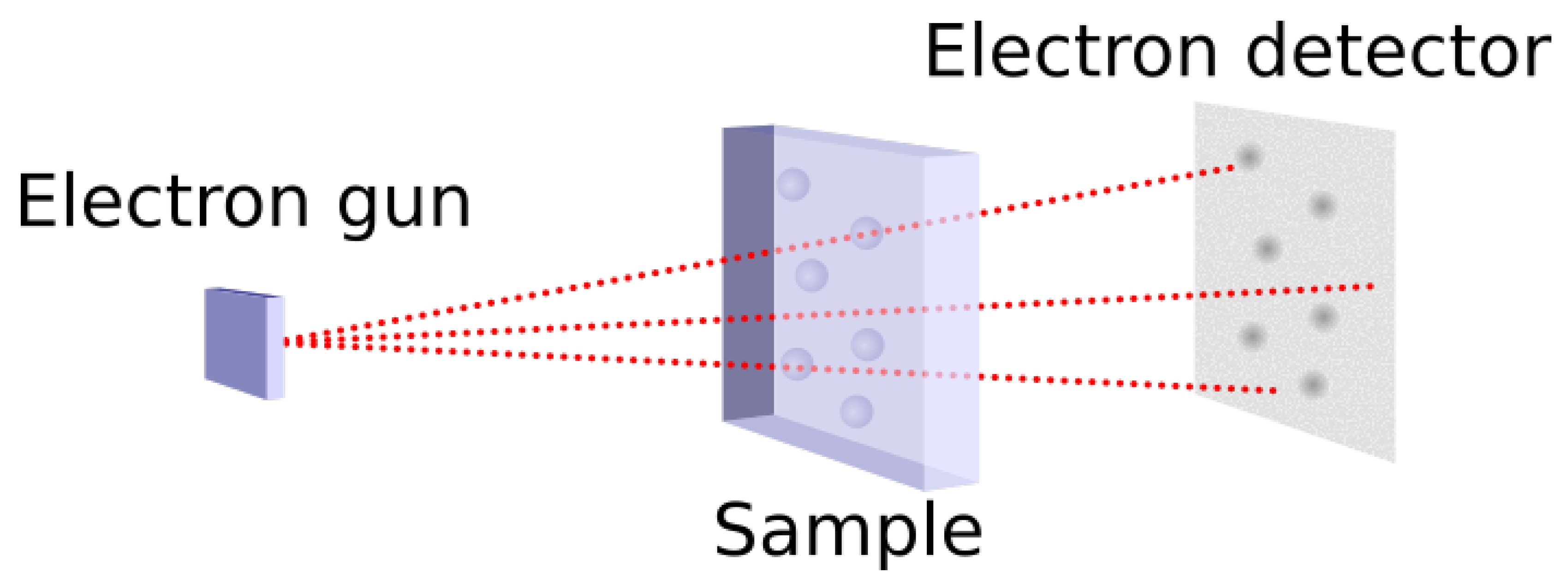
Figure 1.
Principle of the TEM.
Figure 1.
Principle of the TEM.
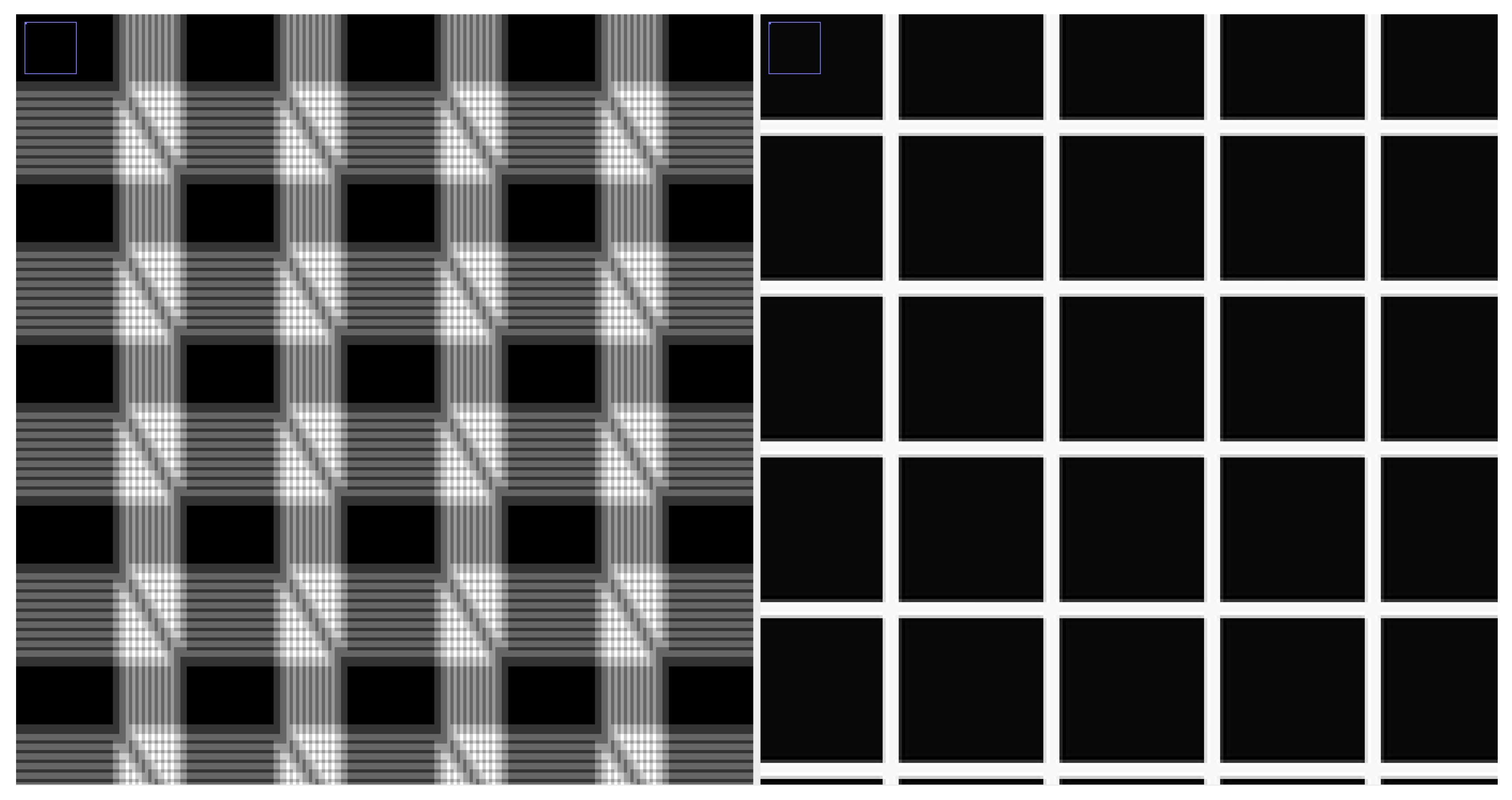
Figure 2.
Phantom movie (grid, detail), an average of 10 frames, nth frame shifted by the vector , before global alignment (left), after global alignment (right).
Figure 2.
Phantom movie (grid, detail), an average of 10 frames, nth frame shifted by the vector , before global alignment (left), after global alignment (right).
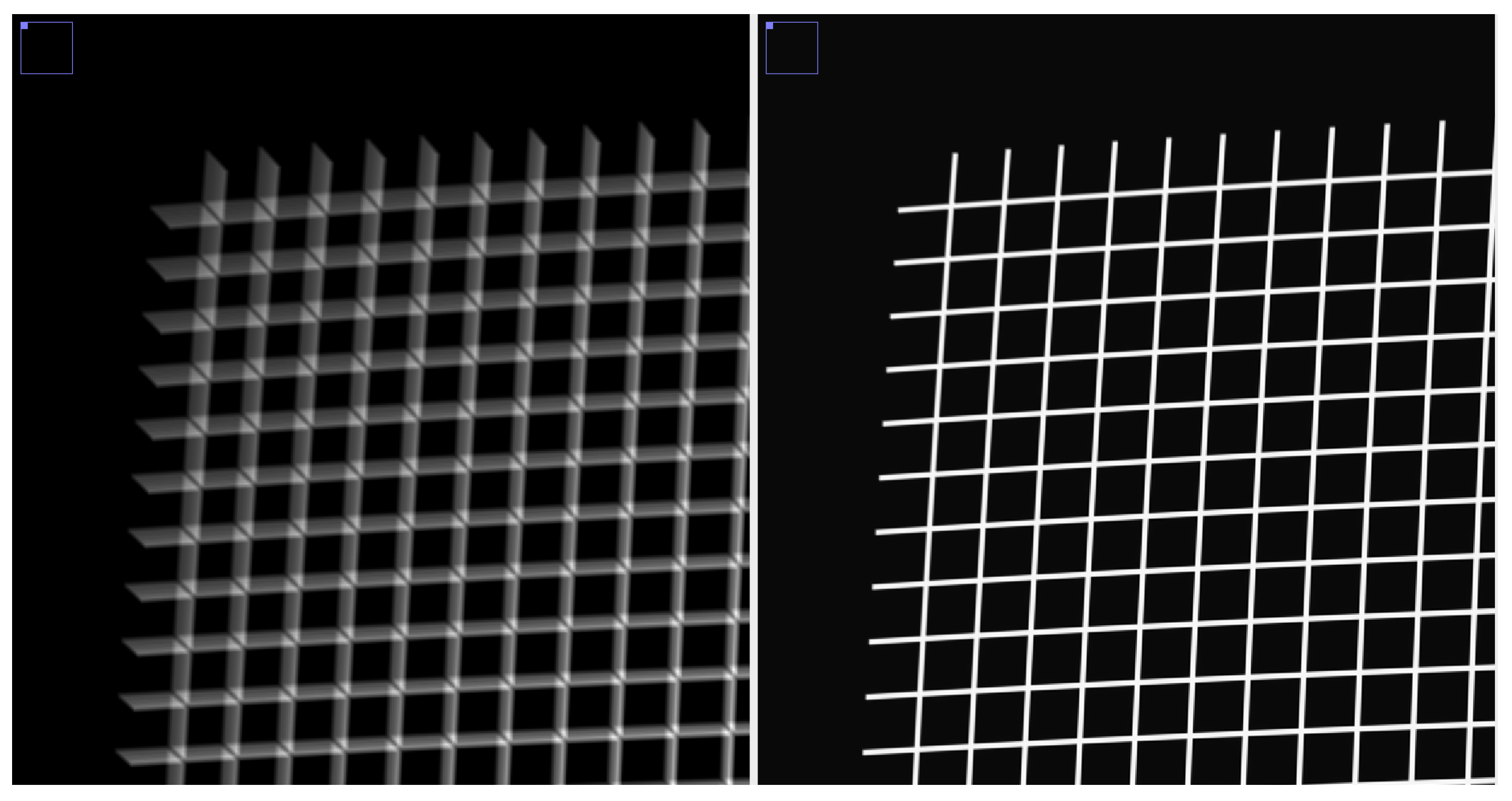
Figure 3.
Phantom movie (grid, detail), an average of 50 frames, frames shifted + doming applied, using only global alignment (left), after local alignment (right).
Figure 3.
Phantom movie (grid, detail), an average of 50 frames, frames shifted + doming applied, using only global alignment (left), after local alignment (right).
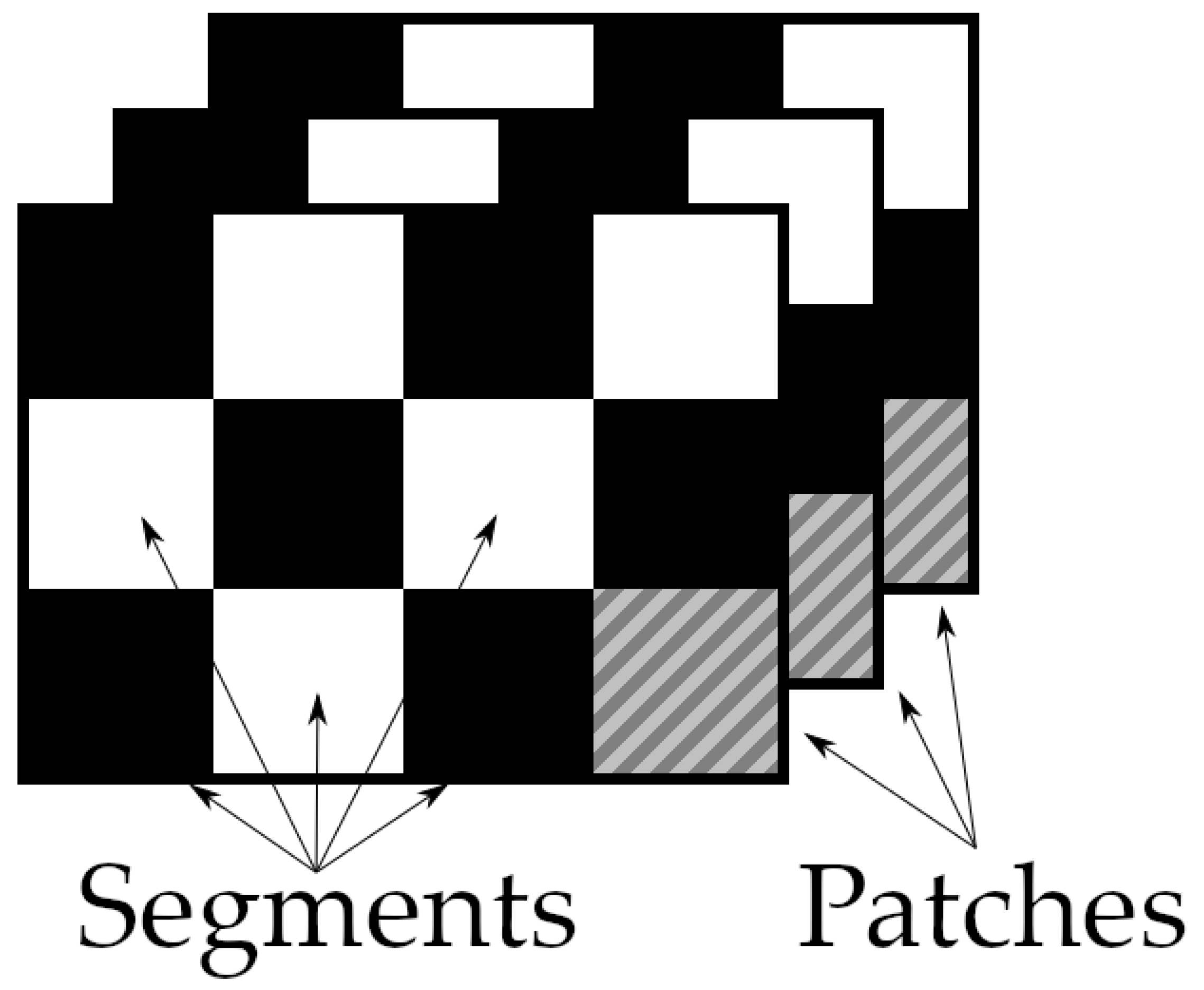
Figure 4.
Division of the frames to patches for local alignment.
Figure 4.
Division of the frames to patches for local alignment.
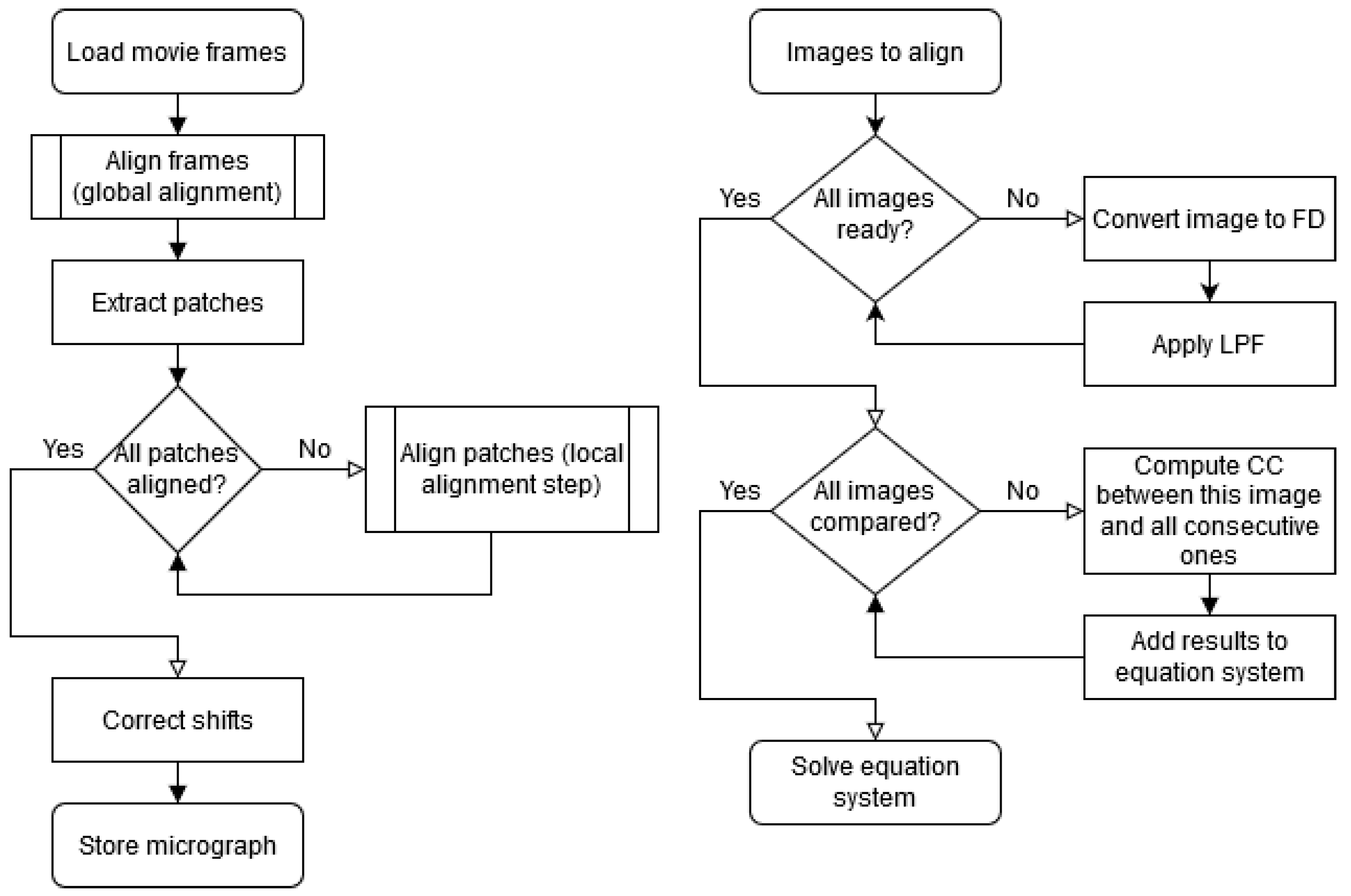
Figure 5.
Flowchart of the core idea of the algorithm. Algorithm overview (left), alignment subroutine (right).
Figure 5.
Flowchart of the core idea of the algorithm. Algorithm overview (left), alignment subroutine (right).
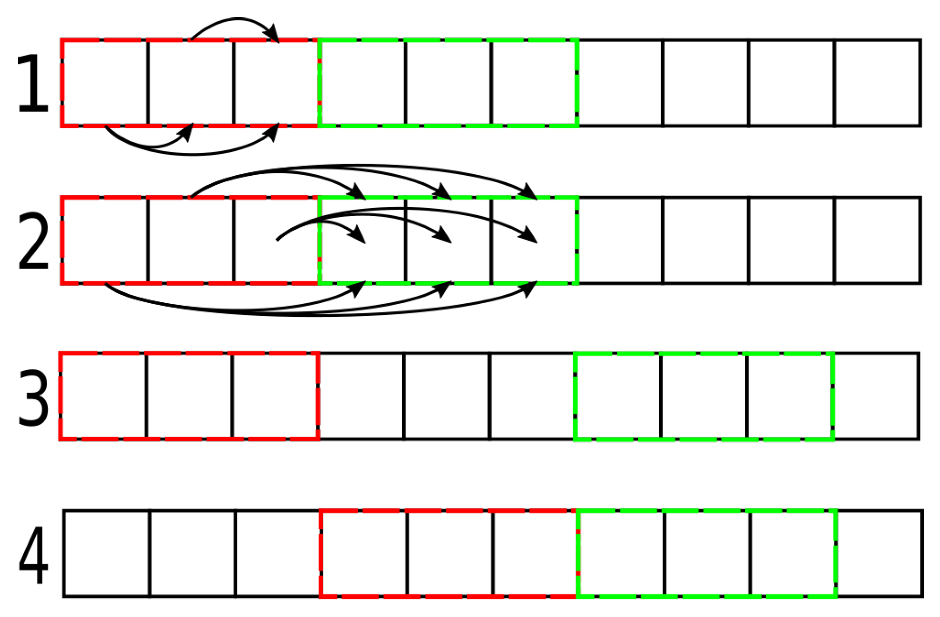
Figure 6.
Data processing using two buffers. First, we process images in the first (red) buffer (1), then all pairs of images in both buffers (2). We iteratively fill the second (green) buffer with remaining images (3, arrows skipped for brevity). When all images pairs for the first buffer are processed, we load new images into the first buffer (4).
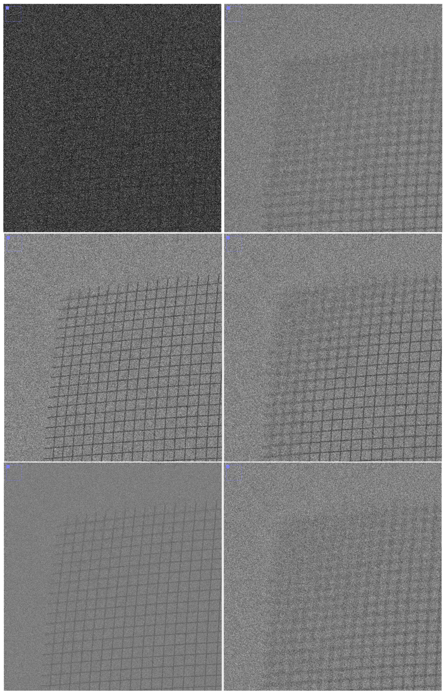
Figure 7.
Detail of the frame of the phantom movie (top left), detail of produced micrograph, normalized: cryoSPARC (top right), FlexAlign (center left), Warp (center right), MotionCor2 (bottom left), Relion MotionCor (bottom right).
Figure 7.
Detail of the frame of the phantom movie (top left), detail of produced micrograph, normalized: cryoSPARC (top right), FlexAlign (center left), Warp (center right), MotionCor2 (bottom left), Relion MotionCor (bottom right).
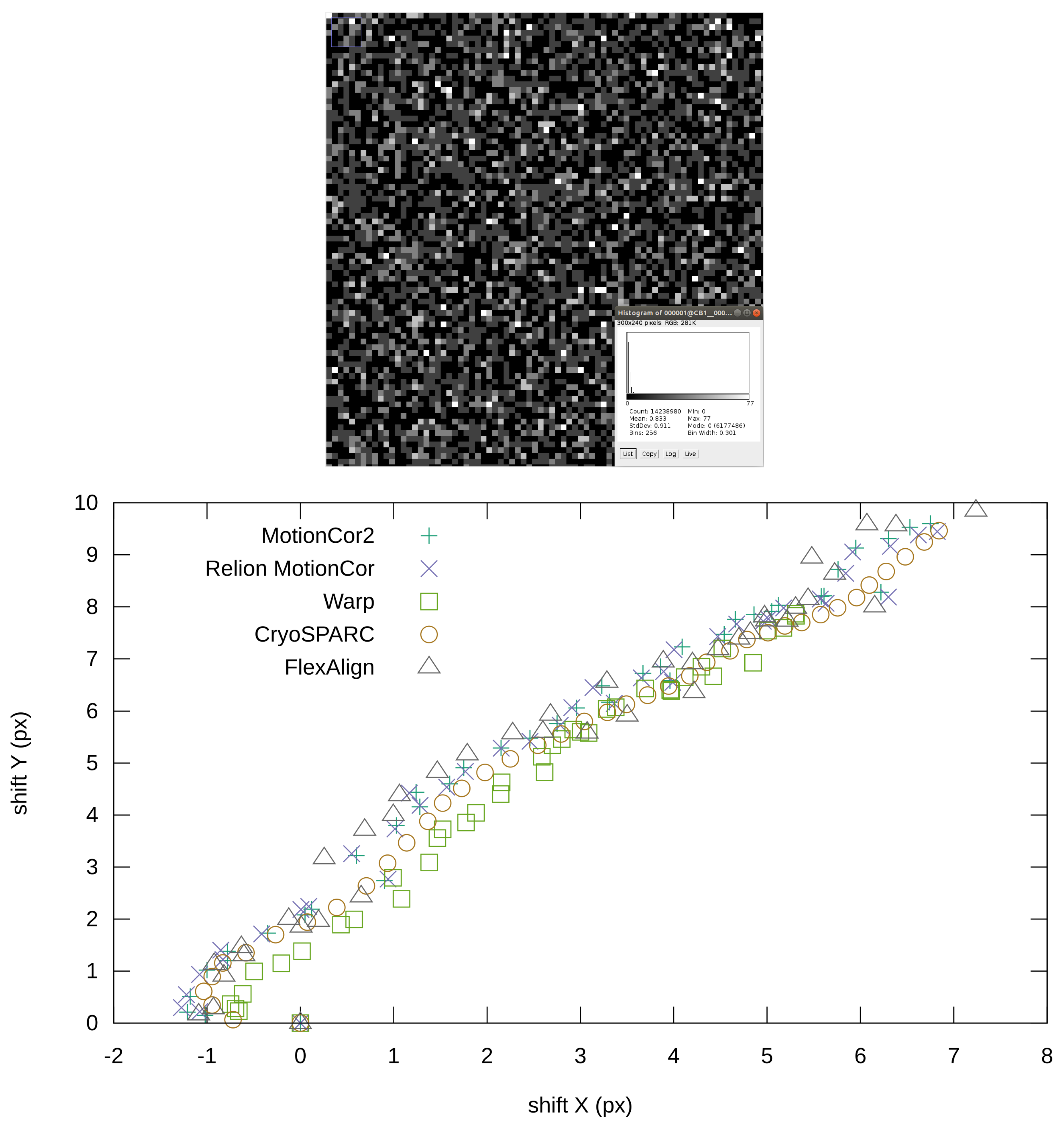
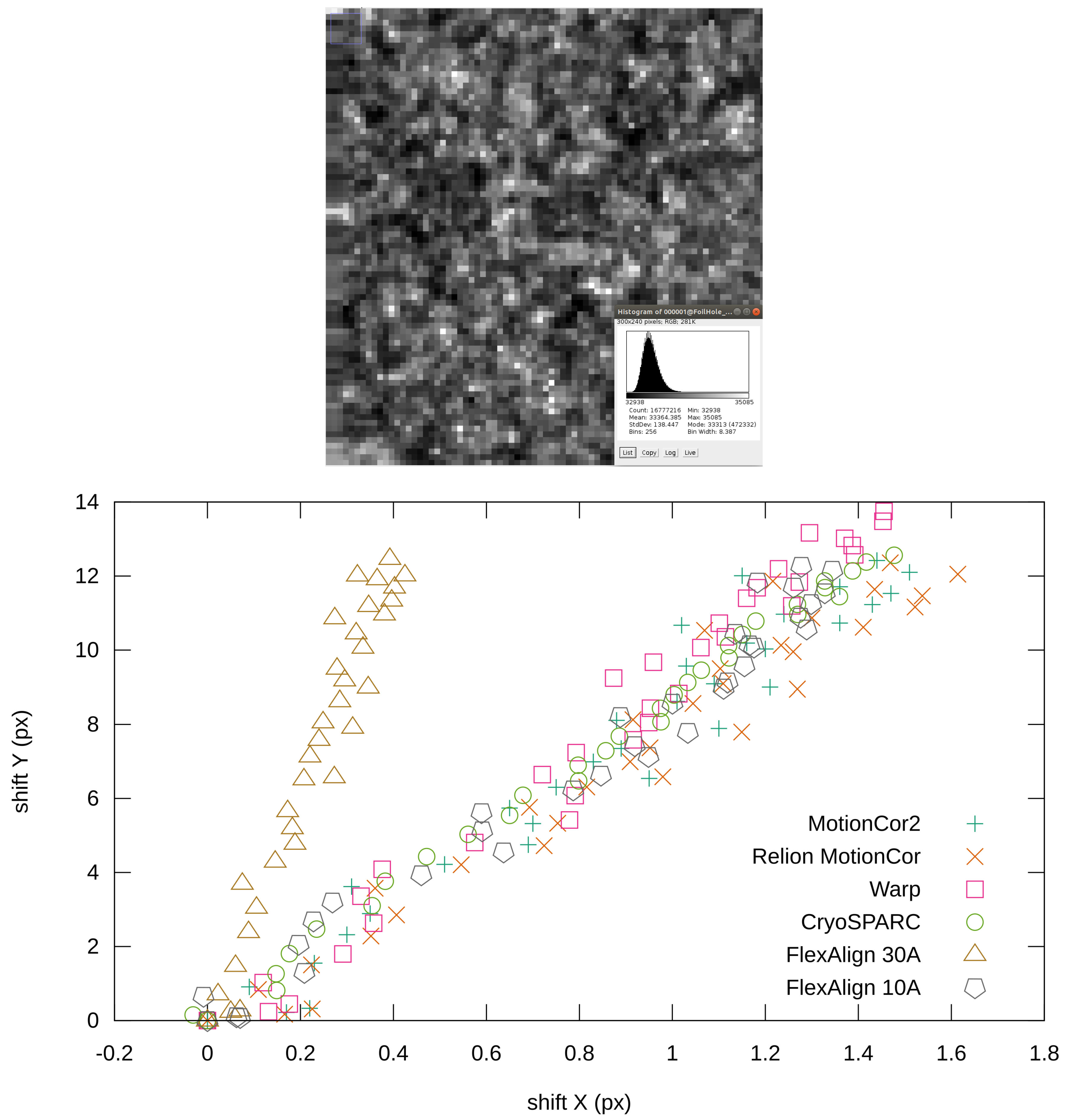
Figure 8.
Detail of the frame from the EMPIAR 10288 (normalized) with histogram (before normalization) (top), reported global shifts by different programs (bottom).
Figure 8.
Detail of the frame from the EMPIAR 10288 (normalized) with histogram (before normalization) (top), reported global shifts by different programs (bottom).
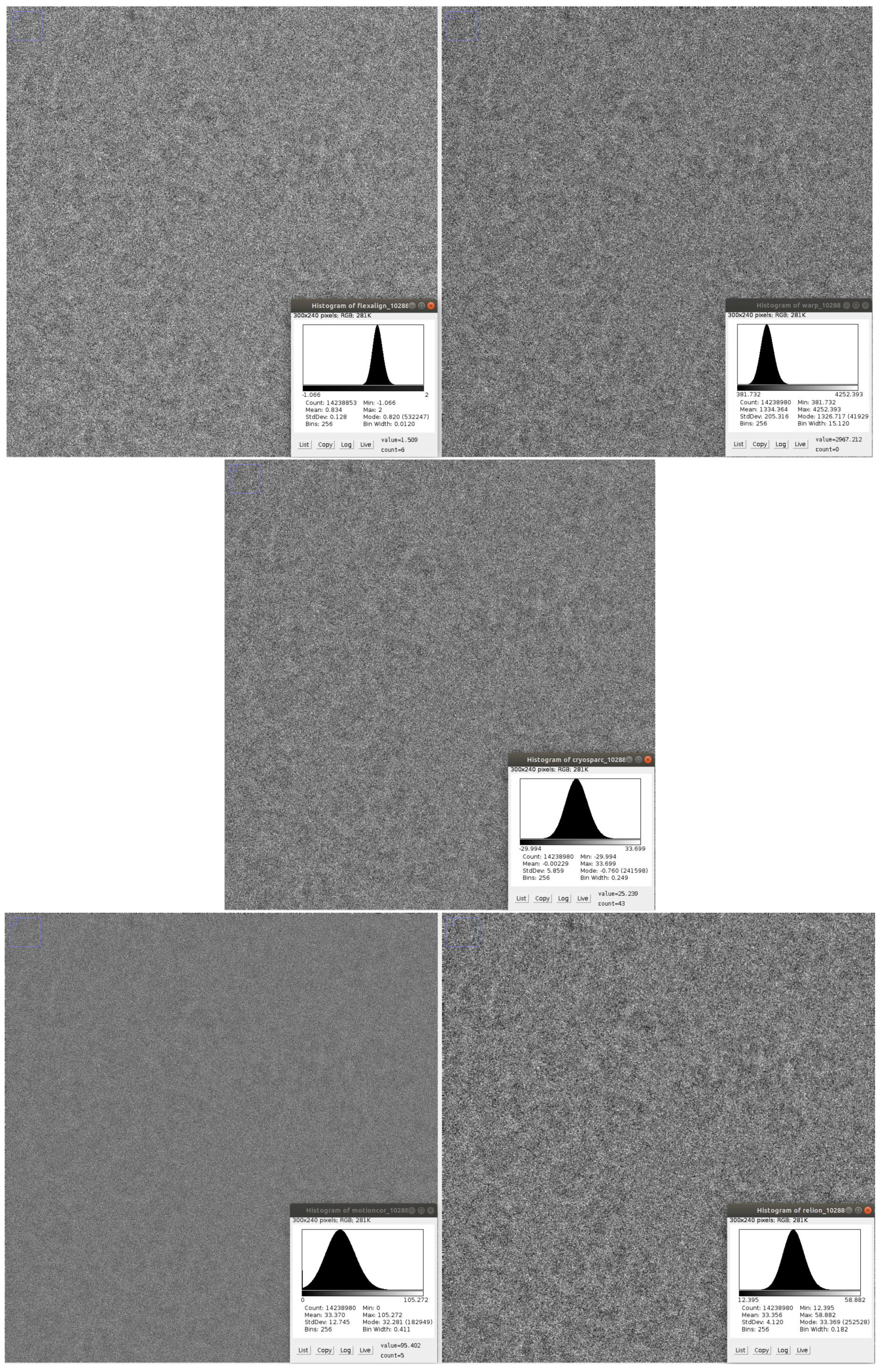
Figure 9.
Detail of the produced micrograph using EMPIAR 10288 dataset (normalized) with histogram (before normalization): FlexAlign (top left), Warp (top right), cryoSPARC (center), MotionCor2 (bottom left), Relion MotionCor (bottom right).
Figure 9.
Detail of the produced micrograph using EMPIAR 10288 dataset (normalized) with histogram (before normalization): FlexAlign (top left), Warp (top right), cryoSPARC (center), MotionCor2 (bottom left), Relion MotionCor (bottom right).
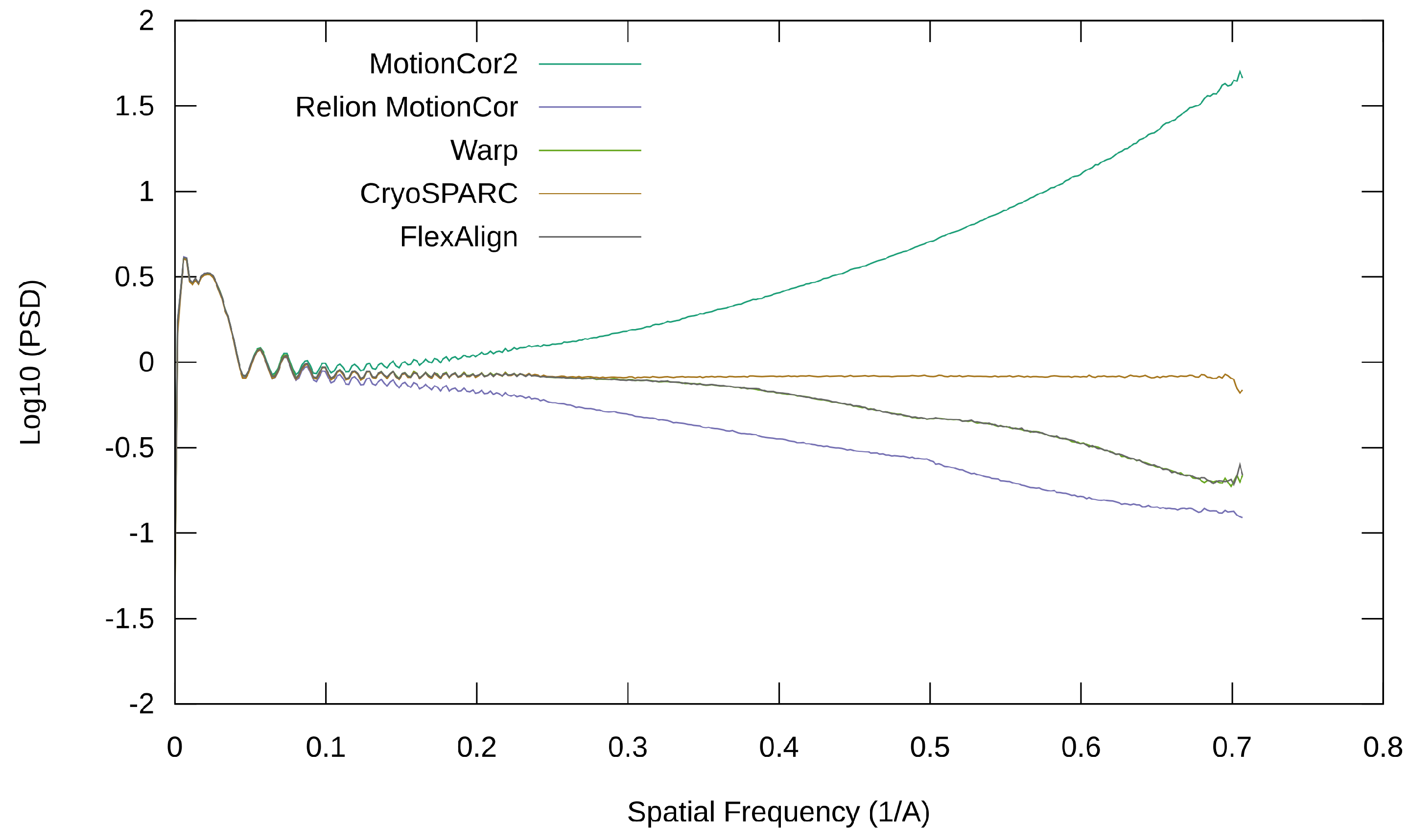
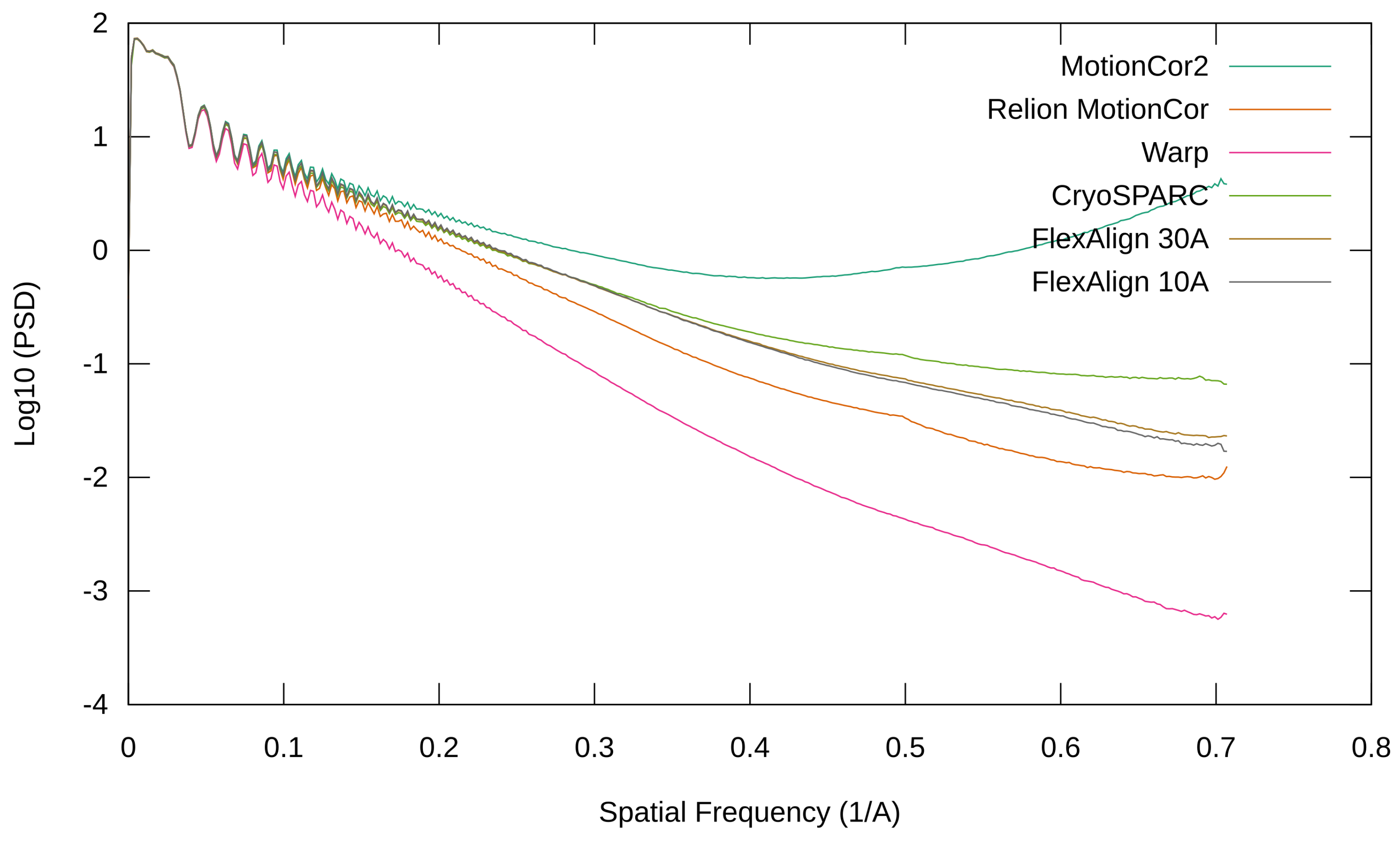
Figure 10.
Radial average of the PSD of the produced micrograph using EMPIAR 10288.
Figure 10.
Radial average of the PSD of the produced micrograph using EMPIAR 10288.
Figure 11.
Details of the frame from the EMPIAR 10314 (normalized) with histogram (before normalization) (top), reported global shifts by different programs (bottom).
Figure 11.
Details of the frame from the EMPIAR 10314 (normalized) with histogram (before normalization) (top), reported global shifts by different programs (bottom).
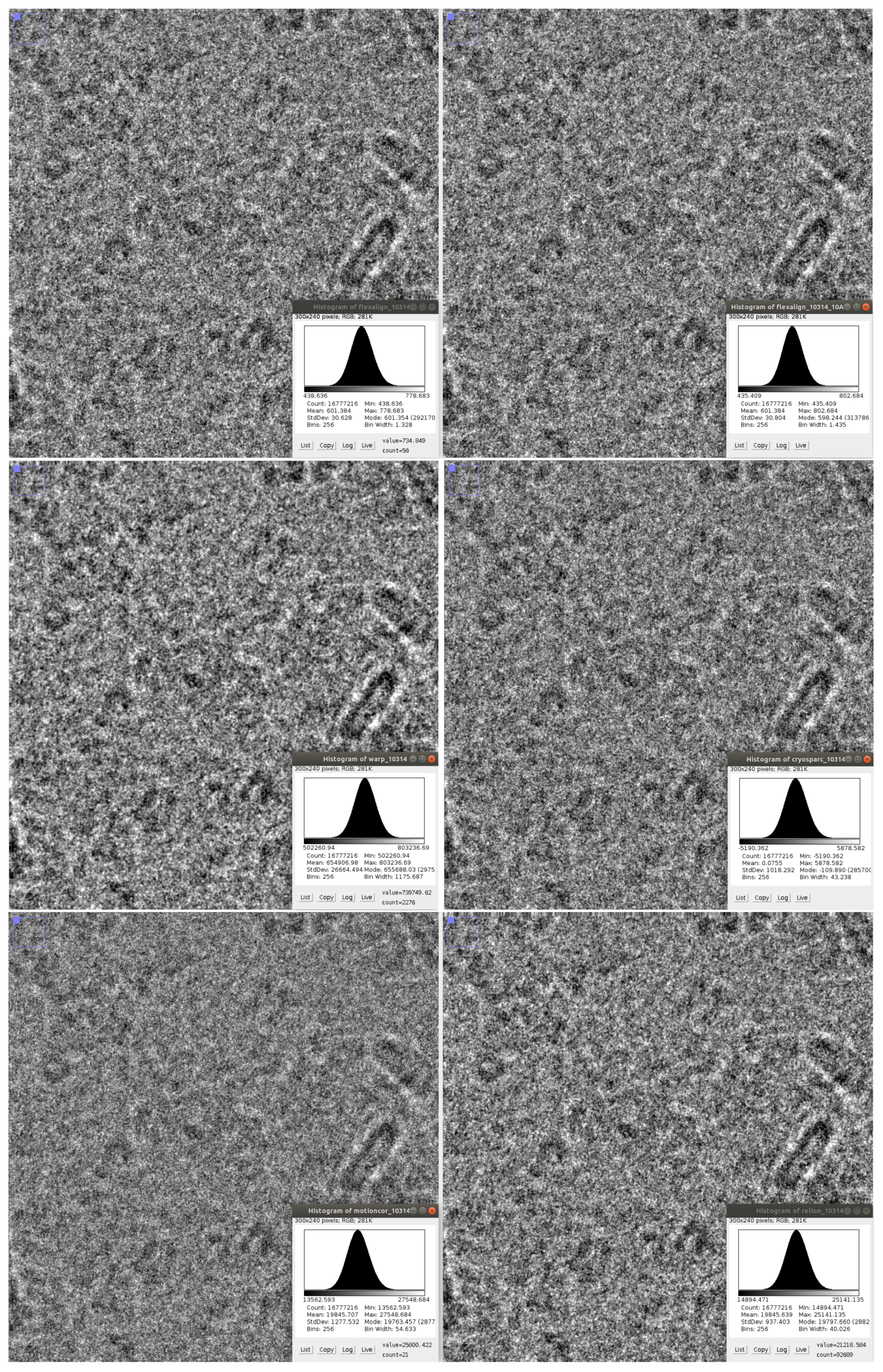
Figure 12.
Details of the produced micrograph using EMPIAR 10314 dataset (normalized) with histogram (before normalization): FlexAlign (top left), FlexAlign with low-pass filter at 10 Å (top right), Warp (center left), cryoSPARC (center right), MotionCor2 (bottom left), Relion MotionCor (bottom right).
Figure 13.
Radial average of the PSD of the produced micrograph using EMPIAR 10314.
Figure 13.
Radial average of the PSD of the produced micrograph using EMPIAR 10314.
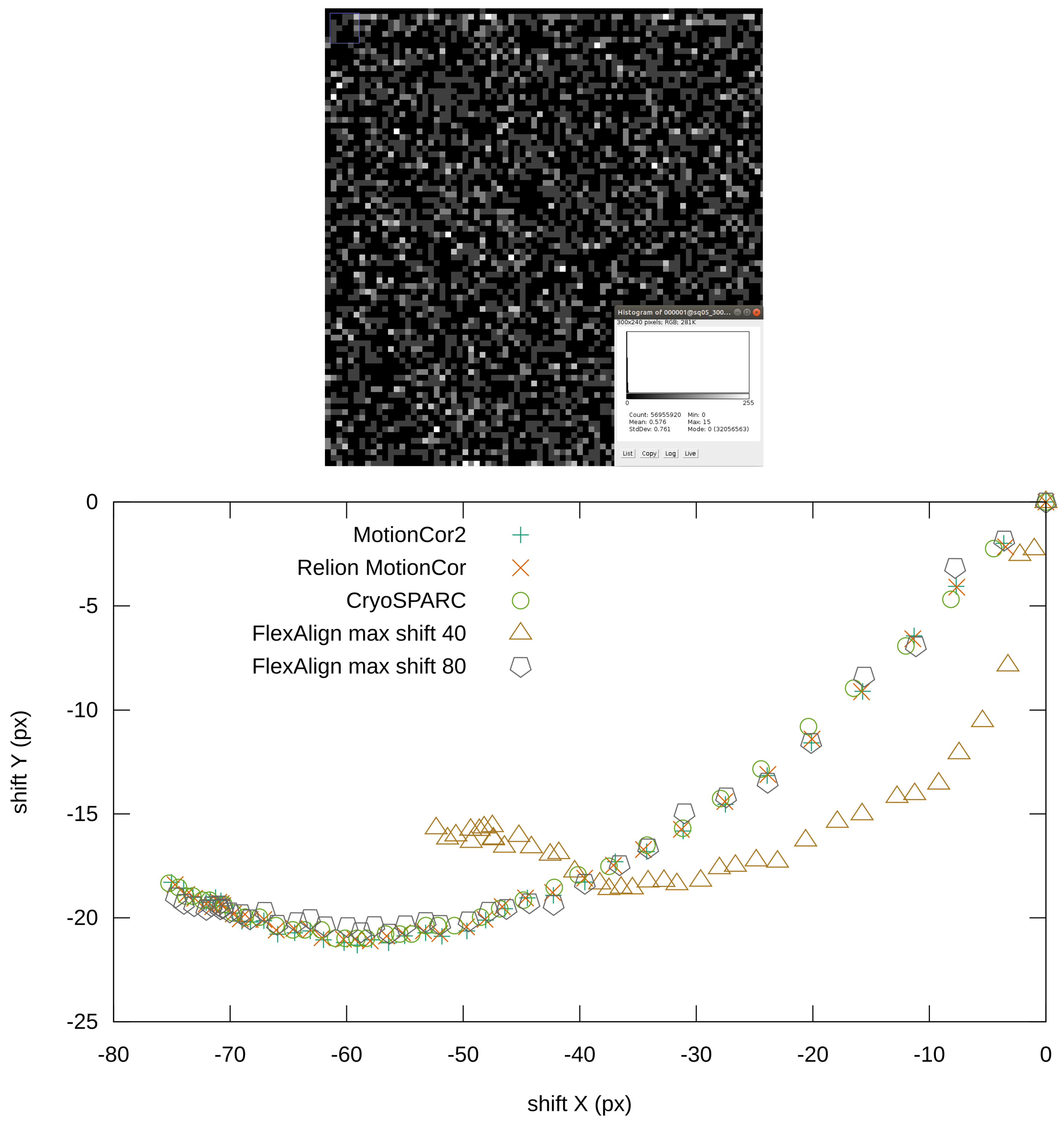
Figure 14.
Details of the frame from the EMPIAR 10196 (normalized) with histogram (before normalization) (top), reported global shifts by different programs (bottom).
Figure 14.
Details of the frame from the EMPIAR 10196 (normalized) with histogram (before normalization) (top), reported global shifts by different programs (bottom).
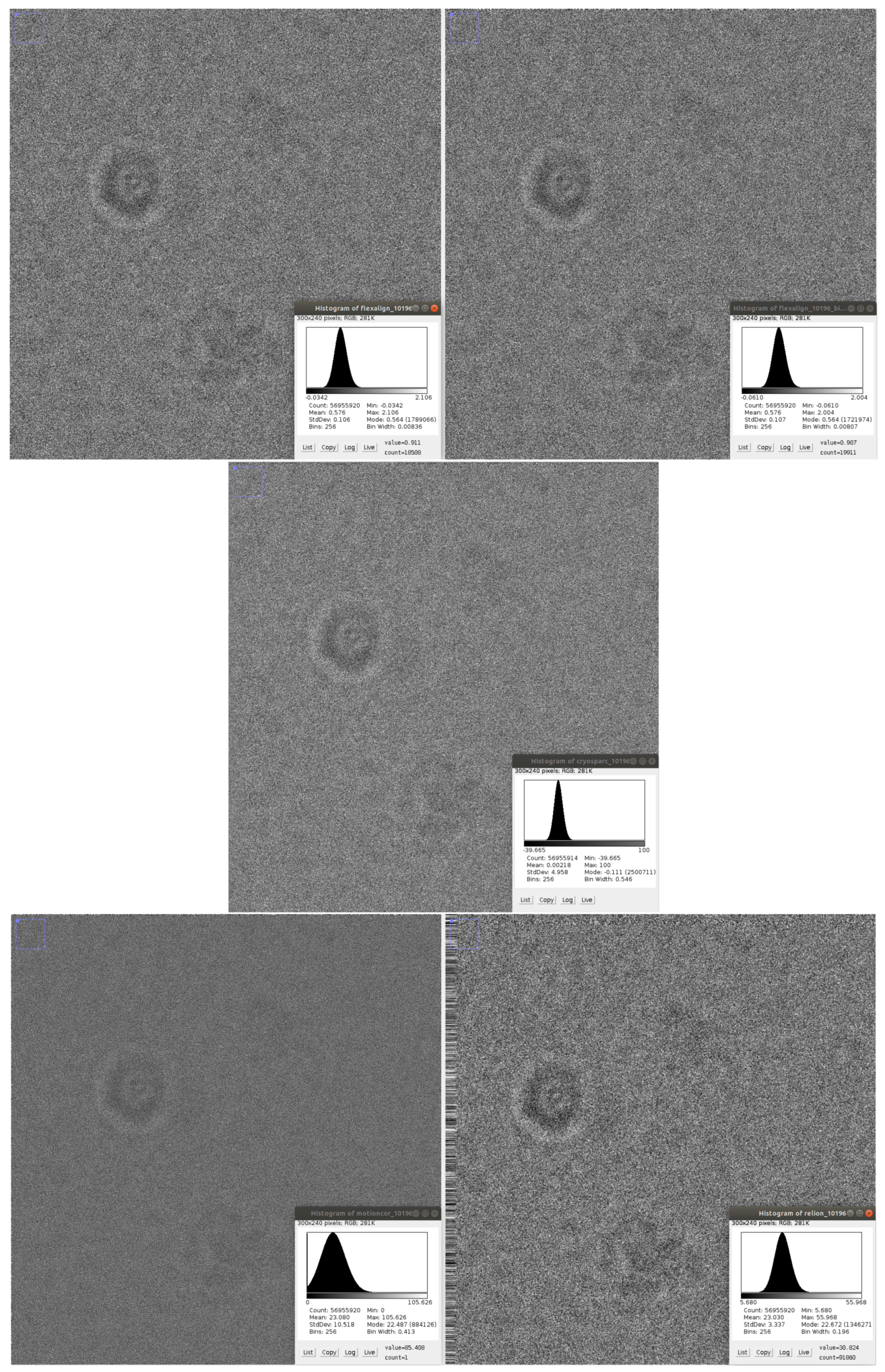
Figure 15.
Details of the produced micrograph using EMPIAR 10196 dataset (normalized) with histogram (before normalization): FlexAlign (top left), FlexAlign with max shift of 80 px (top right), cryoSPARC (center), MotionCor2 (bottom left), Relion MotionCor (bottom right).
Figure 15.
Details of the produced micrograph using EMPIAR 10196 dataset (normalized) with histogram (before normalization): FlexAlign (top left), FlexAlign with max shift of 80 px (top right), cryoSPARC (center), MotionCor2 (bottom left), Relion MotionCor (bottom right).
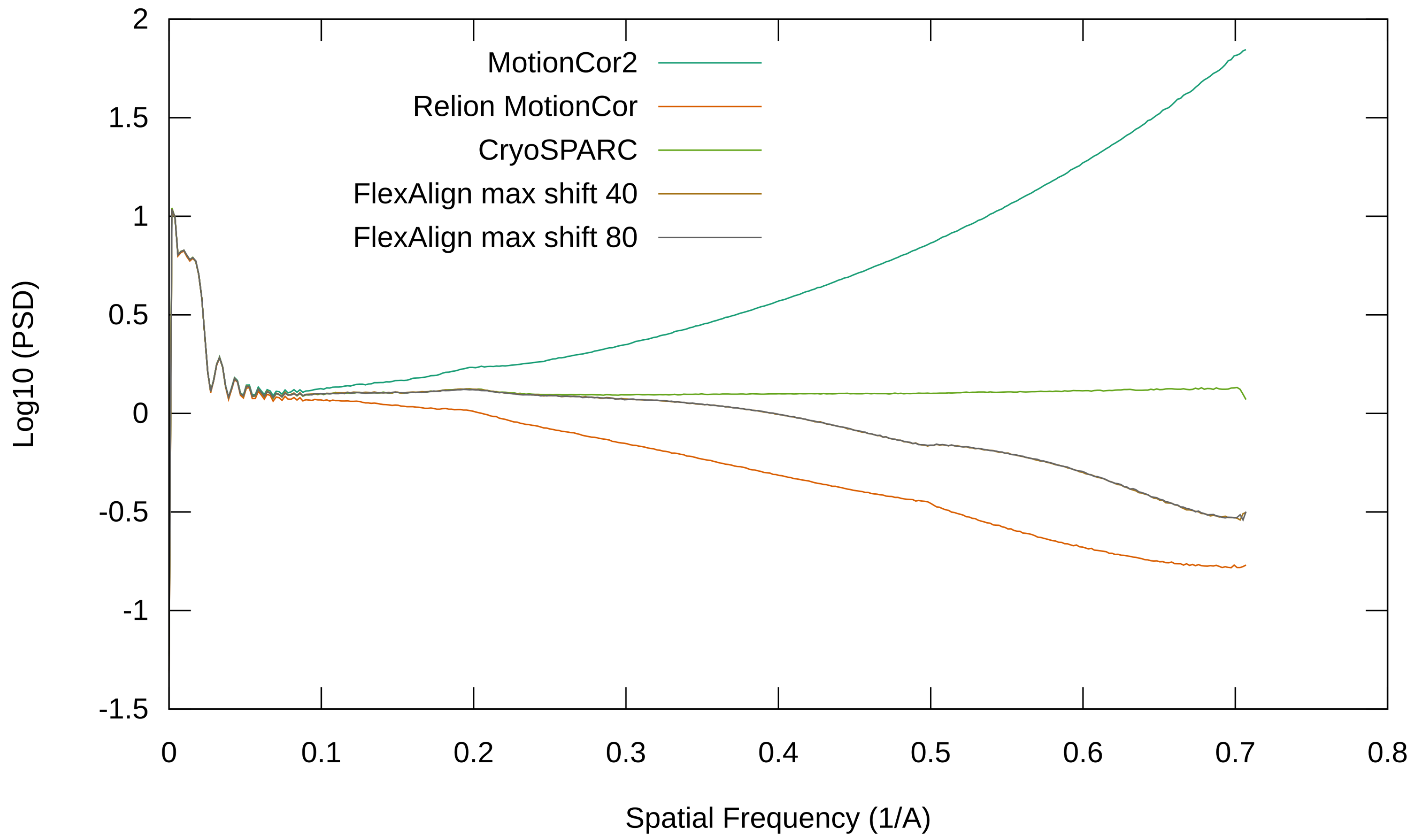
Figure 16.
Radial average of the PSD of the produced micrograph using EMPIAR 10196.
Figure 16.
Radial average of the PSD of the produced micrograph using EMPIAR 10196.
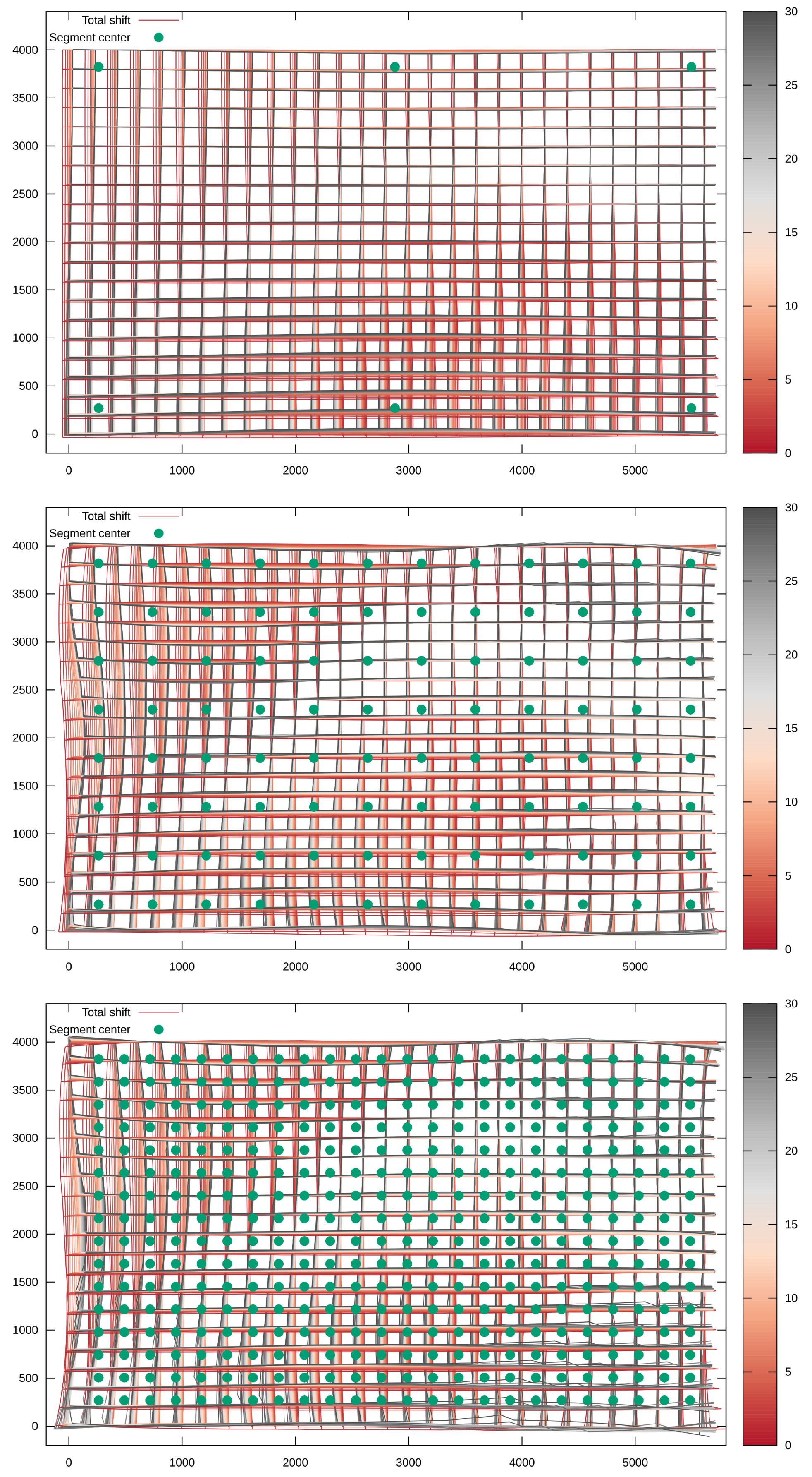
Figure 17.
Influence on shift estimation using a different number of patches: 3 × 2 (top), 12 × 8 (middle, default value), 24 × 16 (bottom).
Figure 17.
Influence on shift estimation using a different number of patches: 3 × 2 (top), 12 × 8 (middle, default value), 24 × 16 (bottom).
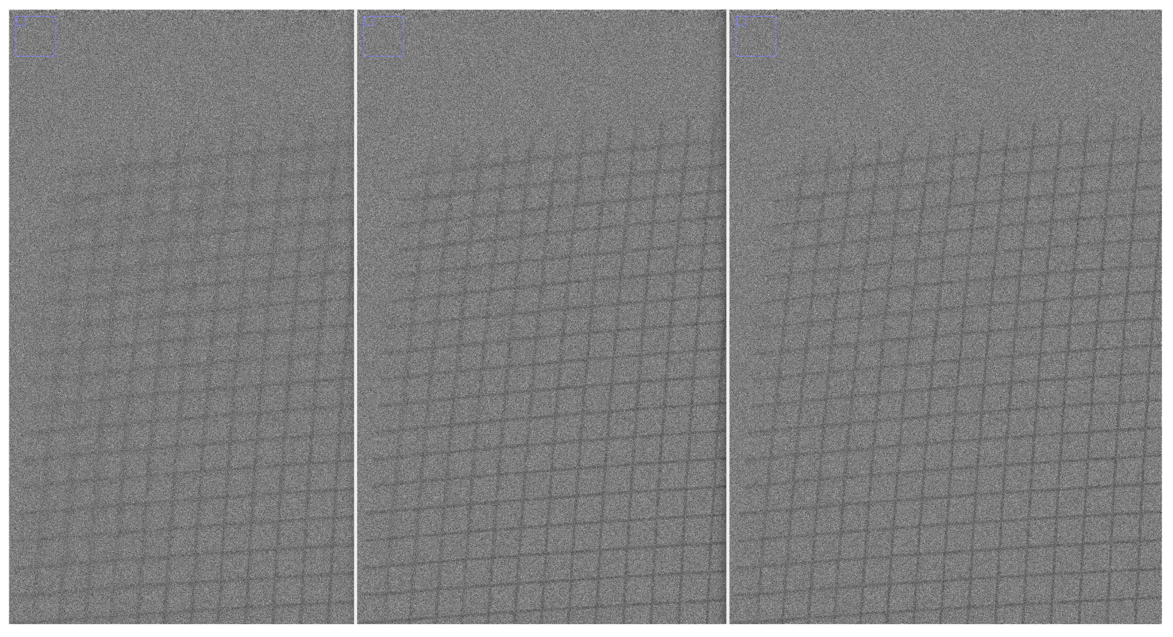
Figure 18.
Normalized micrograph of the phantom movie produced by MotionCor2, using different number of patches: 5 × 5 (left), 7 × 7 (middle), 9 × 9 (right).
Figure 18.
Normalized micrograph of the phantom movie produced by MotionCor2, using different number of patches: 5 × 5 (left), 7 × 7 (middle), 9 × 9 (right).
Table 1.
Comparison of various movie alignment algorithms.
Table 1.
Comparison of various movie alignment algorithms.
| Program | HW | Method + Interpolation |
|---|
| MotionCor2 | GPU | CC + polynomial |
| Relion MotionCor | CPU | CC + polynomial |
| Optical flow | CPU/GPU | optical flow + cubic interpolation |
| Warp | GPU | CC + higher-order schemes |
| FlexAlign | GPU | CC + B-spline |
Table 2.
HW used for benchmarking.
Table 2.
HW used for benchmarking.
| | Testbed 1 | Testbed 2 | Testbed 3 |
|---|
| CPU | Intel(R) Core(TM) i7-8700 (12 cores, 3.20 GHz) | Intel(R) Core(TM) i7-7700HQ (4 cores, 2.80 GHz) |
| GPU | GeForce RTX 2080 | GeForce GTX 1070 | GeForce GTX 1060 |
| CUDA/driver | 10.1/418.39 | 10.1/418.67 | 8.0.61/436.02 (Win 10)/390.116 (Ubuntu 18.04) |
| SSD | Samsung SSD 970 EVO 500 GB | NVMe TOSHIBA 1024 GB |
| RAM | 2 × 16 GB DDR4 @ 2.6 GHz | 2 × 16 GB DDR4 @ 2.4 GHz |
Table 3.
Resolution and number of frames used for testing.
Table 3.
Resolution and number of frames used for testing.
| | Size | No. of Patches |
|---|
| Falcon | 4096 × 4096 × 40 | 9 × 9 |
| K2 | 3838 × 3710 × 40 | 8 × 8 |
| K2 super (resolution) | 7676 × 7420 × 40 | 16 × 15 |
| K3 | 5760 × 4092 × 30 | 12 × 9 |
| K3 super (resolution) | 11,520 × 8184 × 20 | 24 × 17 |
Table 4.
Execution time on Testbed 1.
Table 4.
Execution time on Testbed 1.
| | Falcon | K2 | K2 Super | K3 | K3 Super |
|---|
| MotionCor2 | 4.6 s | 4.3 s | 15.7 s | 5.0 s | 13.1 s |
| FlexAlign (tuned) | 9.2 s | 7.6 s | 25.6 s | 8.8 s | 20.5 s |
| FlexAlign (autotuning) | 49.2 s | 34.4 s | 71.9 s | 59.3 s | 72.2 s |
| FlexAlign (non-tuned) | 10.8 s | 9.1 s | 31.5 s | 10.7 s | 22.9 s |
| Movies to pay-off | 25 | 18 | 8 | 27 | 22 |
Table 5.
Execution time on Testbed 2.
Table 5.
Execution time on Testbed 2.
| | Falcon | K2 | K2 Super | K3 | K3 Super |
|---|
| MotionCor2 | 5.5 s | 5.2 s | 20.3 s | 5.9 s | 15.7 s |
| FlexAlign (tuned) | 9.0 s | 8.2 s | 27.3 s | 9.3 s | 21.1 s |
| FlexAlign (autotuning) | 47.8 s | 38.7 s | 73.3 s | 56.2 s | 65.7 s |
| FlexAlign (non-tuned) | 11.7 s | 10.4 s | 35.2 s | 11.5 s | 26.9 s |
| Movies to pay-off | 15 | 14 | 6 | 22 | 8 |
Table 6.
Execution time on Testbed 3.
Table 6.
Execution time on Testbed 3.
| | Falcon | K2 | K2 Super | K3 | K3 Super |
|---|
| Warp | 11.7 s | 10 s | 14.2 s | 13.1 s | 15.6 s |
| FlexAlign (tuned) | 11.9 s | 9.9 s | 35.5 s | 11.3 s | 27.7 s |

 ,
, 


