Article

Modeling and Control of the Starter Motor and Start-Up Phase for Gas Turbines

by
Soheil Jafari
1,*,
Seyed Alireza Miran Fashandi
2 and
Theoklis Nikolaidis
3
1
Propulsion Engineering Centre, School of Aerospace Transport and Manufacturing, Cranfield University, Cranfield MK43 0AL, UK
2
Department of Mechanical Engineering, Iran University of Science and Technology, Tehran 16846-13114, Iran
3
Propulsion Engineering Centre, School of Aerospace Transport and Manufacturing, Cranfield University, Cranfield MK43 0AL, UK
*
Author to whom correspondence should be addressed.
Electronics 2019, 8(3), 363; https://doi.org/10.3390/electronics8030363
Submission received: 18 February 2019 / Revised: 14 March 2019 / Accepted: 19 March 2019 / Published: 25 March 2019
(This article belongs to the Section Systems & Control Engineering)

Abstract

:
Improving the performance of industrial gas turbines has always been at the focus of attention of researchers and manufacturers. Nowadays, the operating environment of gas turbines has been transformed significantly respect to the very fast growth of renewable electricity generation where gas turbines should provide a safe, reliable, fast, and flexible transient operation to support their renewable partners. So, having a reliable tools to predict the transient behavior of the gas turbine is becoming more and more important. Regarding the response time and flexibility, improving the turbine performance during the start-up phase is an important issue that should be taken into account by the turbine manufacturers. To analyze the turbine performance during the start-up phase and to implement novel ideas so as to improve its performance, modeling, and simulation of an industrial gas turbine during cold start-up phase is investigated this article using an integrated modular approach. During this phase, a complex mechatronic system comprised of an asynchronous AC motor (electric starter), static frequency converter drive, and gas turbine exists. The start-up phase happens in this manner: first, the clutch transfers the torque generated by the electric starter to the gas turbine so that the turbine reaches a specific speed (cranking stage). Next, the turbine spends some time at this speed (purging stage), after which the turbine speed decreases, sparking stage begins, and the turbine enters the warm start-up phase. It is, however, possible that the start-up process fails at an intermediate stage. Such unsuccessful start-ups can be caused by turbine vibrations, the increase in the gradients of exhaust gases, or issues with fuel spray nozzles. If, for any reason, the turbine cannot reach the self-sustained speed and the speed falls below a certain threshold, the clutch engages once again with the turbine shaft and the start-up process is repeated. Consequently, when modeling the start-up phase, we face discontinuities in performance and a system with variable structure owing to the existence of clutch. Modeling the start-up phase, which happens to exist in many different fields including electric and mechanical application, brings about problems in numerical solutions (such as algebraic loop). Accordingly, this study attempts to benefit from the bond graph approach (as a powerful physical modeling approach) to model such a mechatronic system. The results confirm the effectiveness of the proposed approach in detailed performance prediction of the gas turbine in start-up phase.

1. Introduction

Current focuses of industrial gas turbine manufacturers are on minimizing costs, enhancing flexibility and capacity, while retaining the reliability. This has motivated well-known companies including Siemens [1], GE [2], and Alstom [3] to work on a set of what is known as performance enhancement methods to be able to yield more profit.
In order to increase the flexibility of industrial gas turbine, improving the start-up phase is of considerable importance since the start-up phase in most utilized gas turbines has created challenges in gas transmission line stations in certain countries, resulting in trip in the turbine [4]. The reason behind such unsuccessful start-ups could be attributed to turbine vibrations, the increase in the gradients of exhaust gases, or problems in fuel spray nozzles. If the turbine is unable to attain the self-sustained speed and its speed falls below a certain limit, the clutch engages with the turbine shaft once more and the start-up process is repeated. This in turn increases the turbine start-up duration and incurs expenses for repair and maintenance. Therefore, appropriately performing the start-up process and reducing its time have always been considered by manufacturers. Since the performance of the gas turbine during the start-up phase has direct impacts on its lifespan as well as the time required for its repair, the importance of this notion becomes much more significant. For instance, Siemens believes that as the market continues to grow, faster start-ups become as important as recurring ones. As a result, Siemens launched a project named FACY, abbreviated from fast cycling (Figure 1), to integrate every engineering thought into a comprehensive plant concept. The purpose was to devise a plant that could increase the frequency of starts while decreasing their duration and keeping the requirements of other components to a minimum including the steam generator used for heat recovery at warm and hot start-ups [4].
Additionally, investigation and implementation of improving the performance of start-up phase were carried out by GE company researchers. For instance, the start-up phase of a normal industrial gas turbine, GE LM6000, which takes 10 min is displayed in Figure 2.
The start-up phase of the GE LM6000 industrial gas turbine is reduced to less than 5 min by implementing the following actions (Figure 3 shows the new start-up process of this gas turbine):
  • No LLP (Life Limited Parts) penalty when used less than 4 times a year
  • Two cycles per 1 penalty when used more than 4 times a year
  • Observation and measurement manual should be checked when used more than 4 times a year.
In general, the start-up phase of an industrial gas turbine can be divided into two phases of cold and warm start-ups. During cold start-up phase, the turbine is first accelerated using a starter (usually electric starter) and reaches a certain rpm (cranking stage), then spends some time at this rpm (purging stage). Next, rpm is reduced and sparking and combustion stage begins. This is when the warm start-up phase commences. These stages are shown in Figure 2 and Figure 3 as an example.
So, as it is clear from Figure 2 and Figure 3, the performance of the start-up phase is improved in the following stages. In addition, as shown in the figures, the first two stages occur during the cold start-up phase:
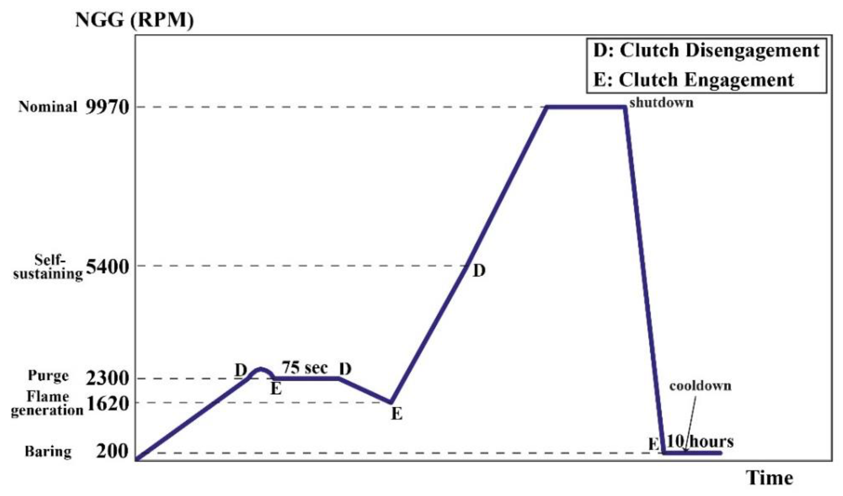
  • Initialization, purge of enclosure
  • Purge of engine/stack
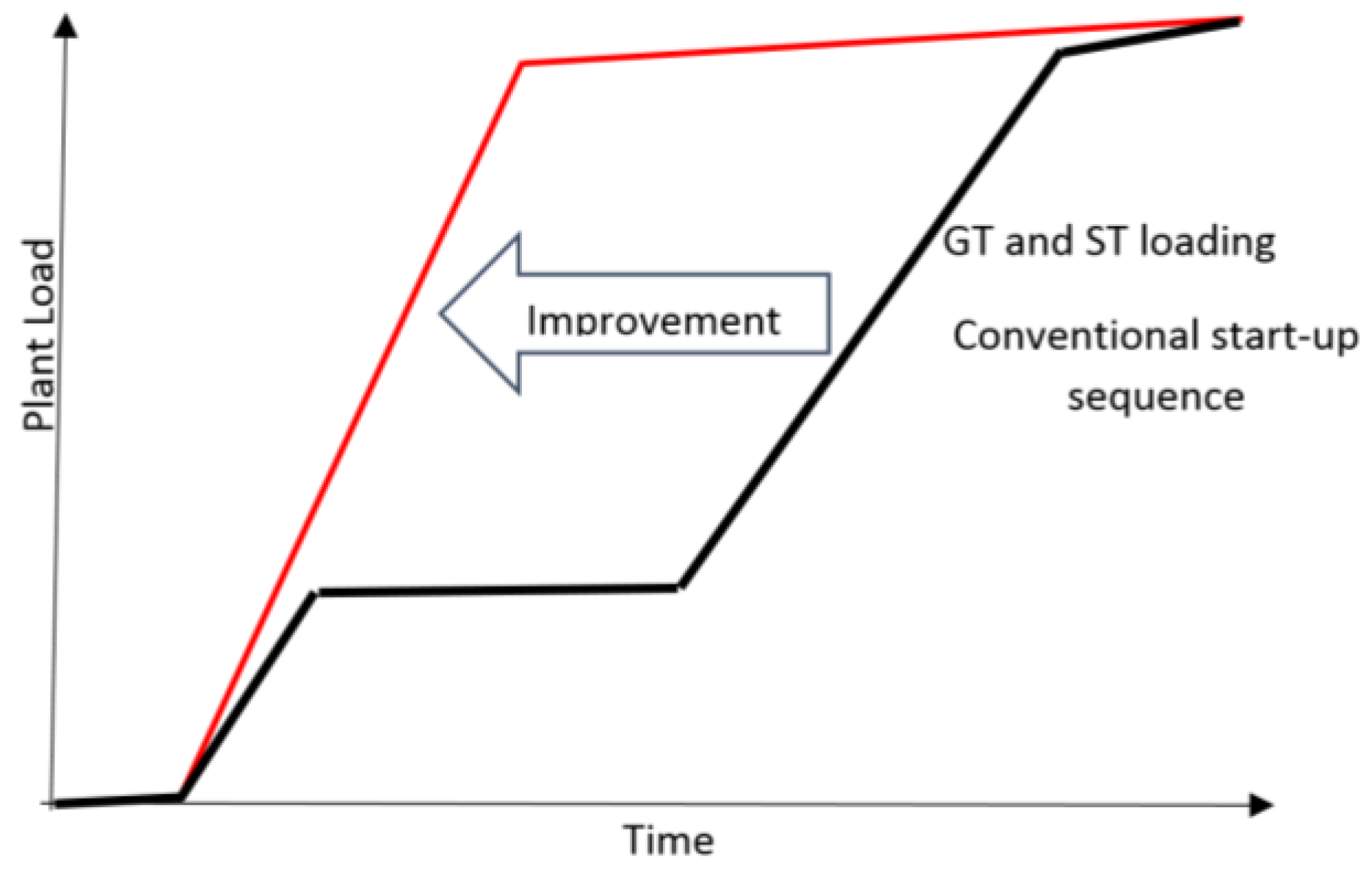
  • Acceleration to reach sync idle
  • Synchronization to grid, then warm up
  • Acceleration to reach full load
In most industrial gas turbines, including the studied one in this research, active components in the cold start-up phase include asynchronous AC motor and static frequency converter (SFC) to control the induction motor and clutch as shown in Figure 4.
To analyze and improve the performance of gas turbine during start-up phase, modeling and simulation of turbine are required in addition to experimental investigation. The designer gains a better insight on the system using numerical simulation so as to apply modifications and experiment with the system response in the easiest manner. In other words, simulation is what connects the design to operation. However, certain challenges still exist when simulating and modeling the cold start-up phase of industrial gas turbines as various energy fields such electric and mechanical areas have energy and information interaction. This results in specific numerical issues such as the occurrence of algebraic loop in conventional software including Matlab. Overall, numerical stiffness issues caused by discontinuity and systems variable-structure systems make the simulation and modeling of such systems a cumbersome task.
Poluéktova [6] presented a mathematical model for a special gas-turbine unit named DYa-95l accompanied by a free power turbine. Using this model, the emergency operation of a gas-turbine as well as its start-up process were studied in an efficient manner. Simulations for determining the parameters of automatic start-up alternatives were also performed. Bahlawan et al. [7] considered a General Electric PG 9351FA gas turbine and studied setting up reliable Nonlinear Autoregressive Exogenous (NARX) models with the aid of sensitivity analysis. They also defined a novel performance function for better analysis of quick transients and could design an accurate and efficient tool for simulations that could also be used for diagnosis of gas turbines. Asgari et al. [8] performed a series of studies on the start-up phase of a heavy-duty industrial gas turbine using neural network approach implemented in MATLAB. Both NARX and Simulink models were capable of appropriate prediction but not the turbine behavior during the cold start-up phase. Using a physics-based model, Morini et al. [9] attempted to study a single-shaft gas turbine especially during the start-up phase. The proposed model could consider both steady-state and dynamic characteristics using shaft power balance along with other features such as considering heat soakage. They finally tested ALSTOM GT13E2 gas turbine to validate their proposed model. Regarding novelty detection in industrial gas turbines, Zhang et al. [10] focused on analyzing start-up vibration. To this end, a vibration signature obtained from accurate measurements based on a neuro-fuzzy system was necessary. They could detect conditions of novel/fault during start-up along with cross-correlation measures and Euclidean distance.
Mahdipour and Bathaee [11] designed a new SFC based on a 7-level voltage source inverter to provide the capability of start-up of whole similar units in a Tehran power plant with a single SFC. The inverter switching frequency was lower than that of other classical methods, whereas the total harmonic distortion of the machine current was under 6%. The simulation results confirmed the functionality of proposed system during shutdown and start-up. In another study by An et al., [12] a novel senseless start-up method along with a flux estimator were designed. Utilizing a phase locked loop, they could obtain the rotor speed to a good accuracy in addition to precise estimation of initial rotor angle. Their load commutated inverter (LCI) system was designed based on a closed loop method, while Simpower/Matlab was used in their modeling process to assess the performance of their start-up method. An and Cha [13] could develop a novel start-up method designed for an LCI in a synchronous generator. They could successfully determine the early rotor position in just 150 ms with an error of less than 1%. Simulink was used to model the current controller and the performance of presented method was verified in Psim.
Bretschneider and Reed [14] focused on engine start-up with static engine-off states. In doing so, they benefited from existing turbofan simulations. A case study focusing on the effects of ground starts was added that compared findings from engine dry crank with those of simulations, corroborating the ability of simulation for estimation of proper trends. Sheng et al. [15] employed an inexact computational approach regarding low-speed part behavior in aeroengines so as to obtain comprehensive component characteristics with the aid of integrating empirical data above idle. The result was a turboshaft engine model that could consider the start-up state. The full-range model obtained by a computational approach proved to be of high accuracy. Sukhovii et al. [16] noted the lack of enough research on component maps at sub-idle mode and presented a novel method for simulation of the starting phase that incorporated a linear dynamic model accompanied by a simple static one so that the relations between rotational speed and gas path parameters can be explained in a simplified manner.
Cao et al. [17] devised a speed control arrangement for a heavy-duty gas turbine, accompanied by a Simulink model of the gas turbine with its accompanying control system. A notable finding was that the gas turbine transient response when isolated showed more variation compared to the synchronized case. To tackle the issue of lack of component map data, especially in low rotational speeds, Hu et al. [18] focused on sub-idle modeling to propose a generalized method. To model various accessories along with combustion chamber, they benefited from analytic calculations, and the model accuracy was improved using the coefficients of total pressure loss.
Agrawal and Yunis [19] presented an approximation of gas turbine behavior during start-up phase. As an example study, they presented the characteristic curve of a starter motor accompanied by torque—speed plots at different battery voltages and validated their model using test data of a turbofan, a turboshaft and a turboprop engine. Kim et al. [20] involved in the modeling and simulation of the start-up process of a heavy-duty industrial gas turbine. In their research, they considered the performance of the electric starter during the start-up phase in an approximate manner, but did not propose a relevant model. In addition, they did not consider the purging stage in the cold start-up phase which occurs prior to the combustion stage. Blomstedt et al. [21] considered the challenges for Siemens SGT600 in cold climates as the material used in the start-up may become brittle. Since solutions such as using an electric pre-heater or using less-brittle materials may not be feasible, another novel solution is to incorporate a control logic which can tackle the issue during start-up in the software so that no additional hardware or change in the material is required especially when the temperature falls below −30 °C (−22 °F) by automatically checking the amount of stress prior to loading the machine. Motazeri-Gh and Miran-F [22], investigated the idea of compressed air injection in the cold start-up phase of a microjet engine using bond graph approach. In another research, they focused on modeling of the electric starter of a small jet engine with the aid of bond graph method [23]. They also carried out the simulation and modeling of JetQuad system with the same methodology [23]. The use of NARX model for start-up phase simulation is also investigated in [24].
In renewable energy sector, a system level approach for combined cycle gas turbine start-up phase has been done by utilizing a model-based control approach in [25,26]. Moreover, dynamic performance simulation and control of gas turbine used for hybrid gas/wind energy application has been discussed in detail in [27].
The lack of published articles around the modeling of industrial gas turbines during start-up phase, leads to this conclusion that no study has been performed on the integrated dynamic modeling of the cold start-up phase of industrial gas turbine. An example of improving GE LM6000 industrial gas turbine during cold start-up phase in Figure 2 and Figure 3 demonstrates the importance of investigating this phase. In other words, the duration of engine/stack purge is shown to be 90 s in Figure 2, whereas this time is reduced to 15 s in Figure 3. This stage represents the process of cranking and purging in cold start-up phase. A complicated mechatronic system composed of an asynchronous motor (starter motor), SFC drive, clutch, and gas turbine are contributing in this phase. This clearly shows the transfer of energy and information among different fields such as electric and mechanical during this phase. Consequently, modeling the dynamic behavior of gas turbine during the cold start-up phase is carried out using bond graph approach. The bond graph, when used as a modeling framework, provides the ability for the designer to examine causal difficulties. Furthermore, this type of modeling has the benefit of a constant and consistent structure related to the system which can minimize the issue of numerical stiffness [28,29,30,31,32,33,34,35,36]. According to Vangheluwe et al.’s [37] evaluation, the bond graph is the most suitable graph for library-based modeling with respect to its high potential for the best modularity, re-usability, and adaptability among other modeling formalisms and languages. Moreover, bond graphs fundamentally maintain the model structure as it would be configured in the physical process and, therefore, provides good readability. Therefore, the outcome of this research is a modular library including the gas turbine elements as well as starter system elements that could be used to model and to analyze other similar systems even in different applications (e.g., marine and aero-engines). The other innovation of this paper is the integrated approach taken to model and predict the behavior of the gas turbine and the starter system simultaneously and to analyze the effects of different elements on each other. So, this paper presents a methodological approach for integrated modeling and simulation of gas turbines and their electric starters.
This article is presented in six sections. The first section provides the introduction, problem definition, and innovation of this study. The second section describes the examined industrial gas turbine and its cold start-up phase. Section 3 is devoted to the modeling of active components during the cold start-up phase. Section 4 puts together the built models in Section 3 to provide a complete model of the mechatronic system in cold start-up phase. The analysis of modeling results and conclusion are expressed in Section 5 and Section 6 respectively.

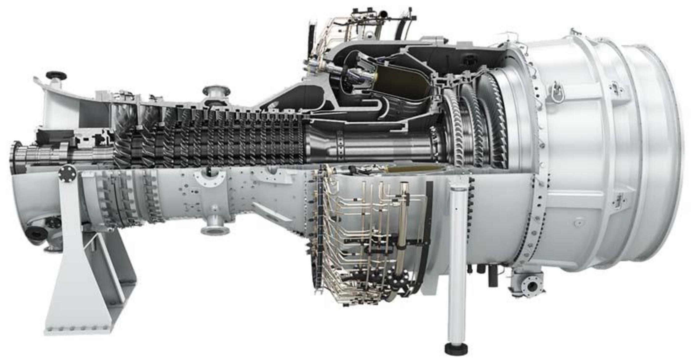
2. Description of Gas Turbine and its Start-Up Process

The SGT 600, an industrial gas turbine of medium size with two shafts is investigated in this article. This setup can be utilized in mechanical-drive and power generation applications [38]. Known as one of the most reliable gas turbine in its power range, the SGT 600 comprises an axial compressor that possesses 10 stages, of which the first two include variable inlet guide vanes. To prevent surging, the studied engine benefits from two bleed valves that can open at start to guarantee the stability and integrity for the engine. Table 1 lists the engine properties at design point [38]. In addition, the examined gas turbine includes two specific components: (1) gas generator (referred to as GG), and (2) power turbine (referred to as PT). The former supplies the energy required for the rotary motion of the latter, which in turn is used to rotate the compressor or generator based on relevant applications. The offset section view of the SGT 600 and is shown in Figure 5.
The variation of performance parameters of the turbine during cold start-up phase is as follow: the rpm of GG shaft is first increased using the electric starter until it hits a certain amount (cranking). It spends some time at this rpm (purging), followed by sparking and combustion.
As can be seen in Figure 6, after starting, the clutch is engaged and the starter increases GG speed up to 2300 rpm. The starter remains at the same speed from this point and the clutch is in D state. However, due to the rotor inertia force, NGG slightly increases (it experiences a jump) and then returns to 2300 rpm once more such that the clutch is put in E state. The starter and GG rotate with each other for 75 s until the gas turbine is purged (freeing any left gas). After 75 s, the clutch reaches D state so that the flame can be created, preventing it from being put out by air speed. Once NGG reaches 1620 rpm, the flame is created and the clutch turns into E state again. From this moment on, the starter and CC (combustion chamber) cooperatively increase NGG. Once the speed get to the self-sustaining stage, the clutch will be in D state, after which CC increases NGG up to working rpm. After the operation of gas turbine for the desired amount of time, the shutdown command arrives at the motor and the starter is turned on (200 rpm). GG rpm decreases after shutting down until it hits 200 rpm.

3. Bond Graph Modeling of Components During Cold Start

To launch the industrial gas turbine with the aid of an electric starter motor, control of the induction motor using SFC is necessary since the turbine inertia is high and in cases where the motor tends to rotate such loads with direct connection to the distribution network, the starting current of motor would be too high, causing severe thermal and mechanical damages to the motor. Moreover, sudden start of motor exerts stress to the turbine shaft and other mechanical parts. Figure 7 shows the general diagram of the simulated system. After starting the induction motor using the drive, power transmission to the turbine shaft is controlled via the automatic clutch mechanism.
A comprehensive study by Åström et al. on evolution of continuous-time modeling and simulation shows that there are several problems in complicated/mechatronic systems modeling when analog and numerical simulation tools are used [39]. Astrom et al. confirms this issues by some examples in [39]. They showed that even for simple system (a motor drive with an electric motor, a gearbox, a load, and a controller), if the detailed equations are considered to implement directly there will be a loop which only contains algebraic equations. The phenomenon which is well known in analog simulation is called the algebraic loop problem. One way of dealing with it in analog computing was to introduce a small capacitor in the algebraic loop. With respect to these conclusions, physical modeling approaches are suggested for integrated modeling and simulations. Especially, for mechatronic systems, bond graphs is a very high potential candidates. Bond graphs are directed graphs where the subsystems are the nodes and the power flow in the system is shown by the branches. The connections are called power bonds and have associated effort variables (such as voltage and torque) and flow variables (current and angular velocity). This approach is used successfully by the authors in the field of gas turbine engines modeling and simulation and the effectiveness is confirmed against theoretical and experimental data [40,41,42].

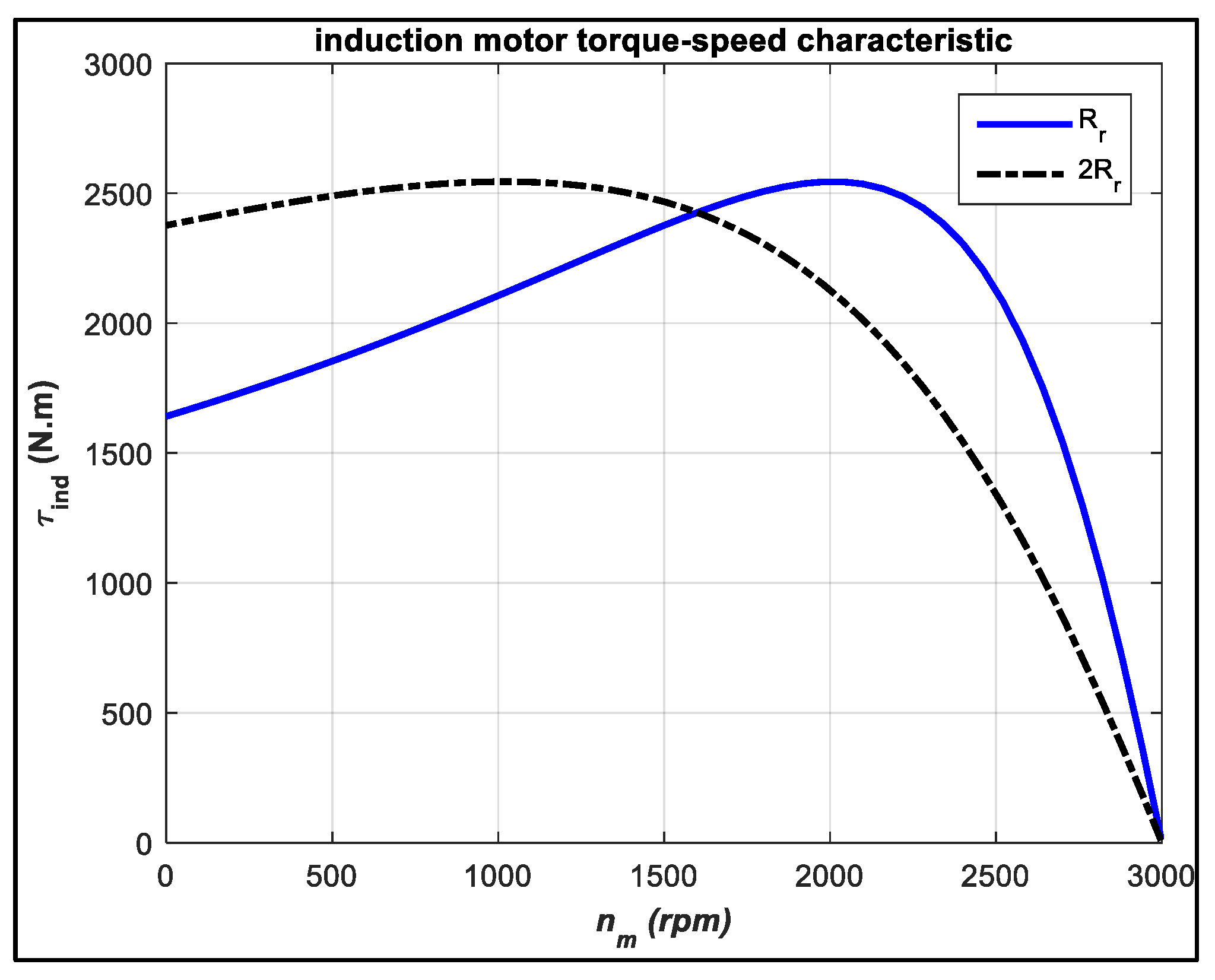
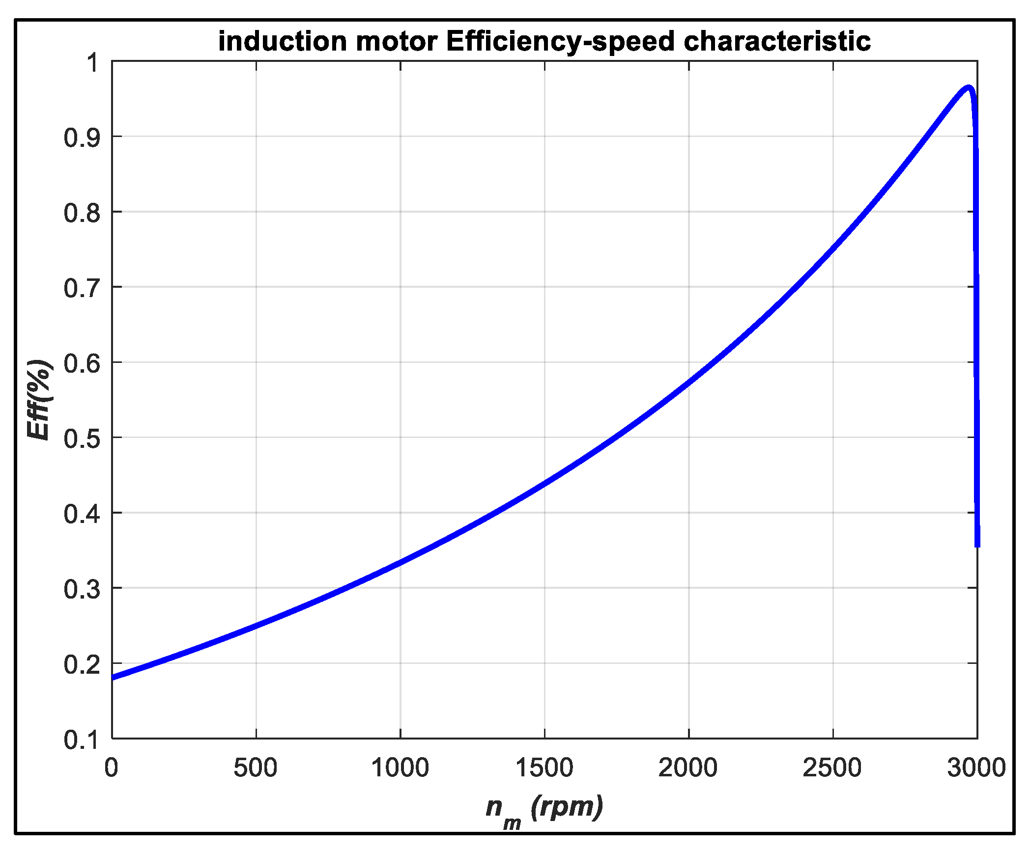
3.1. Modeling the Induction Motor and SFC Drive

Thermal, electrical, and mechanical stresses may constantly be exerted on electric drive systems. As a result, one needs to take great care of simulation and modeling of such devices so as to be able to properly examine their behavior. What might cause some technical issues is that electric starters are modeled independently to the rest of the subsystems in simulation environments. Coupling the models developed for each subsystems and the occurrence of numerical problems such as algebraic loop in simulation are among this group [39]. When simulating a hybrid system composed of electric starter and gas turbine, we are dealing with algebraic and differential governing equations of the system. An algebraic loop constantly occurs when these equations are implemented in the conventional software (including Matlab) as a means of simulation. This is one of the challenges of simulation and modeling of mechatronic systems including the above system. Modern tools like Modelica, Simscape with Simpower, Simdriveline (which is Mathworks incarnation of Modelica), and bond graph can effectively tackle this issue. Another innovation of the present article is that modeling the electric starter is achieved through bond graph methodology and is then linked to the model of gas turbine.
The induction motor is a type of alternative current motor, i.e., an asynchronous AC motor whose necessary power in its moving part is provided using electromagnetic induction. AC induction motors are the most common types of motors used in industrial gas turbines. Since exact data concerning the induction motor of SGT600 gas turbine is not accessible, the start-up process plot of Ref. [21] is instead used. According to this plot, it can be concluded that the maximum nominal speed of induction motor is equal to 3000 rpm. Moreover, the required torque for the turbine to reach the purging stage is found from Ref. [43]. Considering these two values, the nominal power of the induction motor is obtained. Moreover, the supply voltage is taken from the power network. In the following, modeling the induction motor and SFC drive is studied.

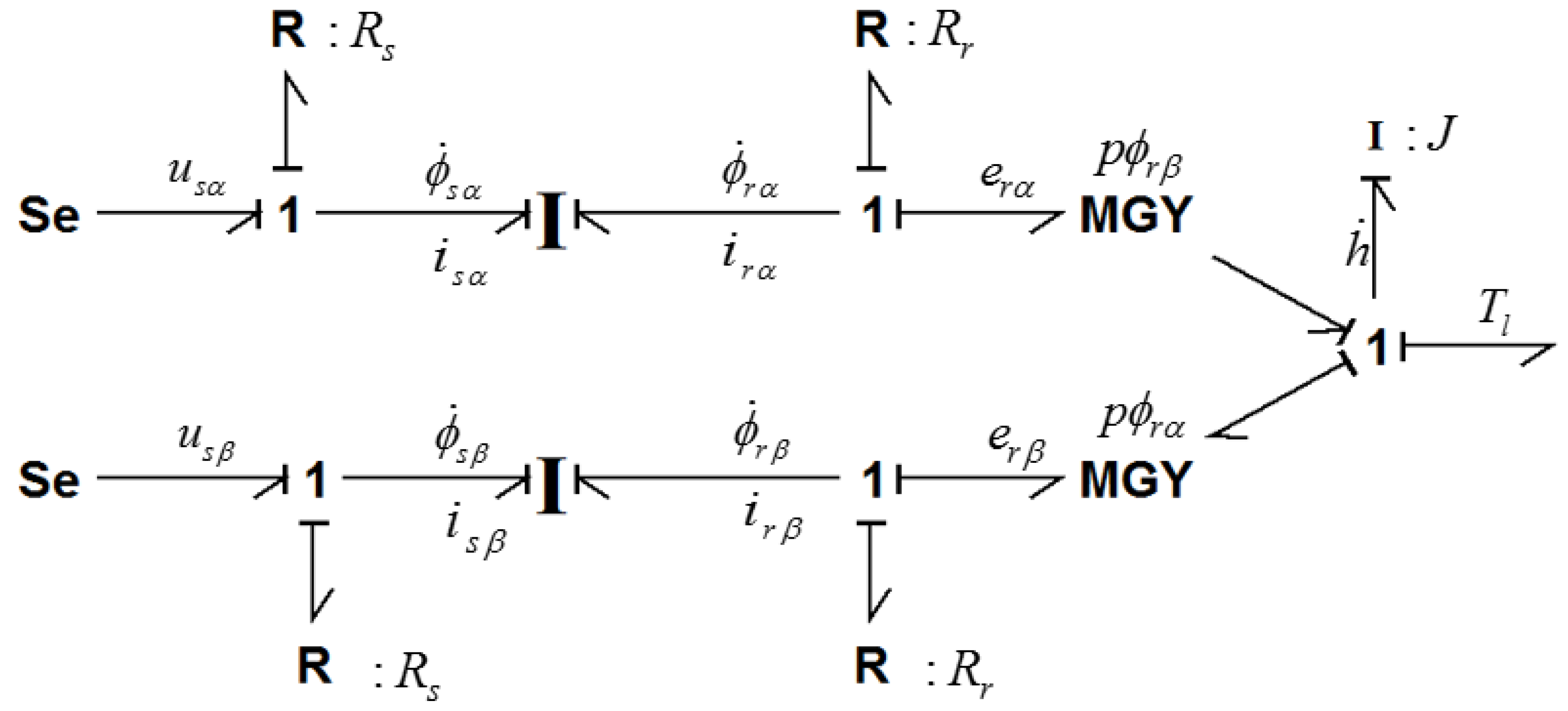
3.1.1. Modeling the Induction Motor Using Bond Graph

Circuit form representation of induction motors regarding their steady state characteristics at constant speed, especially under sinusoidal excitation, has been a common trend, providing the ability to obtain the valuable plots of torque versus speed [44]. However, complicated control strategies on current or voltage should be implemented when dealing with variable speed drives. Such control techniques are mainly designed with respect to the motor’s dynamic model. For the general theory on electrical machines with rotary motion, the reader is referred to Refs. [45,46,47], which present the standard model of an induction motor. It should be noted that certain recent studies tend to demonstrate the model of induction motors as nonlinear state equations (of fifth order) or alternatively, using an analogous circuit, although the mechanical components are not visible [45]. In the following, the presented model equations are similar to those of some other researches [48,49,50] where the two-phase model belonging to the motor is described in a reference frame of α β , fixed and located on the stator. The notations and main parameters of such models vary by author, and different variables are taken as state variables, while the reasons behind the selection of state variables are usually left unexplained and different combined parameters are exploited, leading to different representation. Here, the notations of Karnopp [51] are mainly utilized:
d i s α d t = μ i s α + M R r σ L s L r 2 ϕ r α + p M σ L s L r ω ϕ r β + u s , α σ L s ,
d i s β d t = μ i s β + M R r σ L s L r 2 ϕ r β p M σ L s L r ω ϕ r α + u s , β σ L s ,
d ϕ r α d t = R r L r ϕ r α p ω ϕ r β + M R r L r i s α ,
d ϕ r β d t = p ω ϕ r α R r L r ϕ r β + M R r L r i s β ,
d ω d t = k T J ( ϕ r α i s β ϕ r β i s α ) T l J .
where R r and R s are the resistances of rotor and stator, L r and L s are the corresponding self-inductances, M represents the common mutual inductance, J depicts the moment of inertia and T l is the load torque. It should be noted that the process of obtaining two-phase variables from three-phase variables is not explained here for the sake of brevity. In addition, certain assumptions are made, including the linearity of magnetic circuits, while the control inputs are ( u s , α , u s , β ) (voltages of stator) and the state variables are takes as follows: ω (mechanical speed of rotor), ( ϕ r α , ϕ r β ) (fluxes of rotor), and ( i s α , i s β ) (currents of stator). Finally, p is the number of pole pairs and k T = p M / L r displays the joined parameters. Moreover,
μ = R s / σ L s + R r M 2 / σ L s L r 2 , σ = 1 M 2 / L s L r
When the stator currents are assumed to come from sources with stiff current, and are used at control inputs of the motor, then Equations (3)–(5) represent the third-order motor model, neglecting Equations (1) and (2) altogether.

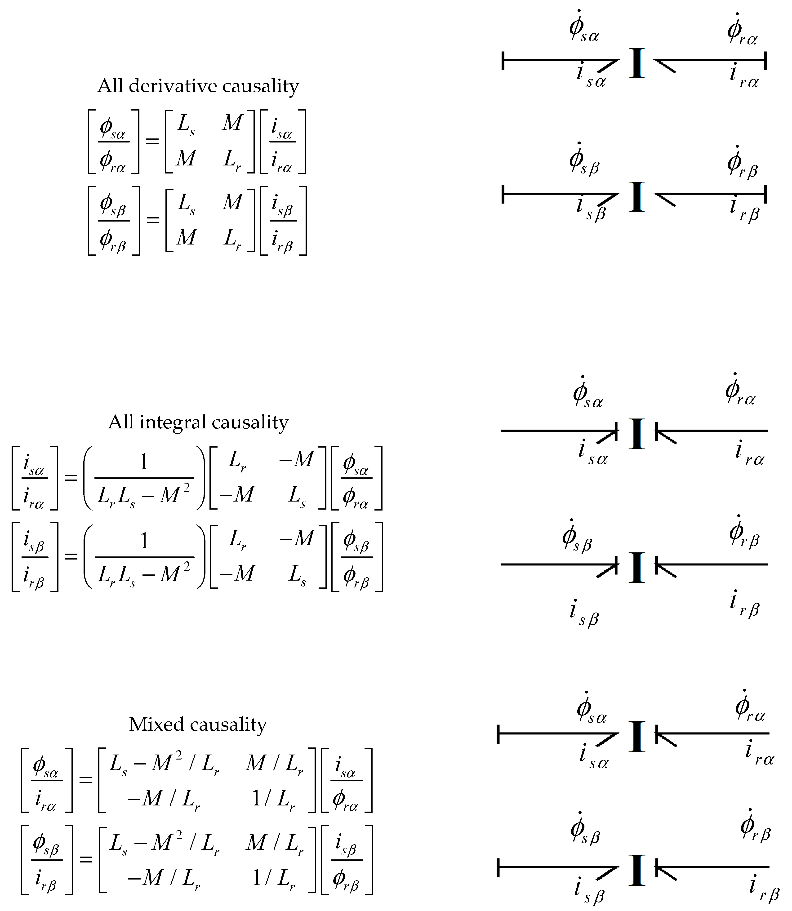
Inductive Coupling of Rotor and Stator

The inductive coupling existing between rotor and stator described in α and β axes is considered foremost. The parameters of mutual and self inductances are utilized to show the relationship between currents and fluxes. These linear relationships are simply displayed using I-fields in the bond graph approach, as depicted in Figure 8 where these I-fields in different forms along with related matrix equations can be seen. The derivative causality can be considered as the most basic equation on each I-field bond. Logically, the all-integral version for such I-field equations is employed in a bond graph model and the mixed-causality one is suitable when control inputs are assumed to be stator currents. The reason why certain combined parameters including σ occur, can be traced back to the inversion process of induction matrix and L s L r M 2 as the accompanying factor.

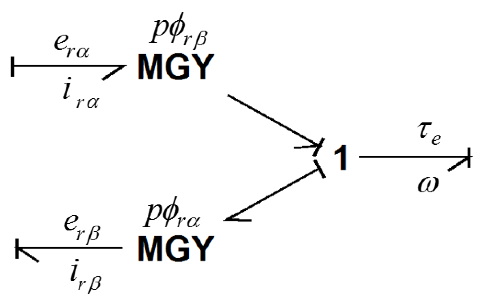
Representation of Torque and Induced Voltage in Bond Graph

The previously-mentioned model equations contain certain complexities, in part due to the choice of state variables. First, the induced voltage might seem to be commensurate to the mechanical speed, whereas the coefficients are actually different since the currents and fluxes are selected for the stator and rotor, respectively. Second, the power conservation related to different mechanical and electrical variables is not easily recognized as a combination of current and flux terms are used in the torque equation. The corresponding bond graph model of gyrator, nevertheless, provides a clear means of obtaining a gyrator structure used for the induction motor. The concurrent relation between the speed and induced voltage along with the relation between currents and fluxes to the torque is displayed in Figure 9.
One can easily observe the voltage terms that appeared in Equations (3) and (4) in Figure 10, as in
e r α = p ϕ r β ω , e r β = p ϕ r α ω .
while this is not exactly true for the generated torque. After some manipulation and using the mixed causality depicted in Figure 9, an appropriate relation for the torque from the bond graph is obtained as
τ e = ( p M / L r ) ( ϕ r α i s β ϕ r β i s α ) = p ( ϕ r β i r α ϕ r α i r β )
Through the use of bond graph, one can verify the power conserving nature of the conversion of electromechanical energy.

Bond Graph for the Induction Motor

The set of equations presented in this section can be represented using Figure 10. However, the bond graph model utilized four fluxes instead of two currents and two fluxes and as a result, the associated equation of the displayed causality may seem different. In addition, the angular velocity ω has been replaced by the angular momentum h in the bond graph.
The advantage of bond graph is that there is no need to explicitly list the equations when a processor for the bond graph is available. It should also be noted that the integral causality is preferred for the representation of I-field. As a comparison, one can obtain the new set of equations in the form
ϕ ˙ s α = R s L r ( L r L s M 2 ) ϕ s α + R s M ( L r L s M 2 ) ϕ r α + u s α
ϕ ˙ s β = R s L r ( L r L s M 2 ) ϕ s β + R s M ( L r L s M 2 ) ϕ r β + u s β
ϕ ˙ r α = R r L s ( L r L s M 2 ) ϕ r α + R r M ( L r L s M 2 ) ϕ s α p ϕ r β h J
ϕ ˙ r β = R r L s ( L r L s M 2 ) ϕ r β + R r M ( L r L s M 2 ) ϕ s β + p ϕ r α h J
h ˙ = p ϕ r β ( L s ϕ r α M ϕ s α ) ( L r L s M 2 ) p ϕ r α ( L s ϕ r β M ϕ s β ) ( L r L s M 2 ) T L
which seem more complicated than Equations (1)–(5). The introduction of some ancillary parameters may simplify this issue. In the case the current sources drive the motor model instead of voltage sources, the number of state variables dictated by causality is only three. This implies that except using h instead of ω , the consequent equations would be similar to Equations (2)–(5) and the mixed causality previously displayed in Figure 9 is a suitable option.

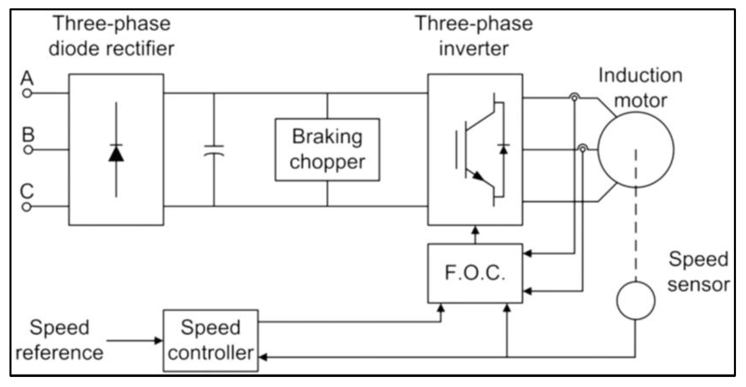
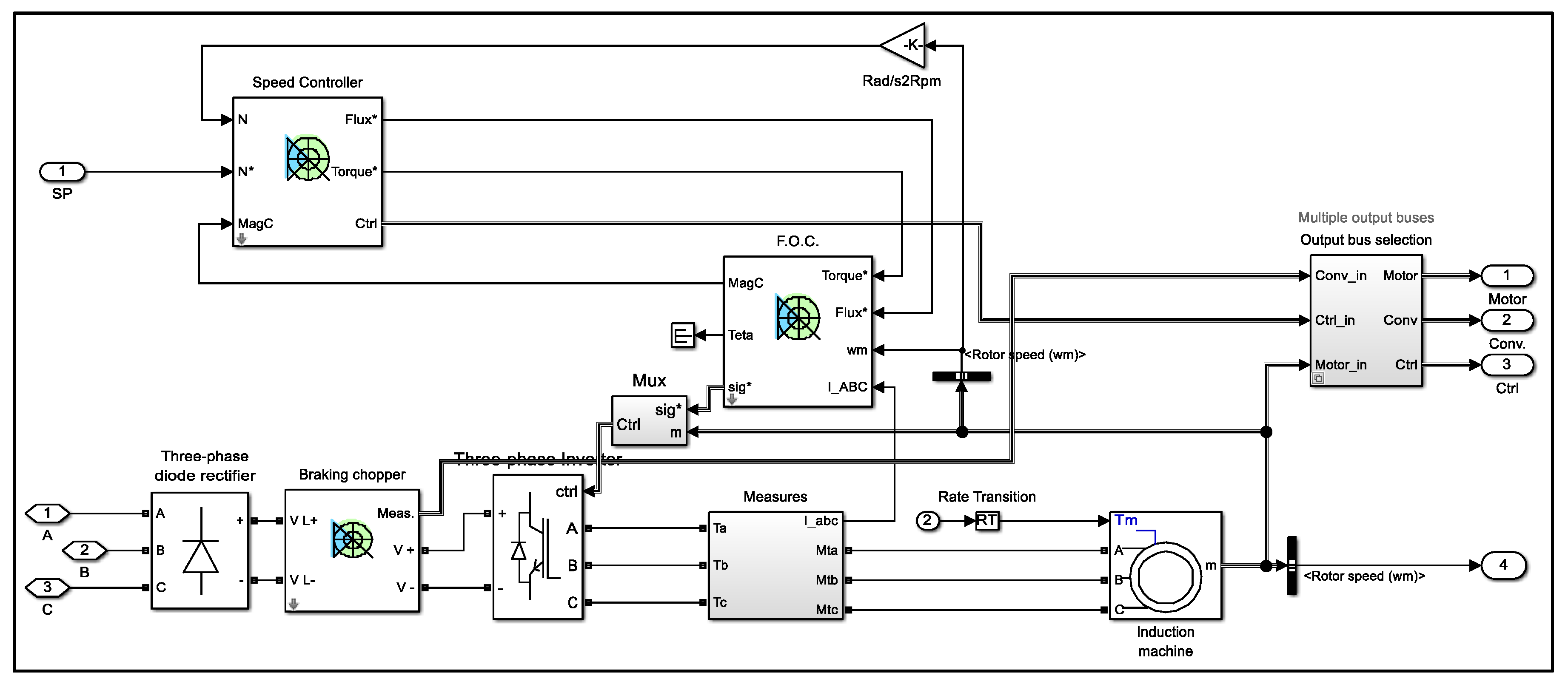
3.1.2. Modeling SFC Drive

The main components of the drive include three-phase diode rectifier for generation of desired AC voltage, DC link, DC link chopper, three-phase inverter for generation of AC voltage with suitable amplitude and frequency for supplying the induction motor, and breaking chopper for controlling the DC link with capacitor energy difference in resistance when the acceleration is negative or the loading torque accelerates the motor. Speed sensors and controller, along with current sensor and drive controller system are based on the field oriented control (F.O.C). SFC drive structure is shown in Figure 11. The designed drive that is connected to three-phase electrical grid with an effective voltage of 400 V and frequency of 50 Hz controls the induction motor. Figure 12 displays the internal structure of the drive used in simulation which was designed in Matlab/Simulink.

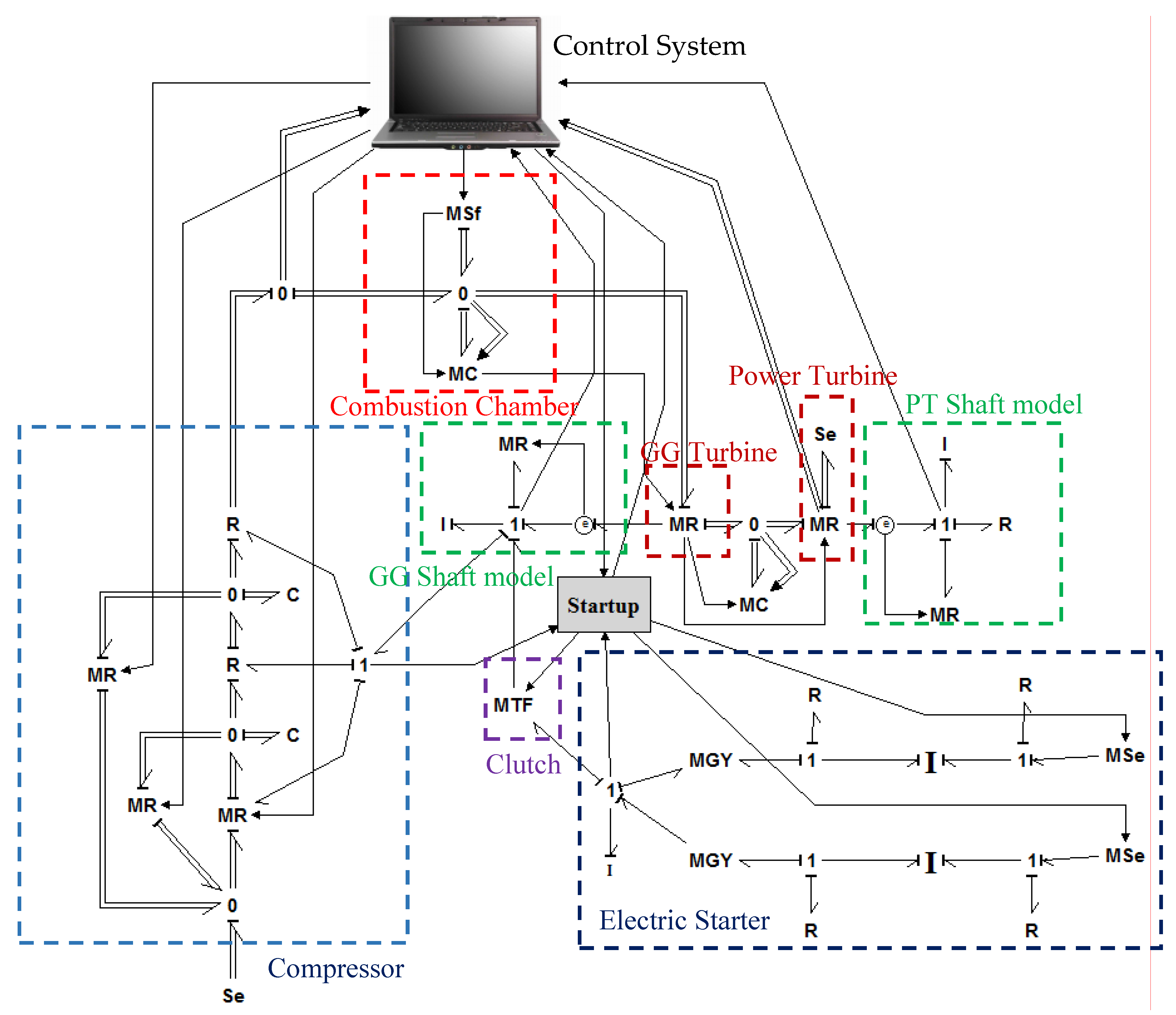
3.2. Modeling the Industrial Gas Turbine

The bond graph model of gas turbine used in this study is developed and described by the authors of this study in Refs. [38,52,53]. For a better understanding of gas turbine modeling procedure using bond graph, the reader is encouraged to read the mentioned references. Figure 13 is a description of the gas turbine bond graph model.

4. Completed Model of Gas Turbine in Cold Start-Up Phase

By combining the bond graph models developed in previous sections, the completed bond graph model of the mentioned mechatronic system is obtained according to Figure 13. A section named “start-up” is observed in this figure. SFC drive and clutch controller are located in this section. The goal of this section is to control the induction motor and clutch during start-up. This section is connected to the gas turbine control system through two information bonds. One bond sends the information to the turbine control system and the other bond receives the information from that. Two other information bonds are sent to voltage sources through SFC drive and modulates them. The clutch along with a modulated transformer (MTF) is shown in Figure 14. Controlling the clutch is realized via information exchange with start-up section. The speed of input shaft connected to the electric starter is sent to the start-up section from 1-juction in the induction motor model via an information bond. The output shaft speed connected to the gas turbine compressor is sent to the start-up section from 1-juction in turbine model via another information bond. By comparing the input and output shaft speeds in the start-up section, a decision concerning the engagement or engagement of clutch in this section is made. This decision is sent to the clutch from another information bond and modulate it. For instance, immediately after the input speed is reduced with respect to the output speed, the clutch is disengaged.

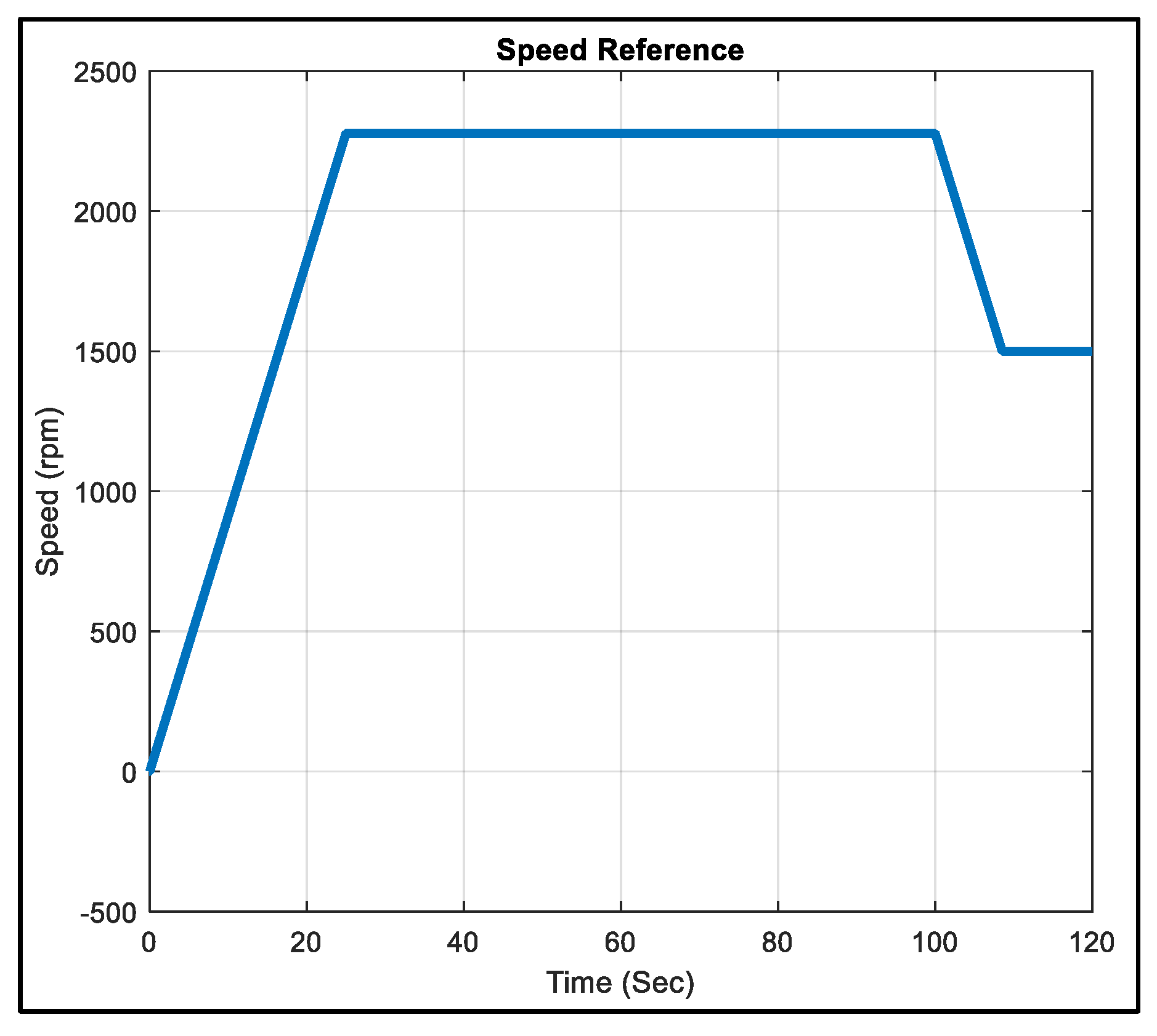
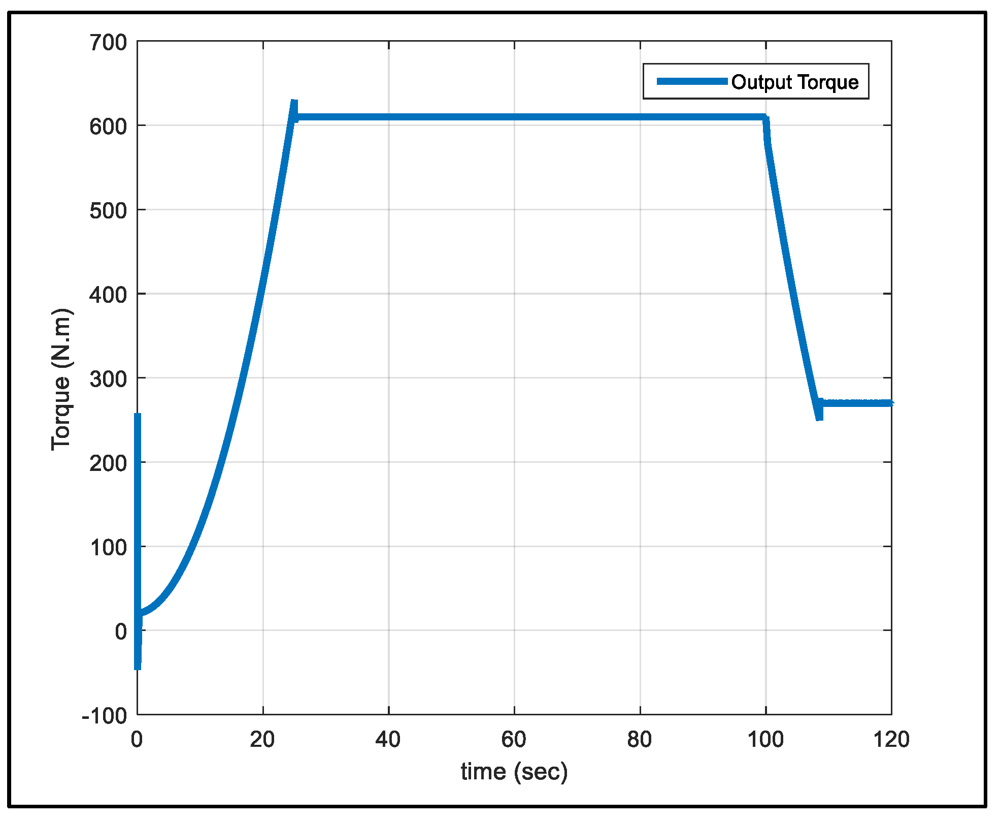
5. Analysis of Simulation Results

The specifications of the studied induction motor are presented in Table 2. According to this table, the parameters of the induction motor are listed in Table 3. Moreover, Table 4 shows the simulation parameters.
The characteristic torque-speed of the induction motor under study with two different rotor resistances is shown as in Figure 14. As the rotor resistance increases, the starting torque and the sliding amount at which the maximum torque occurs change.
As obvious in Figure 14, the increase in the rotor resistance also increases the starting torque, while reducing the speed at which the maximum torque occurs. Figure 15 shows the variations of induction motor efficiency with respect to speed. As can be noticed, the highest efficiency of the machine happens to be around the synchronous speed.
Noting the pre-described conditions for the induction motor motion, the speed reference in this section is built upon the empirical test curve as well as the reference curve [21]. Figure 16 shows the utilized speed reference.
According to Figure 16, the speed reference has four parts. In the first part, the speed increases with constant acceleration and reaches 2278 rpm at t = 25 s. Then, it remains constant for 75 s, after which the motor speed decreases for around 8.5 s and reaches the constant velocity of 1500 rpm at which it continues its operation. Table 5 shows the properties of the used drive.
In this section, based on the speed reference curve, the set of network–drive–starter motor–gas turbine is simulated. Figure 17 shows the torque–time plot of turbine output.
The amount of above-mentioned effective current is obtained as
I r m s = 1 T T i 2 ( t ) d t
Figure 18 shows the extracted current–time from the network by motor–drive set and Figure 19 shows the details of extracted current from the network by the motor–drive set and stator current.
As can be seen in Figure 18 and Figure 19, the extracted current form the network is intensely harmonic which is natural in existence of drive as a nonlinear load. By altering the amplitude and frequency of the motor terminal voltage, motor control drives are able to control the output speed or torque of the motor based on speed reference or torques. As a result, the extracted current from the network is highly harmonic. Figure 20 shows THD (Total Harmonic Distortion), a measurement of the harmonic distortion present in a signal and is defined as the ratio of the sum of the powers of all harmonic components to the power of the fundamental frequency, of extracted current from the network. THD value is obtained as:
T H D I = k = 2 I k 2 I 1
where I 1 is the main component of current and I k is the kth harmonic component of current.
In Figure 20, the very high value of THD during initial moments is due to measurement error caused by the generated transients at drive starting moment. After the initial transients, it is observed that THD value is reduced after some time and accompanied by the increase in motor speed and torque. When the speed, output torque and, consequently, output power of motor in addition to the input power of drive become constant, THD value also remains the same. At t = 100 s and with the decrease in speed along with changes in torque and power, THD value rises. DC bus voltage is displayed in Figure 21.
According to Figure 21, the average DC bus voltage decreases during motor acceleration, and remains constant when the motor output speed and torque are held constant as the power does not change. Variations of DC bus voltage occurs due to the switching of power electronic switches used in the inverter. Figure 22 shows the calculated output mechanical power from P = T ω as a function of time along with the input electric power.
As visible in Figure 22, during the time interval of t = 0–25 s, when the load required mechanical power is increasing, the input electric power to the motor – drive set also increases. In fact, the drive input power is equal to the sum of load required mechanical power and electric and mechanical dissipations of motor–drive set.
Figure 23, shows the total active (P) and reactive (Q) power extracted from the network. Furthermore, Equation (16) describes the relation used for obtaining the total active and reactive power extracted from the network in which I L and V L L are, respectively, the effective current and effective voltage of the electrical grid.
P = 3 V L L I L cos φ Q = 3 V L L I L sin φ
Figure 24 shows the active and reactive power of the main three-phase frequency extracted from the network. The amount of active and reactive power of the main frequency extracted from the network is found using Equation (17) in which I L 1 and V L L 1 are, respectively, the effective current and effective voltage of the main component of network line and φ 1 is the phase difference between the two.
P = 3 V L L 1 I L 1 cos φ 1 Q = 3 V L L 1 I L 1 sin φ 1
As noticeable by analyzing the two figures above, the little difference between the total active power and the active power of the main component is due to the fact that the harmonic constituent of the input voltage of drive is too low and, therefore, the active power consumed by harmonic components is negligible. Due to the harmonic nature of the current extracted from the drive, as shown in Figure 19, the total distortion reactive power and the main component reactive power are noticeable and these two reactive powers display a dramatic difference such that the reactive power of main component is positive, while the total reactive power is negative. This large difference occurs because the main portion of the power generated from harmonic components are of the reactive type. Figure 25 shows the variation of the induction motor input frequency during studying period.
As evident from Figure 25, the motor input frequency increases according to the speed reference curve. When the speed is constant around 2400 rpm, the motor input frequency is held constant by the drive at 80 Hz. Figure 26 displays the induction motor input voltage.
As can be seen in Figure 26, at times when an increase in speed is required based on the speed reference curve, the input voltage is also increased by the drive.

6. Conclusions

Gas turbine utilization in the power industry has seen an increasing trend in recent years. By properly optimizing the gas turbine performance during start-up, emergency power demand on the electrical grid can be better responded. Starting is still one of the most important challenges when designing and operating gas turbines across the world. Accordingly, modeling the cold start-up phase of industrial gas turbine is studied in this article. During this phase, an asynchronous AC motor controlled by a SFC drive exists as electric starter. Bond graph models of these components are developed in this study. Vector control systems represented by their dynamic equations and used for controlling the speed of induction motor drives can be appropriately represented through the use of bond graph. Modeling complete systems is thus possible as the mechanical port exists explicitly. Finally, the bond graph model of asynchronous motor is coupled to the gas turbine model through the mechanical port. Start-up speed reference is selected according to empirical tests such that the technical requirements imposed on the gas turbine are satisfied. Simulation results can prove the proper performance of the system during start-up.

Author Contributions

Methodology, S.A.M.F.; Supervision, T.N.; Writing—review & editing, S.J.

Funding

This research received no external funding.

Conflicts of Interest

The authors declare no conflict of interest.

References and Note

  1. Siemens AG. Modernizations and Upgrades—Siemens. 2018. Available online: https://www.energy.siemens.com/hq/en/services/fossil-power-generation/modernization-upgrades/ (accessed on 10 February 2018).
  2. General Electric. Aeroderivative & Heavy-Duty Gas Turbines|GE Power. 2018. Available online: https://www.gepower.com/gas/gas-turbines (accessed on 20 January 2018).
  3. ALSTOM. Alstom’s World Class Gas Turbine Technology Enters Commercial Operation in China. 2014. Available online: http://www.alstom.com/press-centre/2014/3/alstoms-world-class-gas-turbine-technology-enters-commercial-operation-in-china-/ (accessed on 8 December 2017).
  4. Balling, L. Fast cycling and rapid start-up: New generation of plants achieves impressive results. Mod. Power Syst. 2011, 31, 35–41. [Google Scholar]
  5. Western Turbine Users. LM6000 Product Breakout Session; General Electric Company: Long Beach, CA, USA, 2015. [Google Scholar]
  6. Poluéktova, E. Results of Model Studies of the Control System of a Gas-Turbine Unit with a Free Power Turbine. Power Technol. Eng. 2017, 51, 459–463. [Google Scholar] [CrossRef]
  7. Bahlawan, H.; Morini, M.; Pinelli, M.; Spina, P.R.; Venturini, M. Development of Reliable NARX Models of Gas Turbine Cold, Warm and Hot Start-Up. In Proceedings of the ASME Turbo Expo 2017: Turbomachinery Technical Conference and Exposition, Charlotte, NC, USA, 26–30 June 2017; p. V009T027A007. [Google Scholar]
  8. Asgari, H.; Venturini, M.; Chen, X.; Sainudiin, R. Modeling and simulation of the transient behavior of an industrial power plant gas turbine. J. Eng. Gas Turbines Power 2014, 136, 061601. [Google Scholar] [CrossRef]
  9. Morini, M.; Cataldi, G.; Pinelli, M.; Venturini, M. A Model for the Simulation of Large-Size Single-Shaft Gas Turbine Start-Up Based on Operating Data Fitting. In Proceedings of the ASME Turbo Expo 2007: Power for Land, Sea, and Air, Montreal, QC, Canada, 14–17 May 2007; pp. 1849–1856. [Google Scholar]
  10. Zhang, Y.; Cruz-Manzo, S.; Latimer, A. Start-up vibration analysis for novelty detection on industrial gas turbines. In Proceedings of the International Symposium on 2016 Industrial Electronics (INDEL), Santa Clara, CA, USA, 8–10 June 2016; pp. 1–6. [Google Scholar]
  11. Mahdipour, M.; Bathaee, S.M.T. A novel static frequency converter for start-up and shutdown processes of gas turbine power plant units. Int. Trans. Electr. Energy Syst. 2015, 25, 3586–3599. [Google Scholar] [CrossRef]
  12. An, H.; Han, B.-M.; Cha, H. A new sensorless start-up method of LCI system for gas-turbine. In Proceedings of the 2015 IEEE Energy Conversion Congress and Exposition (ECCE), Montreal, QC, Canada, 20–24 September 2015; pp. 6559–6564. [Google Scholar]
  13. An, H.; Cha, H. A New Start-up Method for a Load Commutated Inverter for Large Synchronous Generator of Gas-Turbine. J. Electr. Eng. Technol. 2018, 13, 201–210. [Google Scholar]
  14. Bretschneider, S.; Reed, J. Modeling of Start-Up from Engine-Off Conditions Using High Fidelity Turbofan Engine Simulations. J. Eng. Turbines Power 2016, 138, 051201. [Google Scholar] [CrossRef]
  15. Sheng, H.; Zhang, T.; Jiang, W. Full-Range Mathematical Modeling of Turboshaft Engine in Aerospace. Int. J. Turbo Jet-Engines 2016, 33, 309–317. [Google Scholar] [CrossRef]
  16. Sukhovii, S.I.; Sirenko, F.F.; Yepifanov, S.V.; Loboda, I. Alternative method to simulate a Sub-idle engine operation in order to synthesize its control system. Int. J. Turbo Jet-Engines 2016, 33, 229–237. [Google Scholar] [CrossRef]
  17. Cao, Y.; Wang, J.; Dai, Y.; Xie, D. Study of the speed control system of a heavy-duty gas turbine. In Proceedings of the ASME Turbo Expo 2015: Turbine Technical Conference and Exposition, Montreal, QC, Canada, 15–19 June 2015; p. V006T005A014. [Google Scholar]
  18. Hu, Z.; Jiang, B.; Wang, J.; He, X. A generalized method for sub-idle modeling of aircraft engines. In Proceedings of the 2017 8th International Conference on Mechanical and Aerospace Engineering (ICMAE), Prague, Czech Republic, 22–25 July 2017; pp. 527–531. [Google Scholar]
  19. Agrawal, R.; Yunis, M. A generalized mathematical model to estimate gas turbine starting characteristics. J. Eng. Power 1982, 104, 194–201. [Google Scholar] [CrossRef]
  20. Kim, J.; Song, T.; Kim, T.; Moverare, J. Dynamic simulation of full start-up procedure of heavy duty gas turbines. In Proceedings of the ASME Turbo Expo 2001: Power for Land, Sea, and Air, New Orleans, LA, USA, 4–7 June 2001; p. V004T004A010. [Google Scholar]
  21. Blomstedt, M.; Lindgren, H.; Olausson, H.-L.; Moverare, J. Innovative starting procedure of Siemens SGT-600 in cold climate conditions. In Proceedings of the ASME 2011 Turbo Expo: Turbine Technical Conference and Exposition, Vancouver, BC, Canada, 6–10 June 2011; pp. 1021–1026. [Google Scholar]
  22. Montazeri-Gh, M.; Miran, F.S.A. Application of bond-graph method in microjet engine cold start modeling to investigate the idea of injecting compressed air. Appl. Mech. Mater. 2015, 799–800, 890–894. [Google Scholar] [CrossRef]
  23. Miran, F.S.A.; Montazeri-Gh, M. Modeling and Simulation of JetQuad Aerial Robot Knowledge-Based Engineering and Innovation (KBEI); Iran University of Science and Technology (IUST): Tehran, Iran, 2017. [Google Scholar]
  24. Asgari, H.; Chen, X.; Morini, M.; Pinelli, M.; Sainudiin, R.; Spina, P.R.; Venturini, M. NARX models for simulation of the start-up operation of a single-shaft gas turbine. Appl. Therm. Eng. 2016, 93, 368–376. [Google Scholar] [CrossRef]
  25. Nannarone, A.; Klein, S.A. Start-Up Optimization of a CCGT Power Station Using Model-Based Gas Turbine Control. J. Eng. Gas Turbines Power 2019, 141, 041018. [Google Scholar] [CrossRef]
  26. Yoshida, Y.; Yoshida, T.; Enomoto, Y.; Osaki, N.; Nagahama, Y.; Tsuge, Y. Start-up optimization of combined cycle power plants: A field test in a commercial power plant. J. Eng. Gas Turbines Power 2019, 141, 031002. [Google Scholar] [CrossRef]
  27. Tsoutsanis, E.; Meskin, N. Dynamic performance simulation and control of gas turbines used for hybrid gas/wind energy applications. Appl. Therm. Eng. 2019, 147, 122–142. [Google Scholar] [CrossRef]
  28. Borutzky, W. Bond graph modelling and simulation of multidisciplinary systems an introduction. Simul. Model. Pract. Theory 2009, 17, 3–21. [Google Scholar] [CrossRef]
  29. Karnopp, D.C.; Margolis, D.L.; Rosenberg, R.C. System Dynamics: Modeling, Simulation, and Control of Mechatronic Systems; John Wiley & Sons: Hoboken, NJ, USA, 2012. [Google Scholar]
  30. Brown, F.T. Engineering System Dynamics: A Unified Graph-Centered Approach; CRC Press: Boca Raton, FL, USA, 2006. [Google Scholar]
  31. Uddin, N.; Gravdahl, J.T. Bond graph modeling of centrifugal compression systems. Simulation 2015, 91, 998–1013. [Google Scholar] [CrossRef]
  32. Munari, E.; Morini, M.; Pinelli, M.; Brun, K.; Simons, S.; Kurz, R. Measurement and Prediction of Centrifugal Compressor Axial Forces During Surge—Part II: Dynamic Surge Model. J. Eng. Gas Turbines Power 2018, 140, 012602. [Google Scholar] [CrossRef]
  33. Munari, E.; Morini, M.; Pinelli, M.; Spin, P.R. Experimental Investigation and Modeling of Surge in a Multistage Compressor. Energy Procedia 2017, 105, 1751–1756. [Google Scholar] [CrossRef]
  34. Sanei, A.; Novinzadeh, A.; Habibi, M. Addition of momentum and kinetic energy effects in supersonic compressible flow using pseudo bond graph approach. Math. Comput. Model. Dyn. Syst. 2014, 20, 491–503. [Google Scholar] [CrossRef]
  35. Yum, K.K.; Pedersen, E. Architecture of model libraries for modelling turbocharged diesel engines. Math. Comput. Model. Dyn. Syst. 2016, 22, 584–612. [Google Scholar] [CrossRef]
  36. Movaghar, A.S.; Novinzadeh, A. Ideal Turbo charger Modeling and Simulation using Bond Graph Approach. In Proceedings of the ASME 2011 Turbo Expo: Turbine Technical Conference and Exposition: American Society of Mechanical Engineers, Vancouver, BC, Canada, 6–10 June 2011; pp. 871–879. [Google Scholar]
  37. Vangheluwe, H.; de Lara, J.; Mosterman, P.J. An introduction to multi-paradigm modelling and simulation. In Proceedings of the AIS2002 Conference (AI, Simulation and Planning in High Autonomy Systems), Lisboa, Portugal, 7–10 April 2002; pp. 9–20. [Google Scholar]
  38. Montazeri-Gh, M.; Fashandi, S.A.M. Application of Bond Graph approach in dynamic modelling of industrial gas turbine. Mech. Ind. 2017, 18, 410. [Google Scholar] [CrossRef]
  39. Åström, K.J.; Hilding, E.; Dynasim, A.; Sven, E.M. Evolution of Continuous-Time Modeling and Simulation. In Proceedings of the 12th European Simulation Multiconference, Manchester, UK, 16–19 June 1998. [Google Scholar]
  40. Montazeri-Gh, M.; Miran Fashandi, S.A.; Jafari, S. Theoretical and Experimental Study of a Micro Jet Engine Start-Up Behaviour. Tech. Gaz. 2018, 25, 839–845. [Google Scholar]
  41. Montazeri-Gh, M.; Miran Fashandi, S.A.; Abyaneh, S. Real-time simulation test-bed for an industrial gas turbine engine’s controller. Mech. Ind. 2018, 19, 311. [Google Scholar] [CrossRef]
  42. Jafari, S.; Miran Fashandi, S.A.; Nikolaidis, T. Control Requirements for Future Gas Turbine-Powered Unmanned Drones: JetQuads. Appl. Sci. 2018, 8, 2675. [Google Scholar] [CrossRef]
  43. Nordström, L. Construction of a Simulator for the Siemens Gas Turbine SGT-600; Institutionen för Systemteknik: Linköping, Sweden, 2005. [Google Scholar]
  44. EMI Induction Motor Data Sheet, Motor Type: EM1-315L2-2 200KW 400 690V 50HZ.
  45. Bose, B.K. Modern Power Electronics and AC Drives; Prentice Hall PTR: Upper Saddle River, NJ, USA, 2002. [Google Scholar]
  46. Krause, P.C. Analysis of Electric Machinery; McGraw-Hill: New York, NY, USA, 1986. [Google Scholar]
  47. Sahm, D. A two-axis, bond graph model of the dynamics of synchronous electrical machines. J. Frankl. Inst. 1979, 308, 205–218. [Google Scholar] [CrossRef]
  48. Benchaib, A.; Rachid, A.; Audrezet, E.; Tadjine, M. Real-time sliding-mode observer and control of an induction motor. IEEE Trans. Ind. Electron. 1999, 46, 128–138. [Google Scholar] [CrossRef]
  49. Cadism Engineering PObDC. CAMP-G User’s Manual; P Stevens Institute of Technology: Hoboken, NJ, USA, 1999. [Google Scholar]
  50. Hu, J.; Dawson, D.M.; Qian, Y. Position tracking control for robot manipulators driven by induction motors without flux measurements. IEEE Trans. Robot. Autom. 1996, 12, 419–438. [Google Scholar]
  51. Karnopp, D. Understanding induction motor state equations using bond graphs. Simul. Ser. 2003, 35, 269–273. [Google Scholar]
  52. Montazeri-Gh, M.; Fashandi, S.A.M. Modeling and simulation of a two-shaft gas turbine propulsion system containing a frictional plate type clutch. Inst. Mech. Eng. M 2018, in press. [Google Scholar] [CrossRef]
  53. Montazeri-Gh, M.; Miran Fashandi, S.A. Bond graph modeling of a jet engine with electric starter. Proc. Inst. Mech. Eng. Part G J. Aerosp. Eng. 2018. [Google Scholar] [CrossRef]
Figure 1. Improving the start-up process in Siemens combined-cycle power plant (GT: Gas Turbine, ST: Steam Turbine).
Electronics 08 00363 g001
Figure 2. Normal start-up process of GE LM6000 industrial gas turbine (HPC: High Pressure Compressot) [5].
Electronics 08 00363 g002
Figure 3. Improved start-up process of GE LM6000 industrial gas turbine.
Electronics 08 00363 g003
Figure 4. Active components in cold start-up phase: (a) static frequency converter (SFC), (b) electric starter, (c) clutch, (d) industrial gas turbine.
Electronics 08 00363 g004
Figure 5. Offset section view of SGT600 industrial gas turbine.
Electronics 08 00363 g005
Figure 6. GG shaft speed and clutch variations in normal start-up process (NGG: Gas Generator Rotational Speed).
Electronics 08 00363 g006
Figure 7. Overall diagram of motor, drive, clutch and gas turbine. SFC: static frequency converter.
Electronics 08 00363 g007
Figure 8. Various causalities and I-fields for stator and rotor
Electronics 08 00363 g008
Figure 9. Gyrator structure.
Electronics 08 00363 g009
Figure 10. Bond graph model of the induction motor.
Electronics 08 00363 g010
Figure 11. SFC drive structure. F.O.C: field oriented control.
Electronics 08 00363 g011
Figure 12. SFC drive internal structure used in simulation.
Electronics 08 00363 g012
Figure 13. Completed model of gas turbine in cold start-up phase. (Se: Source of Effort, R: Resistance, MR: Modulated Resistance, C: Capacitor, MC: Modulated Capacitor, MSf: Modulated Source of Flow, I: Inertia, MGY: Modulated Gyrator, MTF: Modulated Transformer, MSe: Modulated Source of Effort)
Electronics 08 00363 g013
Figure 14. Characteristic torque-speed of the induction motor.
Electronics 08 00363 g014
Figure 15. The variation of efficiency versus the variations of induction motor speed.
Electronics 08 00363 g015
Figure 16. Induction motor speed reference.
Electronics 08 00363 g016
Figure 17. Torque–time plot of engine output.
Electronics 08 00363 g017
Figure 18. Plot of extracted current–time from the network by motor–drive set.
Electronics 08 00363 g018
Figure 19. Details of extracted current from the network by motor–drive set and stator current.
Electronics 08 00363 g019
Figure 20. Extracted current from the network.
Electronics 08 00363 g020
Figure 21. DC bus voltage of the induction motor controller drive.
Electronics 08 00363 g021
Figure 22. Calculated output mechanical power based on loading speed and torque.
Electronics 08 00363 g022
Figure 23. Total active and reactive power extracted from the network.
Electronics 08 00363 g023
Figure 24. The active and reactive power of the main three-phase frequency extracted from the network.
Electronics 08 00363 g024
Figure 25. Variation of the induction motor input frequency during studying period.
Electronics 08 00363 g025
Figure 26. Induction motor input phase voltage and its effective value.
Electronics 08 00363 g026
Table 1. Design point characteristics of the studied gas turbine [38]. GG: gas generator.
QuantityValue
Thermal efficiency, %34.2
Compressor pressure ratio14
Power, MW24.77
Exhaust gas temperature, °C543
Exhaust gas flow, kg/s80.4
GG turbine speed, rpm9705
Power turbine speed, rpm7700
Table 2. Specifications of the studied induction motor.
Rated IM Voltage400 V A.C
Rated IM current345 A
Rated IM power200 KW
Rated IM power factor0.86
IM pole pair number1
Synchronous speed3000 RPM
Efficiency (100% load)95.7
Efficiency (75% load)95.7
Efficiency (50% load)94.9
Number of phases3
Frequency (Hz)50 Hz
IM pole number2
Stator connectionDelta
Inominal345 A
Istart/Inominal7.7
Tnominal640 N.m
Tlocked Rotor/Tnominal2.6
Tpull out/Tnominal4
J (Inertia) kg·m22.1 kg·m2
Weight1290 Kg
Sound press level78 Db
Temperature rise classF
Table 3. Complementary parameters of the induction motor.
Stator Resistance0.01908 Ω
Rotor resistance0.02545 Ω
Stator leakage inductance0.000128 H
Rotor leakage inductance0. 000113 H
Mutual inductance0. 005195 H
Friction factor0.1 N-m-s
Table 4. Simulation parameters.
Simulation MethodDiscrete
Time step2 × 10−5 s
Network frequency50 Hz
Run time120 s
SolverOde45
Table 5. SFC drive specifications.
Converter and DC BusRectifierSnubbersResistance (ohm)10 × 103
Capacitance (F)20 × 10−9
DiodesOn-state resistance (ohm)1 × 10⁻³
Forward voltage (V)1.3
DC BusCapacitance (F)10,000 × 10−6
Breaking chopperResistance (ohm)8
Chopper frequency (Hz)4000
Activation voltage (V)700
Shutdown voltage (V)660
InverterSource frequency (Hz)50
On-state resistance (ohm)1 × 10⁻³
ControllerRegulation TypeSpeed regulation
Speed ControllerSpeed ramps (rpm/s)Acceleration900
Deceleration−900
PI regulatorProportional gain300
Integral gain2000
Speed cutoff frequency (Hz)1000
Speed controller sampling time (s)120 × 10−6
Torque output limit (N-m)Negative−1200
Positive1200
Field Oriented ControlFlux controllerProportional gain100
Integral gain30
Flux output limitNegative−2
Positive2
Low pass filter cutoff frequency (Hz)16
Sampling time (s)60 × 10−6

