Exponential Synchronization in Inertial Neural Networks with Time Delays

Abstract

In this paper, exponential synchronization for inertial neural networks with time delays is investigated. First, by introducing a directive Lyapunov functional, a sufficient condition is derived to ascertain the global exponential synchronization of the drive and response systems based on feedback control. Second, by introducing a variable substitution, the second-order differential equation is transformed into a first-order differential equation. As such, a new Lyapunov functional is constructed to formulate a novel global exponential synchronization for the systems under study. The two obtained sufficient conditions complement each other and are suitable to be applied in different cases. Finally, two numerical examples are given to illustrated the effectiveness of the proposed theoretical results.

1. Introduction

One of the main problems in the field of motion control is that the motion of multiple mechanisms should be controlled in a synchronous manner [1,2,3], such as position synchronization of two robot systems [4], speed synchronization of multiple induction motors [5], synchronous control for forging machines [6,7] and motion synchronization for dual-cylinder electro hydraulic lift systems [8]. Thus far, various kinds of synchronization control methods have been proposed, including feedback control [9,10,11], adaptive control [12,13], impulse control [14], pinning control [15], and sliding mode control [16,17,18,19].

When the inertia exceeds a critical value and the state of each neuron becomes under-damped, properties of the networks will change qualitatively [20,21]. On the other hand, due to the finite switching speed of amplifiers, time delays usually occur in a neural network [22,23,24,25]. Time delays are commonly regarded as an important factor to degrade system performance [26,27,28]. Thus, it is practically significant to study inertial neural networks with time-delays. For this reason, Ke and Miao [29,30,31,32] investigated stability and periodic solutions in inertial BAM neural networks and inertial Cohen–Grossberg-type neural networks, respectively. Asymptotical synchronization of a delayed inertial neural networks is considered in [33] by using the Lyapunov functional method and the Barbalat Lemma. Cao and Wana [34] presented some matrix measure strategies for stability and synchronization of inertial BAM neural network with time delays. Different from the methods in [35], the direct Lyapunov functional method is successfully applied to study stability and synchronization for a delayed inertial neural networks. However, the above synchronization results cannot reflect how fast the synchronization can be achieved [36,37,38]. As a fundamental issue, exponential synchronization should be paid more attention if fast synchronization is expected. Nevertheless, to the best of the authors’ knowledge, few results have been reported on exponential synchronization of inertial delayed neural networks, which motivates this work.

In this paper, we focus on the problem of exponential synchronization for inertial neural networks with time delays. Two sufficient conditions are formulated on the global exponential synchronization of the drive and response inertial delayed neural networks. The first one is based on a normal Lyapunov functional. The second one is based on a variable transformation. As a result, the second-order differential equation is transformed into a first-order differential equation, which allows us to construct a new Lyapunov functional. The two sufficient conditions can be applied in different cases. Finally, two illustrative examples are provided to show the effectiveness of the obtained theoretical results.

2. Problem Formulation

We consider the following inertial neural networks with time delay

$${\ddot{x}}_i\left(t\right)=-{\beta }_i{\dot{x}}_i\left(t\right)-{\alpha }_i{x}_i\left(t\right)+{\displaystyle \sum _{j=1}^n}{a}_{ij}{f}_j\left(x_j\left(t\right)\right)+{\displaystyle \sum _{j=1}^n}{b}_{ij}{f}_j\left(x_j(t-{\tau }_{ij})\right)+I_i\left(t\right),$$

(1)

for $i=1,2,\dots ,n,$ where ${\alpha }_i$ and ${\beta }_i>0$ are constants. $x_i\left(t\right)$ denotes the states variable; $a_{ij}$ and $b_{ij}$ are connection weights of the system; $f_j$ denotes the activation functions; ${\tau }_{ij}$ is time delay and satisfies $0\le {\tau }_{ij}\le \tau$; and $I_i\left(t\right)$ denotes the external inputs. The initial values of the system in Equation (1) are

$$x_i\left(s\right)={\phi }_{xi}\left(s\right),{\dot{x}}_i\left(s\right)={\psi }_{xi}\left(s\right),-\tau \le s\le 0,$$

(2)

where $i=1,2,\dots ,n,{\phi }_{xi}\left(s\right),{\psi }_{xi}\left(s\right)$ are bounded and continuous functions.

In special cases, the system in Equation (1) contains mathematical models in mechanical fields. For example, if $n=1,$ swing equation is given by

$$m\ddot{\theta }\left(t\right)+c\dot{\theta }\left(t\right)+q\theta (t-\tau )+k\theta \left(t\right)=g\left(t\right).$$

If $n=2,$ the system in Equation (1) contains the torque balance equation for two inertial bodies of isolated

$$\left\{\begin{array}{c}{J}_1\ddot{{\theta }_1}=-B_1\dot{{\theta }_1}+K({\theta }_2-{\theta }_1)-T_1,\hfill \\ J_2\ddot{{\theta }_2}=-B_2\dot{{\theta }_2}-K({\theta }_2-{\theta }_1)+T_2.\hfill \end{array}\right.$$

which has strong application background.

Let the system in Equation (1) be a drive system. Then, the corresponding response system of Equation (1) can be represented as

$${\ddot{y}}_i\left(t\right)=-{\beta }_i{\dot{y}}_i\left(t\right)-{\alpha }_i{y}_i\left(t\right)+{\displaystyle \sum _{j=1}^n}{a}_{ij}{f}_j\left(y_j\left(t\right)\right)+{\displaystyle \sum _{j=1}^n}{b}_{ij}{f}_j\left(y_j(t-{\tau }_{ij})\right)+I_i\left(t\right)+u_i\left(t\right),$$

(3)

where $u_i\left(t\right)$ is the feedback controller, $i=1,2,\dots ,n.$ The initial values of the system in Equation (3) are

$$y_i\left(s\right)={\phi }_{yi}\left(s\right),{\dot{y}}_i\left(t\right)={\psi }_{yi}\left(s\right),-\tau \le s\le 0,$$

(4)

where $i=1,2,\dots ,n$ and ${\phi }_{yi}\left(s\right),{\psi }_{yi}\left(s\right)$ are continuous and bounded functions.

Let $e_i\left(t\right)=y_i\left(t\right)-x_i\left(t\right),$ from Equations (1) and (3), we obtain the following error system

$${\ddot{e}}_i\left(t\right)=-{\beta }_i{\dot{e}}_i\left(t\right)-{\alpha }_i{e}_i\left(t\right)+{\displaystyle \sum _{j=1}^n}{a}_{ij}{\overline{f}}_j\left(e_j\left(t\right)\right)+{\displaystyle \sum _{j=1}^n}{b}_{ij}{\overline{f}}_j\left(e_j(t-{\tau }_{ij})\right)+u_i\left(t\right),$$

(5)

where $\overline{f_j}\left(e_j\left(t\right)\right)=f_j\left(y_i\left(t\right)\right)-f_j\left(x_i\left(t\right)\right),i=1,2,\dots ,n.$

Throughout this paper, the following assumption is needed.

$\left(H\right):$ The functions $f_j(j=1,2,\cdots ,n)$ are assumed to satisfy the Lipschitz condition. That is, there exist constants $l_j>0$, such that

$$|f_j\left(v_1\right)-f_j\left(v_2\right))|\le l_j|v_1-v_2|,v_1,v_2\in \mathbb{R},j=1,2,\dots ,n.$$

In this paper, we focus on exponential synchronization of the systems in Equations (1) and (3), whose definition is given as follows.

Definition 1.

The systems in Equations (1) and (3) are said to be exponentially synchronized if there exist constants $M>0$ and $\sigma >0$ such that

$${\displaystyle \sum _{i=1}^n}|x_i\left(t\right)-y_i{\left(t\right)|}^2\le M{e}^{-\sigma t}{\parallel {\phi }_x-{\phi }_y\parallel }^2,t>0,$$

where

$$\parallel {\phi }_x-{\phi }_y{\parallel }^2=\underset{-\tau \le t\le 0}{sup}{\displaystyle \sum _{i=1}^n}{|{\phi }_{xi}\left(t\right)-{\phi }_{yi}\left(t\right)|}^2.$$

3. Main Results

In this section, two sufficient conditions are given to ascertain the exponentially synchronizing of the systems in Equations (1) and (3).

Theorem 1.

Assume $\left(H\right)$ holds. For the following feedback controller

$$u_i\left(t\right)={\lambda }_i(y_i\left(t\right)-x_i\left(t\right)),i=1,2,\cdots ,n,$$

where ${\lambda }_i$ is a positive constant, if the inequalities

$$-2{\alpha }_i+2{\lambda }_i+|2-{\alpha }_i-{\beta }_i+{\lambda }_i|+{\displaystyle \sum _{j=1}^n}(|a_{ij}|l_j+2|a_{ji}|l_i)+{\displaystyle \sum _{j=1}^n}{l}_j|b_{ij}|<0,$$

$$2-2{\beta }_i+|2-{\alpha }_i-{\beta }_i+{\lambda }_i|+{\displaystyle \sum _{j=1}^n}|a_{ij}|l_j+{\displaystyle \sum _{j=1}^n}{l}_j|b_{ij}|<0,$$

are satisfied for $i=1,2\dots ,n$, then the systems in Equations (1) and (3) are globally exponentially synchronized.

Proof. 

For the feedback controller

$$u_i\left(t\right)={\lambda }_i(y_i\left(t\right)-x_i\left(t\right)),i=1,2,\cdots ,n$$

from Equation (5), we can obtain

$${\ddot{e}}_i\left(t\right)=-{\beta }_i{\dot{e}}_i\left(t\right)-({\alpha }_i-{\lambda }_i)e_i\left(t\right)+{\displaystyle \sum _{j=1}^n}{a}_{ij}{\overline{f}}_j\left(e_j\left(t\right)\right)+{\displaystyle \sum _{j=1}^n}{b}_{ij}{\overline{f}}_j\left(e_j(t-{\tau }_{ij})\right),$$

(6)

where $i=1,2,\dots ,n.$ Now, we consider the Lyapunov functional as

$$V\left(t\right)={\displaystyle \sum _{i=1}^n}[e_i^2\left(t\right)+{(e_i\left(t\right)+{\dot{e}}_i\left(t\right))}^2]e^{\epsilon t}+2{\displaystyle \sum _{i=1}^n}{\displaystyle \sum _{j=1}^n}|b_{ij}|l_j{\int }_{t-{\tau }_{ij}}^t{e}^{\epsilon (s+{\tau }_{ij})}{e}_j^2\left(s\right)ds,$$

(7)

where $\epsilon$ is a small positive constant.

From Equations (6) and (7), we have

$$\begin{array}{ll}\hfill D^{+}V\left(t\right)& ={\displaystyle \sum _{i=1}^n}\{\epsilon [e_i^2\left(t\right)+{(e_i\left(t\right)+{\dot{e}}_i\left(t\right))}^2]e^{\epsilon t}+2[e_i\left(t\right){\dot{e}}_i\left(t\right)+(e_i\left(t\right)+{\dot{e}}_i\left(t\right))({\dot{e}}_i\left(t\right)+{\ddot{e}}_i\left(t\right)]e^{\epsilon t}\hfill \\ & +2{\displaystyle \sum _{j=1}^n}|b_{ij}|l_j[e_j^2\left(t\right)e^{\epsilon (t+{\tau }_{ij})}-e_j^2(t-{\tau }_{ij})e^{\epsilon t}]\}\hfill \\ & =e^{\epsilon t}{\displaystyle \sum _{i=1}^n}\{\epsilon [e_i^2\left(t\right)+{(e_i\left(t\right)+{\dot{e}}_i\left(t\right))}^2]+2e_i\left(t\right){\dot{e}}_i\left(t\right)+2\left((e_i\left(t\right)+{\dot{e}}_i\left(t\right))\right[(1-{\beta }_i){\dot{e}}_i\left(t\right)\hfill \\ & -({\alpha }_i-{\lambda }_i)e\left(t\right)+{\displaystyle \sum _{j=1}^n}{a}_{ij}{\overline{f}}_j\left(e_j\left(t\right)\right)+{\displaystyle \sum _{j=1}^n}{b}_{ij}{\overline{f}}_j\left(e_j(t-{\tau }_{ij})\right)]+2{\displaystyle \sum _{j=1}^n}|b_{ij}|l_j[e_j^2\left(t\right)e^{\epsilon {\tau }_{ij}}-e_j^2(t-{\tau }_{ij})]\}\hfill \\ & \le e^{\epsilon t}{\displaystyle \sum _{i=1}^n}\{(2\epsilon -2{\alpha }_i+2{\lambda }_i)e_i^2\left(t\right)+(\epsilon +2-2{\beta }_i){\dot{e}}_i^2\left(t\right)+2(\epsilon +2-{\beta }_i-{\alpha }_i+{\lambda }_i)e_i\left(t\right){\dot{e}}_i\left(t\right)\hfill \\ & +2[|e_i\left(t\right)|+|{\dot{e}}_i\left(t\right)|]({\displaystyle \sum _{j=1}^n}|a_{ij}|l_j|e_j\left(t\right)|+{\displaystyle \sum _{j=1}^n}|b_{ij}|l_j|e_j(t-{\tau }_{ij}|)\hfill \\ & +2{\displaystyle \sum _{j=1}^n}|b_{ij}|l_j[e_j^2\left(t\right)e^{\epsilon {\tau }_{ij}}-e_j^2(t-{\tau }_{ij})]\}\hfill \\ & \le e^{\epsilon t}{\displaystyle \sum _{i=1}^n}\{[2\epsilon -2{\alpha }_i+2{\lambda }_i+|\epsilon +2-{\beta }_i-{\alpha }_i+{\lambda }_i|+{\displaystyle \sum _{j=1}^n}(|a_{ij}|l_j|+2|a_{ji}|l_i|)+{\displaystyle \sum _{j=1}^n}(|b_{ij}|l_j\hfill \\ & +2|b_{ji}|l_i{e}^{\epsilon {\tau }_{ij}}\left)\right]e_i^2\left(t\right)+[\epsilon +2-2{\beta }_i+|\epsilon +2-{\beta }_i-{\alpha }_i+{\lambda }_i|+{\displaystyle \sum _{j=1}^n}(|a_{ij}|+|b_{ij}|)l_j]{\dot{e}}_i^2\left(t\right)\}.\hfill \end{array}$$

(8)

By the condition of Theorem 1, we can choose a small $\epsilon >0$ such that

$$2\epsilon -2{\alpha }_i+2{\lambda }_i+|\epsilon +2-{\alpha }_i-{\beta }_i+{\lambda }_i|+{\displaystyle \sum _{j=1}^n}(|a_{ij}|l_j+2|a_{ji}|l_i)+{\displaystyle \sum _{j=1}^n}(|b_{ij}|l_j+2|b_{ji}|l_i{e}^{\epsilon {\tau }_{ij}})\le 0,$$

$$\epsilon +2-2{\beta }_i+|\epsilon +2-{\alpha }_i-{\beta }_i+{\lambda }_i|+{\displaystyle \sum _{j=1}^n}|a_{ij}|l_j+{\displaystyle \sum _{j=1}^n}{l}_j|b_{ij}|\le 0,$$

for $i=1,2\dots ,n$. From Equation (8), we get $D^{+}V\left(t\right)\le 0$, and thus $V\left(t\right)\le V\left(0\right)$, for all $t\ge 0$.

From Equation (7), we have

$$V\left(t\right)\ge {\displaystyle \sum _{i=1}^n}{e}_i^2\left(t\right)e^{\epsilon t}.$$

(9)

$$\begin{array}{cc}\hfill V\left(0\right)& ={\displaystyle \sum _{i=1}^n}[e_i^2\left(0\right)+{(e_i\left(0\right)+{\dot{e}}_i\left(0\right))}^2]+2{\displaystyle \sum _{i=1}^n}{\displaystyle \sum _{j=1}^n}|b_{ij}|l_j{\int }_{-{\tau }_{ij}}^0{e}^{\epsilon (s+{\tau }_{ij})}{e}_j^2\left(s\right)ds\hfill \\ & ={\displaystyle \sum _{i=1}^n}[e_i^2\left(0\right)+{(e_i\left(0\right)+{\dot{e}}_i\left(0\right))}^2]+2{\displaystyle \sum _{i=1}^n}{\displaystyle \sum _{j=1}^n}|b_{ij}|l_j{\int }_{-{\tau }_{ij}}^0{e}^{\epsilon (s+{\tau }_{ij})}{({\phi }_{yj}\left(s\right)-{\phi }_{xj})}^2\left(s\right)ds\hfill \\ & \le 3\parallel {\phi }_y-{\phi }_x{\parallel }^2+2(\parallel {\psi }_y-{\psi }_x{\parallel }^2)+2\tau {\displaystyle \sum _{i=1}^n}\underset{1\le j\le n}{max}\{|b_{ij}|l_j\}{e}^{\epsilon \tau }{\parallel {\phi }_y-{\phi }_x\parallel }^2\hfill \\ & \le [3+2\tau {\displaystyle \sum _{i=1}^n}\underset{1\le j\le n}{max}\{|b_{ij}|L_j\}{e}^{\epsilon \tau }]\parallel {\phi }_y-{\phi }_x{\parallel }^2+2{\parallel {\psi }_y-{\psi }_x\parallel }^2.\hfill \end{array}$$

(10)

where $\parallel {\psi }_x-{\psi }_y{\parallel }^2=\underset{-\tau \le t\le 0}{sup}{\displaystyle \sum _{i=1}^n}{|{\psi }_{xi}\left(t\right)-{\psi }_{yi}\left(t\right)|}^2.$

Since $V\left(0\right)\ge V\left(t\right)$, from Equations (9) and (10), we obtain

$${\displaystyle \sum _{i=1}^n}{e}_i^2\left(t\right)e^{\epsilon t}\le [3+2\tau {\displaystyle \sum _{i=1}^n}\underset{1\le j\le n}{max}\{|b_{ij}|L_j\}{e}^{\epsilon \tau }]\parallel {\phi }_y-{\phi }_x{\parallel }^2+2{\parallel {\psi }_y-{\psi }_x\parallel }^2.$$

(11)

By multiplying both sides of Equation (11) with $e^{-\epsilon t}$, we get

$${\displaystyle \sum _{i=1}^n}{e}_i^2\left(t\right)\le M{e}^{-\epsilon t}{\parallel {\phi }_y-{\phi }_x\parallel }^2,t\ge 0,$$

(12)

where $M=[3+2\tau {\displaystyle \sum _{i=1}^n}\underset{1\le j\le n}{max}\{|b_{ij}|L_j\}{e}^{\epsilon \tau }+\frac{2\parallel {\psi }_y-{\psi }_x{\parallel }^2}{\parallel {\phi }_y-{\phi }_x{\parallel }^2}].$

From Equation (12), we have

$${\displaystyle \sum _{i=1}^n}{(x_i\left(t\right)-y_i\left(t\right))}^2\le M{e}^{-\epsilon t}{\parallel {\phi }_y-{\phi }_x\parallel }^2,t>0.$$

By Definition 1, the systems in Equations (1) and (3) are globally exponentially synchronized. □

In the following, we will introduce some variable transformation and construct a new suitable Lyapunov functional to realize the global exponential synchronization between the drive system in Equation (1) and the responsive system in Equation (3).

By the variable transformation:

$$z_i\left(t\right)={\dot{x}}_i\left(t\right)+{\eta }_i{x}_i\left(t\right),w_i\left(t\right)={\dot{y}}_i\left(t\right)+{\eta }_i{y}_i\left(t\right),{\eta }_i>0,i=1,2,\dots ,n,$$

then Equations (1)–(4) can be rewritten as

$$\left\{\begin{array}{c}{\dot{x}}_i\left(t\right)=-{\eta }_i{x}_i\left(t\right)+z_i\left(t\right),\hfill \\ {\dot{z}}_i\left(t\right)=-({\alpha }_i+{\eta }_i^2-{\beta }_i{\eta }_i)x_i\left(t\right)-({\beta }_i-{\eta }_i)z_i\left(t\right)+{\displaystyle \sum _{j=1}^n}{a}_{ij}{f}_j\left(x_j\left(t\right)\right)+{\displaystyle \sum _{j=1}^n}{b}_{ij}{f}_j\left(x_j(t-{\tau }_{ij})\right)+I_i\left(t\right).\hfill \end{array}\right.$$

(13)

$$\left\{\begin{array}{c}{x}_i\left(s\right)={\phi }_{xi}\left(s\right),{\dot{x}}_i\left(t\right)={\psi }_{xi}\left(s\right),\hfill \\ z_i\left(s\right)={\phi }_{xi}\left(s\right)+{\psi }_{xi}\left(s\right)\doteq {\overline{\phi }}_i\left(s\right).\hfill \end{array}\right.$$

(14)

$$\left\{\begin{array}{c}{\dot{y}}_i\left(t\right)=-{\eta }_i{y}_i\left(t\right)+w_i\left(t\right),\hfill \\ {\dot{w}}_i\left(t\right)=-({\alpha }_i+{\eta }_i^2-{\beta }_i{\eta }_i)y_i\left(t\right)-({\beta }_i-{\eta }_i)w_i\left(t\right)+{\displaystyle \sum _{j=1}^n}{a}_{ij}{f}_j\left(y_j\left(t\right)\right)+{\displaystyle \sum _{j=1}^n}{b}_{ij}{f}_j\left(y_j(t-{\tau }_{ij})\right)\hfill \\ +I_i\left(t\right)+u_i\left(t\right).\hfill \end{array}\right.$$

(15)

and

$$\left\{\begin{array}{c}{y}_i\left(s\right)={\phi }_{yi}\left(s\right),{\dot{y}}_i\left(s\right)={\psi }_{yi}\left(s\right),\hfill \\ w_i\left(s\right)={\phi }_{yi}\left(s\right)+{\psi }_{yi}\left(s\right)\doteq {\overline{\phi }}_i\left(s\right).\hfill \end{array}\right.$$

(16)

Let the error

$$e_{1i}\left(t\right)=y_i\left(t\right)-x_i\left(t\right),e_{2i}\left(t\right)=w_i\left(t\right)-z_i\left(t\right),i=1,2\dots ,n.$$

From Equations (13) and (15), we can obtain

$$\left\{\begin{array}{c}{\dot{e}}_{1i}\left(t\right)=-{\eta }_i{e}_{1i}\left(t\right)+e_{2i}\left(t\right),\hfill \\ {\dot{e}}_{2i}\left(t\right)=-({\alpha }_i+{\eta }_i^2-{\beta }_i{\eta }_i)e_{1i}\left(t\right)-({\beta }_i-{\eta }_i)e_{2i}\left(t\right)+{\displaystyle \sum _{j=1}^n}{a}_{ij}\overline{f_j}\left(e_{1j}\left(t\right)\right)+{\displaystyle \sum _{j=1}^n}{b}_{ij}\overline{f_j}\left(e_{1j}(t-{\tau }_{ij})\right)+u_i\left(t\right),\hfill \end{array}\right.$$

(17)

where $\overline{f_j}\left(e_{1i}\left(t\right)\right)=f_j\left(y_i\left(t\right)\right)-f_j\left(x_i\left(t\right)\right).$

Based on the above analysis, we have the following results.

Theorem 2.

Assume $\left(H\right)$ holds. For the following feedback controller

$$u_i\left(t\right)=-{\lambda }_i{e}_{1i}\left(t\right)-{\mu }_i{e}_{2i}\left(t\right),$$

where ${\lambda }_i$ and ${\mu }_i$ are positive constant, if the inequalities

$$-2{\eta }_i+|{\alpha }_i+{\eta }_i^2-{\beta }_i{\eta }_i+{\lambda }_i-1|+{\displaystyle \sum _{j=1}^n}|a_{ji}|l_i+{\displaystyle \sum _{j=1}^n}{l}_i|b_{ji}|e^{{\tau }_{ji}}<0,$$

$$-2{\beta }_i+2{\eta }_i-2{\mu }_i+|{\alpha }_i+{\eta }_i^2-{\beta }_i{\eta }_i+{\lambda }_i-1+{\displaystyle \sum _{j=1}^n}|a_{ji}|l_i+{\displaystyle \sum _{j=1}^n}{l}_j|b_{ij}|<0,$$

hold for $i=1,2\dots ,n$, then the systems in Equations (1) and (3) are globally exponentially synchronized.

Proof. 

Consider the following feedback controller

$$u_i\left(t\right)=-{\lambda }_i{e}_{1i}\left(t\right)-{\mu }_i{e}_{2i}\left(t\right),i=1,2\dots ,n.$$

From Equation (17), we can obtain

$$\left\{\begin{array}{c}{\dot{e}}_{1i}\left(t\right)=-{\eta }_i{e}_{1i}\left(t\right)+e_{2i}\left(t\right),\hfill \\ {\dot{e}}_{2i}\left(t\right)=-({\alpha }_i+{\eta }_i^2-{\beta }_i{\eta }_i+{\lambda }_i)e_{1i}\left(t\right)-({\beta }_i-{\eta }_i+{\mu }_i)e_{2i}\left(t\right)+{\displaystyle \sum _{j=1}^n}{a}_{ij}\overline{f_j}\left(e_{1j}\left(t\right)\right)\hfill \\ +{\displaystyle \sum _{j=1}^n}{b}_{ij}\overline{f_j}\left(e_{1j}(t-{\tau }_{ij})\right)\hfill \end{array}\right.$$

(18)

which follows that

$$\begin{array}{cc}\hfill \frac{1}{2}\frac{d(e_{1i}^2\left(t\right)+e_{2i}^2\left(t\right))}{dt}& =-{\eta }_i{e}_{1i}^2\left(t\right)+e_{1i}\left(t\right)e_{2i}\left(t\right)-({\alpha }_i+{\eta }_i^2-{\beta }_i{\eta }_i+{\lambda }_i)e_{1i}\left(t\right)e_{2i}\left(t\right)-({\beta }_i-{\eta }_i+{\mu }_i)e_{2i}^2\left(t\right)\hfill \\ & +{\displaystyle \sum _{j=1}^n}{a}_{ij}{e}_{2i}\left(t\right)\overline{f_j}\left(e_{1j}\left(t\right)\right)+{\displaystyle \sum _{j=1}^n}{b}_{ij}{e}_{2i}\left(t\right)\overline{f_j}\left(e_{1j}(t-{\tau }_{ij})\right)\hfill \\ & \le -{\eta }_i{e}_{1i}^2\left(t\right)-({\alpha }_i+{\eta }_i^2-{\beta }_i{\eta }_i+{\lambda }_i-1)e_{1i}\left(t\right)e_{2i}\left(t\right)-({\beta }_i-{\eta }_i+{\mu }_i)e_{2i}^2\left(t\right)\hfill \\ & +{\displaystyle \sum _{j=1}^n}|a_{ij}|l_j|e_{2i}\left(t\right)||e_{1j}\left(t\right)|+{\displaystyle \sum _{j=1}^n}{l}_j|b_{ij}||e_{2i}\left(t\right)||e_{1j}(t-{\tau }_{ij})|\hfill \\ & \le -{\eta }_i{e}_{1i}^2\left(t\right)-({\beta }_i-{\eta }_i+{\mu }_i)e_{2i}^2\left(t\right)+(|{\alpha }_i+{\eta }_i^2-{\beta }_i{\eta }_i+{\lambda }_i-1|\hfill \\ & +{\displaystyle \sum _{j=1}^n}|a_{ji}|l_i)|e_{1i}\left(t\right)||e_{2i}\left(t\right)|+{\displaystyle \sum _{j=1}^n}{l}_j|b_{ij}||e_{2i}\left(t\right)||e_{1j}(t-{\tau }_{ij})|\hfill \\ & \le -{\eta }_i{e}_{1i}^2\left(t\right)-({\beta }_i-{\eta }_i+{\mu }_i)e_{2i}^2\left(t\right)+(|{\alpha }_i+{\eta }_i^2-{\beta }_i{\eta }_i+{\lambda }_i-1|\hfill \\ & +{\displaystyle \sum _{j=1}^n}|a_{ji}|l_i)\frac{e_{1i}^2\left(t\right)+e_{2i}^2\left(t\right)}{2}+{\displaystyle \sum _{j=1}^n}{l}_j|b_{ij}|\frac{e_{1j}^2(t-{\tau }_{ij})+e_{2i}^2\left(t\right)}{2}\hfill \\ & =-[{\eta }_i-\frac{1}{2}(|{\alpha }_i+{\eta }_i^2-{\beta }_i{\eta }_i+{\lambda }_i-1|\hfill \\ & +{\displaystyle \sum _{j=1}^n}|a_{ji}|l_i\left)\right]e_{1i}^2\left(t\right)-[{\beta }_i-{\eta }_i+{\mu }_i-\frac{1}{2}(|{\alpha }_i+{\eta }_i^2-{\beta }_i{\eta }_i+{\lambda }_i-1|\hfill \\ & +{\displaystyle \sum _{j=1}^n}|a_{ji}|l_i+{\displaystyle \sum _{j=1}^n}{l}_j|b_{ij}|)]e_{2i}^2\left(t\right)+{\displaystyle \sum _{j=1}^n}{l}_j|b_{ij}|\frac{e_{1j}^2(t-{\tau }_{ij})}{2},\hfill \end{array}$$

(19)

where $i=1,2\dots ,n.$

We now construct the following Lyapunov functional

$$V\left(t\right)={\displaystyle \sum _{i=1}^n}\{\frac{e_{1i}^2\left(t\right)+e_{2i}^2\left(t\right)}{2}{e}^{\epsilon t}+{\displaystyle \sum _{j=1}^n}\frac{|b_{ij}|}{2}{l}_j{\int }_{t-{\tau }_{ij}}^t{e}^{\epsilon (s+{\tau }_{ij})}{e}_{1j}^2\left(s\right)ds\},$$

(20)

$\epsilon >0$ is a small number. By Equations (18) and (20), we obtain

$$\begin{array}{cc}\hfill D^{+}V\left(t\right)& ={\displaystyle \sum _{i=1}^n}\{\epsilon \frac{e_{1i}^2\left(t\right)+e_{2i}^2\left(t\right)}{2}{e}^{\epsilon t}+\frac{1}{2}\frac{d}{dt}(e_{1i}^2\left(t\right)+e_{2i}^2\left(t\right))e^{\epsilon t}+{\displaystyle \sum _{j=1}^n}\frac{|b_{ij}|}{2}{l}_j[e_{1j}^2\left(t\right)e^{\epsilon (t+{\tau }_{ij})}-e_{1j}^2(t-{\tau }_{ij})e^{\epsilon t}]\}\hfill \\ & \le e^{\epsilon t}{\displaystyle \sum _{i=1}^n}\{\epsilon \frac{e_{1i}^2\left(t\right)+e_{2i}^2\left(t\right)}{2}-[{\eta }_i-\frac{1}{2}(|{\alpha }_i+{\eta }_i^2-{\beta }_i{\eta }_i+{\lambda }_i-1|+{\displaystyle \sum _{j=1}^n}|a_{ji}|l_i\left)\right]e_{1i}^2\left(t\right)\hfill \\ & -[{\beta }_i-{\eta }_i+{\mu }_i-\frac{1}{2}(|{\alpha }_i+{\eta }_i^2-{\beta }_i{\eta }_i+{\lambda }_i-1|+{\displaystyle \sum _{j=1}^n}|a_{ji}|l_i\hfill \\ & +{\displaystyle \sum _{j=1}^n}{l}_j|b_{ij}|)]e_{2i}^2\left(t\right)+{\displaystyle \sum _{j=1}^n}{l}_j|b_{ij}|\frac{e_{1j}^2(t-{\tau }_{ij})}{2}+{\displaystyle \sum _{j=1}^n}\frac{|b_{ij}|}{2}{l}_j[e_{1j}^2\left(t\right)e^{{\tau }_{ij}}-e_{1j}^2(t-{\tau }_{ij})]\}\hfill \\ & =e^{\epsilon t}{\displaystyle \sum _{i=1}^n}\{\epsilon \frac{e_{1i}^2\left(t\right)+e_{2i}^2\left(t\right)}{2}-[{\eta }_i-\frac{1}{2}(|{\alpha }_i+{\eta }_i^2-{\beta }_i{\eta }_i+{\lambda }_i-1|\hfill \\ & +{\displaystyle \sum _{j=1}^n}|a_{ji}|l_i+{\displaystyle \sum _{j=1}^n}{l}_i|b_{ji}|e^{{\tau }_{ji}}\left)\right]e_{1i}^2\left(t\right)-[{\beta }_i-{\eta }_i+{\mu }_i-\frac{1}{2}(|{\alpha }_i+{\eta }_i^2-{\beta }_i{\eta }_i+{\lambda }_i-1|\hfill \\ & +{\displaystyle \sum _{j=1}^n}|a_{ji}|l_i+{\displaystyle \sum _{j=1}^n}{l}_j|b_{ij}|)]e_{2i}^2\left(t\right)\hfill \\ & =\frac{1}{2}{e}^{\epsilon t}{\displaystyle \sum _{i=1}^n}\{[\epsilon -2{\eta }_i+(|{\alpha }_i+{\eta }_i^2-{\beta }_i{\eta }_i+{\lambda }_i-1|+{\displaystyle \sum _{j=1}^n}|a_{ji}|l_i\hfill \\ & +{\displaystyle \sum _{j=1}^n}{l}_i|b_{ji}|e^{{\tau }_{ji}}\left)\right]e_{1i}^2\left(t\right)+[\epsilon -2{\beta }_i+2{\eta }_i-2{\mu }_i+(|{\alpha }_i+{\eta }_i^2-{\beta }_i{\eta }_i+{\lambda }_i-1|\hfill \\ & +{\displaystyle \sum _{j=1}^n}|a_{ji}|l_i+{\displaystyle \sum _{j=1}^n}{l}_j|b_{ij}|)]e_{2i}^2\left(t\right).\hfill \end{array}$$

(21)

By condition of Theorem 2, we can choose a small $\epsilon >0$ such that

$$\epsilon -2{\eta }_i+(|{\alpha }_i+{\eta }_i^2-{\beta }_i{\eta }_i+{\lambda }_i-1|+{\displaystyle \sum _{j=1}^n}|a_{ji}|l_i+{\displaystyle \sum _{j=1}^n}{l}_i|b_{ji}|e^{{\tau }_{ji}})\le 0,$$

$$\epsilon -2{\beta }_i+2{\eta }_i-2{\mu }_i+(|{\alpha }_i+{\eta }_i^2-{\beta }_i{\eta }_i+{\lambda }_i-1|+{\displaystyle \sum _{j=1}^n}|a_{ji}|l_i+{\displaystyle \sum _{j=1}^n}{l}_j|b_{ij}|)\le 0,$$

for $i=1,2\dots ,n$. From (21), we get $D^{+}V\left(t\right)\le 0$, for all $t\ge 0$. On the other hand, from Equation (20), we have

$$\begin{array}{cc}\hfill V\left(t\right)& \ge {\displaystyle \sum _{i=1}^n}\frac{e_{1i}^2\left(t\right)+e_{2i}^2\left(t\right)}{2}{e}^{\epsilon t}={\displaystyle \sum _{i=1}^n}\frac{e^{\epsilon t}}{2}[{(y_i\left(t\right)-x_i\left(t\right))}^2+{(w_i\left(t\right)-z_i\left(t\right))}^2]\hfill \end{array}$$

(22)

$$\begin{array}{cc}\hfill V\left(0\right)& ={\displaystyle \sum _{i=1}^n}\{\frac{e_{1i}^2\left(0\right)+e_{2i}^2\left(0\right)}{2}+{\displaystyle \sum _{j=1}^n}\frac{|b_{ij}|}{2}{l}_j{\int }_{-{\tau }_{ij}}^0{e}_{1j}^2\left(s\right)e^{\epsilon (s+{\tau }_{ij})}ds\}\hfill \\ & ={\displaystyle \sum _{i=1}^n}\{\frac{{({\phi }_{yi}\left(0\right)-{\phi }_{xi}\left(0\right))}^2}{2}+\frac{{({\phi }_{yi}\left(0\right)-{\phi }_{xi}\left(0\right)-{\psi }_{yi}\left(0\right)+{\psi }_{xi}\left(0\right))}^2}{2}\hfill \\ & +{\displaystyle \sum _{j=1}^n}\frac{|b_{ij}|}{2}{l}_j{\int }_{-{\tau }_{ij}}^0{({\phi }_{yj}\left(s\right)-{\phi }_{xj}\left(s\right))}^2{e}^{\epsilon (s+{\tau }_{ij})}ds\}\hfill \\ & \le \frac{3\parallel {\phi }_y-{\phi }_x{\parallel }^2}{2}+\parallel {\psi }_y-{\psi }_x{\parallel }^2+\tau {\displaystyle \sum _{i=1}^n}\underset{1\le j\le n}{max}\{\frac{|b_{ij}}{2}|l_i\}{e}^{\epsilon \tau }{\parallel {\phi }_y-{\phi }_x\parallel }^2\hfill \\ & \le \frac{1}{2}[3+\tau {\displaystyle \sum _{i=1}^n}\underset{1\le j\le n}{max}\{|b_{ij}|l_j\}{e}^{\epsilon \tau }]\parallel {\phi }_y-{\phi }_x{\parallel }^2+{\parallel {\psi }_y-{\psi }_x\parallel }^2,\hfill \end{array}$$

(23)

where $\parallel {\psi }_x-{\psi }_y{\parallel }^2=\underset{-\tau \le t\le 0}{sup}{\displaystyle \sum _{i=1}^n}{|{\psi }_{xi}\left(t\right)-{\psi }_{yi}\left(t\right)|}^2.$

Since $V\left(0\right)\ge V\left(t\right)$, from Equations (22) and (23), we obtain

$${\displaystyle \sum _{i=1}^n}\frac{e^{\epsilon t}}{2}[{(y_i\left(t\right)-x_i\left(t\right))}^2+{(w_i\left(t\right)-z_i\left(t\right))}^2]\le \frac{1}{2}[3+\tau {\displaystyle \sum _{i=1}^n}\underset{1\le j\le n}{max}\{|b_{ij}|l_j\}{e}^{\epsilon \tau }]\parallel {\phi }_y-{\phi }_x{\parallel }^2+{\parallel {\psi }_y-{\psi }_x\parallel }^2.$$

(24)

Multiplying both sides of Equation (24) with $2e^{-\epsilon t}$ yields

$${\displaystyle \sum _{i=1}^n}{[{(x_i\left(t\right)-y_i\left(t\right))}^2+(w_i\left(t\right)-z_{(}t))}^2]\le M{e}^{-\epsilon t}{\parallel {\phi }_y-{\phi }_x\parallel }^2,$$

(25)

where $M=\frac{1}{2}[3+\tau {\displaystyle \sum _{i=1}^n}\underset{1\le j\le n}{max}\{|b_{ij}|l_j\}{e}^{2\epsilon \tau }+\frac{2\parallel {\psi }_y-{\psi }_x{\parallel }^2}{\parallel {\phi }_y-{\phi }_x{\parallel }^2}].$

From Equation (16), we have

$${\displaystyle \sum _{i=1}^n}{(x_i\left(t\right)-y_i\left(t\right))}^2\le M{e}^{-\epsilon t}{\parallel {\phi }_y-{\phi }_x\parallel }^2,t>0.$$

By Definition 1, the systems in Equations (1) and (3) are globally exponentially synchronized. □

If $n=1,f\left(x\right(t\left)\right)=x\left(t\right)$, then the system in Equation (1) becomes the swing equation of ship with time delays

$$\ddot{x}\left(t\right)+{\beta }_1\dot{x}\left(t\right)-b_{11}x(t-{\tau }_{11})+({\alpha }_1-a_{11})x\left(t\right)=I\left(t\right).$$

(26)

The response system is given as follows

$$\ddot{y}\left(t\right)+{\beta }_1\dot{y}\left(t\right)-b_{11}y(t-{\tau }_{11})+({\alpha }_1-a_{11})y\left(t\right)+u_1\left(t\right)=I\left(t\right).$$

(27)

By Theorem 1, we obtain the following corollary.

Corollary 1.

Assume $\left(H\right)$ holds. For the following feedback controller $u_1\left(t\right)={\lambda }_1(y_1\left(t\right)-x_1\left(t\right)),$ if

$$-2{\alpha }_1+2{\lambda }_1+|2-{\alpha }_1-{\beta }_1+{\lambda }_1|+3|a_{11}|+|b_{11}|<0,$$

$$2-2{\beta }_1+|2-{\alpha }_1-{\beta }_1+{\lambda }_1|+|a_{11}|+|b_{11}|<0,$$

then the driven system in Equation (26) and the response system in Equation (27) are globally exponentially synchronized.

If $n=2,{\alpha }_1={\alpha }_2=a_{12}=a_{21},a_{11}=a_{22}=0,f_i\left(x_i\left(t\right)\right)=x_i\left(t\right),b_{ij}=0,I_i\left(t\right)=T_i,i,j=1,2$, then the system in Equation (1) become the torque balance equation for two inertial bodies of isolation

$$\left\{\begin{array}{c}{\ddot{x}}_1\left(t\right)=-{\beta }_1{\dot{x}}_1\left(t\right)+{\alpha }_1(x_2\left(t\right)-x_1\left(t\right))+T_1,\hfill \\ {\ddot{x}}_2\left(t\right)=-{\beta }_2{\dot{x}}_2\left(t\right)-{\alpha }_1(x_2\left(t\right)-x_1\left(t\right))+T_2\hfill \end{array}\right.$$

(28)

The response system that is driven by Equation (28) reads as

$$\left\{\begin{array}{c}{\ddot{y}}_1\left(t\right)=-{\beta }_1{\dot{y}}_1\left(t\right)+{\alpha }_1(y_2\left(t\right)-y_1\left(t\right))+T_1+u_1\left(t\right),\hfill \\ {\ddot{y}}_2\left(t\right)=-{\beta }_2{\dot{y}}_2\left(t\right)-{\alpha }_1(y_2\left(t\right)-y_1\left(t\right))+T_2+u_2\left(t\right)\hfill \end{array}\right.$$

(29)

By Theorem 2, we obtain:

Corollary 2.

Assume $\left(H\right)$ holds. For the following feedback controller

$$u_i\left(t\right)=-{\lambda }_i{e}_{1i}\left(t\right)-{\mu }_i{e}_{2i}\left(t\right),{\lambda }_i>0,{\mu }_i>0,i=1,2,$$

if

$$-2{\eta }_i+|{\alpha }_1+{\eta }_i^2-{\beta }_i{\eta }_i+{\lambda }_i-1|+{\alpha }_1<0,i=1,2,$$

$$-2{\beta }_i+2{\eta }_i-2{\mu }_i+|{\alpha }_1+{\eta }_i^2-{\beta }_i{\eta }_i+{\lambda }_i-1|+{\alpha }_1<0,i=1,2,$$

then the system in Equation (28) exponentially synchronizes.

Remark 1.

In Theorem 1, a Lyapunov function is directly constructed based on the error system in Equation (6) to realize the global exponential synchronization between the the system in Equation (1) and the the system in Equation (3).

Remark 2.

In Theorem 2, we introduce some variable transformation and construct a new suitable Lyapunov functional to realize the global exponential synchronization between the drive system in Equation (1) and the responsive system in Equation (3).

Remark 3.

Theorems 1 and 2 give two sufficient conditions to ensure the global exponential synchronization between the drive system in Equation (1) and the responsive system in Equation (3), respectively. For the purpose of applications, we can select one of them according to the actual requirements. For example, the parameters given in the systems in Equations (28) and (29) satisfy all the conditions of Theorem 2, but cannot satisfy the conditions of Theorem 1. In this situation, we can draw a conclusion on the global exponential synchronization of Equations (1) and (3) by Theorem 2 and not by Theorem 1.

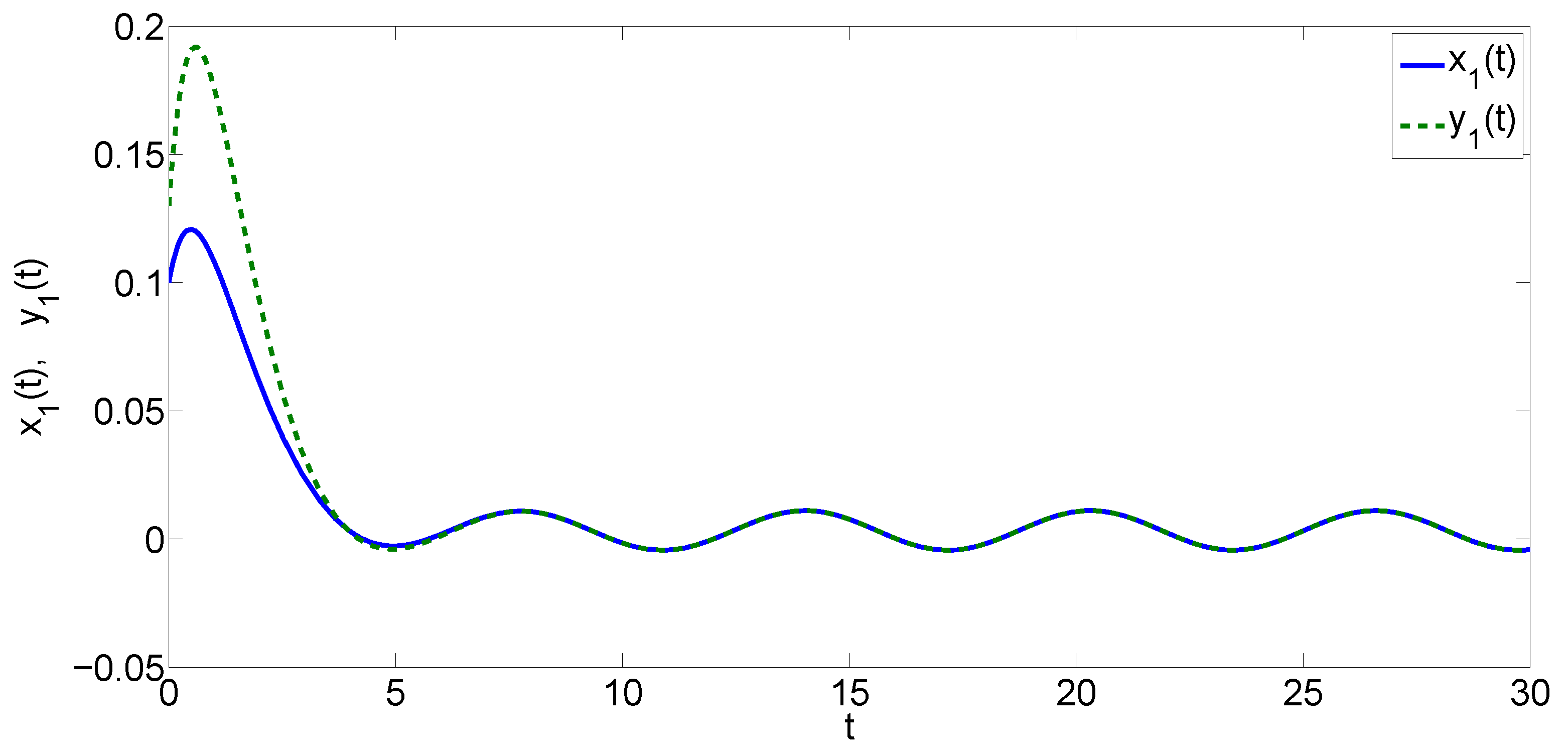
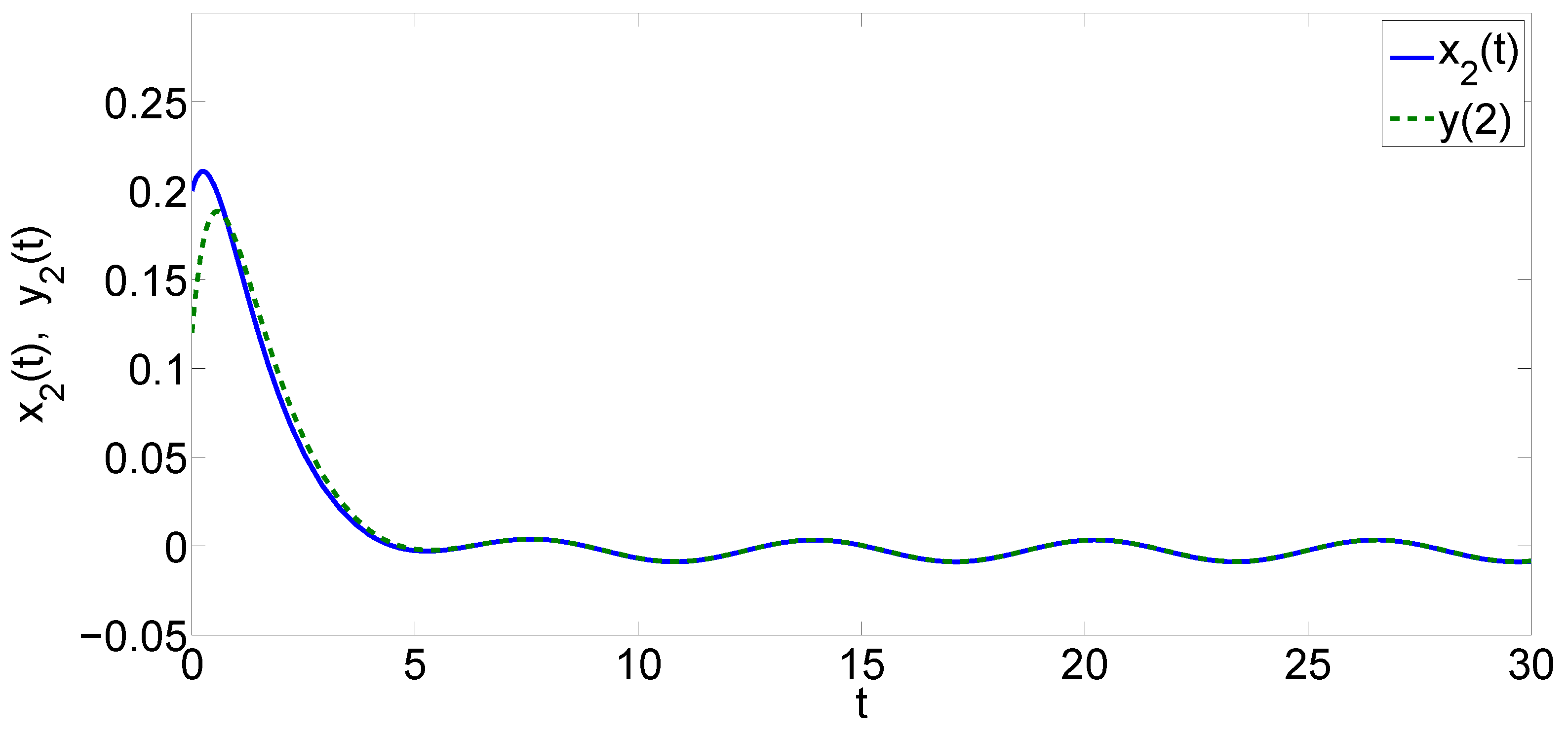
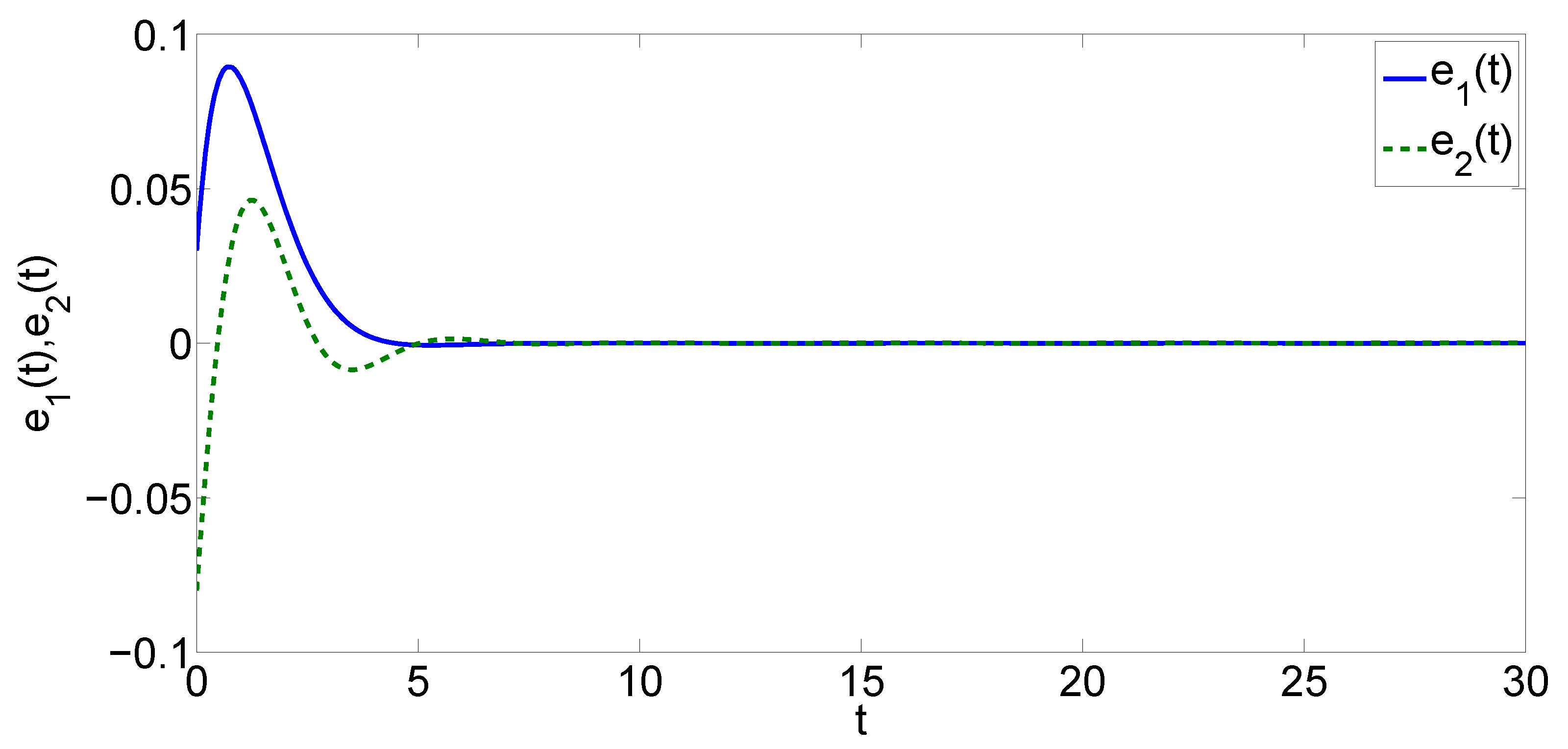
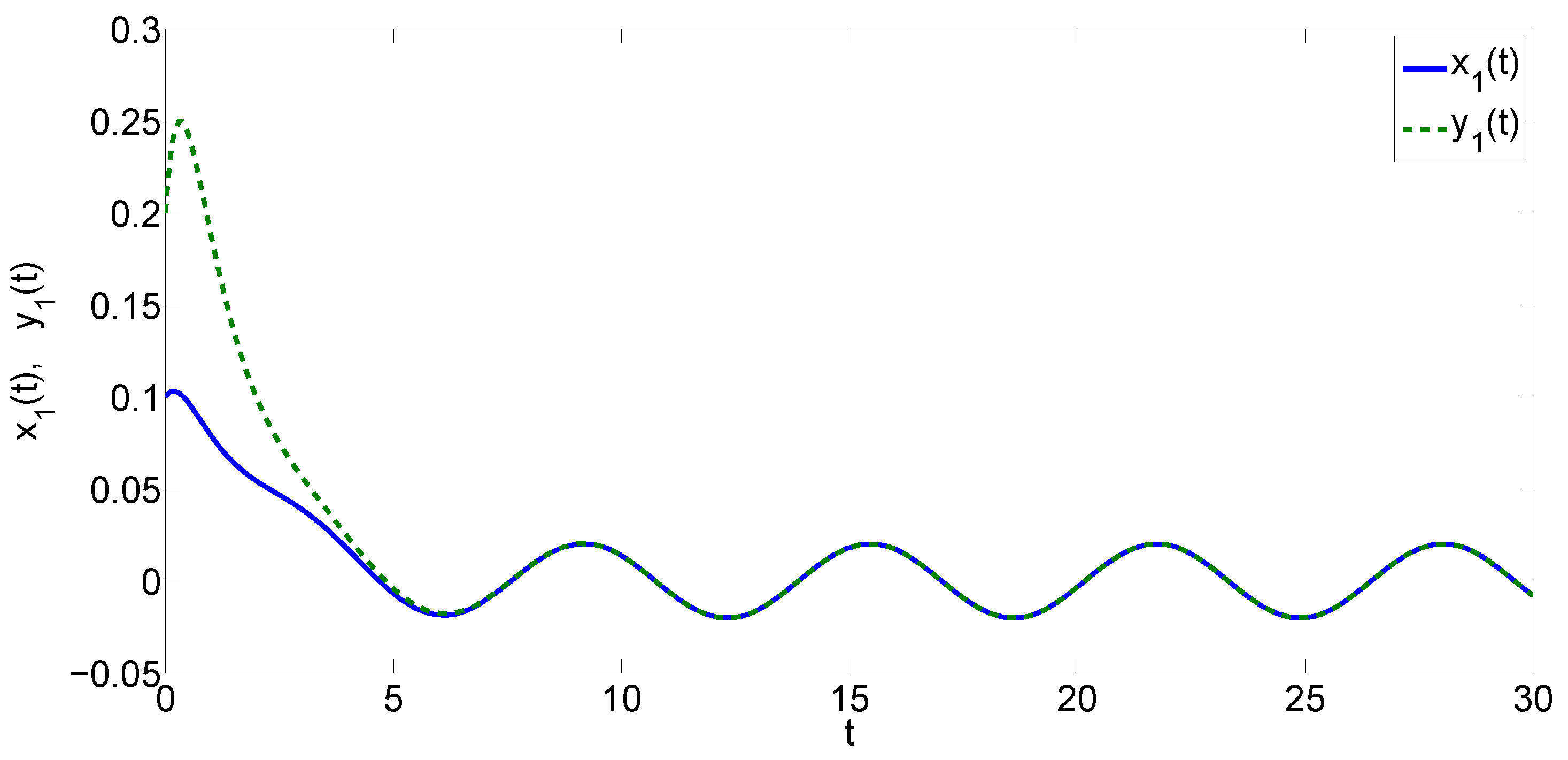
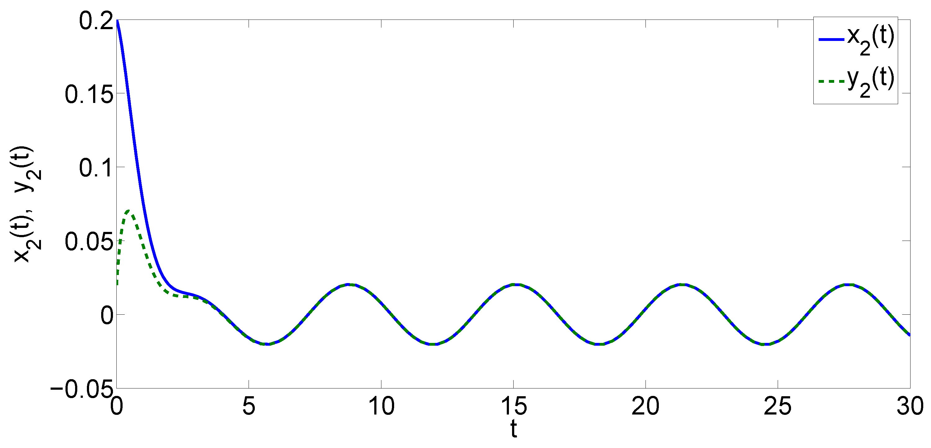
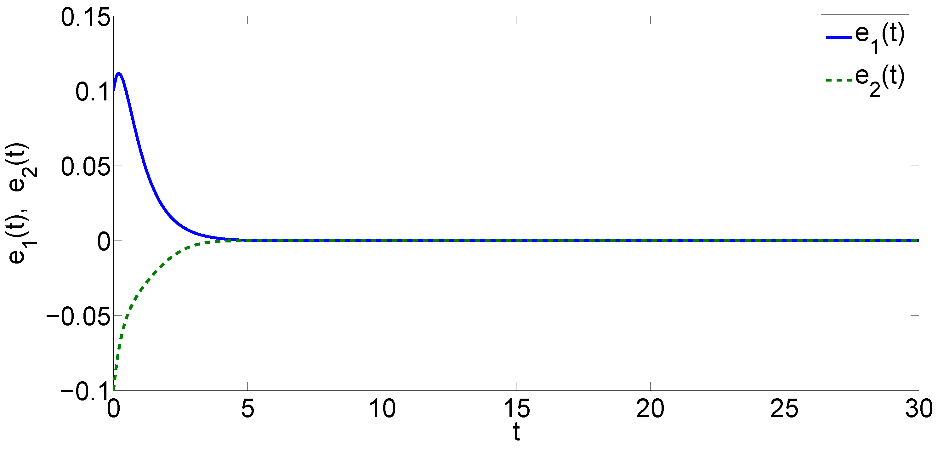
4. Numerical Examples

In this section, we give two numerical examples to illustrate our results.

Example 1.

Consider the following inertial neural networks with time delay ($n=2$)

$${\ddot{x}}_i\left(t\right)=-{\beta }_i{\dot{x}}_i\left(t\right)-{\alpha }_i{x}_i\left(t\right)+{\displaystyle \sum _{j=1}^2}{a}_{ij}{f}_j\left(x_j\left(t\right)\right)+{\displaystyle \sum _{j=1}^2}{b}_{ij}{f}_j\left(x_j(t-{\tau }_{ij})\right)+I_i\left(t\right).$$

(30)

The response system that is driven by Equation (30) is given as follows

$${\ddot{y}}_i\left(t\right)=-{\beta }_i{\dot{y}}_i\left(t\right)-{\alpha }_i{y}_i\left(t\right)+{\displaystyle \sum _{j=1}^2}{a}_{ij}{f}_j\left(y_j\left(t\right)\right)+{\displaystyle \sum _{j=1}^2}{b}_{ij}{f}_j\left(y_j(t-{\tau }_{ij})\right)+I_i\left(t\right)+u_i\left(t\right),$$

(31)

where $u_i\left(t\right)={\lambda }_i(y_i\left(t\right)-x_i\left(t\right)),{\lambda }_i>0,i=1,2.$ Set ${\alpha }_1=1.2,{\alpha }_2=1.5,{\beta }_1=2,{\beta }_2=2.5,$ $a_{11}=\frac{1}{32},a_{12}=-\frac{1}{32},a_{21}=-\frac{1}{64},a_{22}=-\frac{1}{64},$ $b_{11}=-\frac{1}{32},b_{12}=\frac{1}{64},b_{21}=\frac{1}{32},b_{22}=-\frac{1}{64},$ $f_i\left(x\right)=\frac{1}{8}sin\left(8x\right),I_i\left(t\right)=\frac{1}{16}exp(-t),{\tau }_{ij}=ln2,i,j=1,2.$ ${\lambda }_1=0.2,{\lambda }_2=0.4.$ Obviously, $|f_i\left(x\right)-f_i\left(y\right)|\le |x-y|,l_i=1,i=1,2.$

For numerical simulation, the initial condition is supposed to be $[{\phi }_{x1}\left(0\right),{\phi }_{x2}\left(0\right),{\psi }_{x1}\left(0\right)$, ${\psi }_{x2}\left(0\right),{\phi }_{y1}\left(0\right),{\phi }_{y2}\left(0\right),{\psi }_{y1}\left(0\right),{\psi }_{y2}\left(0\right)]=[0.1;0.2;0.1;0.1;0.13;0.12;0.25;0.3]$.

The simulation results are shown in Figure 1, Figure 2 and Figure 3.

Through simple calculation, we get the following results

$$-2{\alpha }_1+2{\lambda }_1+|2-{\alpha }_1-{\beta }_1+{\lambda }_1|+{\displaystyle \sum _{j=1}^2}(|a_{1j}|l_j+2|a_{j1}|l_1)+{\displaystyle \sum _{j=1}^2}{l}_1|b_{j1}|<-0.79<0,$$

$$2-2{\beta }_1+|2-{\alpha }_1-{\beta }_1+{\lambda }_1|+{\displaystyle \sum _{j=1}^2}|a_{1j}|l_j+{\displaystyle \sum _{j=1}^2}{l}_j|b_{1j}|<-0.89<0,$$

$$-2{\alpha }_2+2{\lambda }_2+|2-{\alpha }_2-{\beta }_2+{\lambda }_2|+{\displaystyle \sum _{j=1}^2}(|a_{2j}|l_j+2|a_{j2}|l_2)+{\displaystyle \sum _{j=1}^2}{l}_2|b_{j2}|<-0.38<0,$$

$$2-2{\beta }_2+|1-{\alpha }_2-{\beta }_2+{\lambda }_2|+{\displaystyle \sum _{j=1}^2}|a_{2j}|l_j+{\displaystyle \sum _{j=1}^2}{l}_j|b_{2j}|<-1.29<0.$$

By Theorem 1, the systems in Equations (30) and (31) are globally exponentially synchronized. Clearly, this consequence is coincident with the results of numerical simulation.

Example 2.

We consider the following inertial neural networks with time delay ($n=2$)

$${\ddot{x}}_i\left(t\right)=-{\beta }_i{\dot{x}}_i\left(t\right)-{\alpha }_i{x}_i\left(t\right)+{\displaystyle \sum _{j=1}^2}{a}_{ij}{f}_j\left(x_j\left(t\right)\right)+{\displaystyle \sum _{j=1}^2}{b}_{ij}{f}_j\left(x_j(t-{\tau }_{ij})\right)+I_i\left(t\right).$$

(32)

The response system that is driven by Equation (32) is given as follows

$${\ddot{y}}_i\left(t\right)=-{\beta }_i{\dot{y}}_i\left(t\right)-{\alpha }_i{y}_i\left(t\right)+{\displaystyle \sum _{j=1}^2}{a}_{ij}{f}_j\left(y_j\left(t\right)\right)+{\displaystyle \sum _{j=1}^2}{b}_{ij}{f}_j\left(y_j(t-{\tau }_{ij})\right)+I_i\left(t\right)+u_i\left(t\right),$$

(33)

where$u_i\left(t\right)=-{\lambda }_i(y_i\left(t\right)-x_i\left(t\right))-{\mu }_i(w_i\left(t\right)-z_i\left(t\right)),z_i\left(t\right)=\frac{d{x}_i\left(t\right)}{dt}+{\eta }_i{x}_i\left(t\right),$

$w_i\left(t\right)=\frac{d{y}_i\left(t\right)}{dt}+{\eta }_i{y}_i\left(t\right),i=1,2.$

${\alpha }_1=1,{\alpha }_2=2,{\beta }_1=3,{\beta }_2=2.5,$$a_{11}=\frac{1}{32},a_{12}=-\frac{1}{32},a_{21}=-\frac{1}{64},a_{22}=-\frac{1}{64},$

$b_{11}=-\frac{1}{32},b_{12}=\frac{1}{64},b_{21}=\frac{1}{32},b_{22}=-\frac{1}{64},$$f_i\left(x\right)=\frac{1}{8}sin\left(8x\right),I_i\left(t\right)=\frac{1}{16}exp(-t),$

${\tau }_{ij}=ln2,i,j=1,2.$${\eta }_1=0.6,{\eta }_2=0.8,{\mu }_1=1,{\mu }_2=2,{\lambda }_1=0.5,{\lambda }_2=0.4$

Obviously, $|f_i\left(x\right)-f_i\left(y\right)|\le |x-y|,i=1,2.$ We select $l_i=1.$ The initial condition is set to be $[{\phi }_{x1}\left(0\right),{\phi }_{x2}\left(0\right),{\psi }_{x1}\left(0\right),{\psi }_{x2}\left(0\right),{\phi }_{y1}\left(0\right),{\phi }_{y2}\left(0\right),{\psi }_{y1}\left(0\right),{\psi }_{y2}\left(0\right)]=[0.1;0.2;0.1;0.3;0.02;0.06;0.5;0.3]$. The simulation results of Example 2 are shown in Figure 4, Figure 5 and Figure 6.

We obtain the following results by calculation,

$$-2{\eta }_1+|{\alpha }_1+{\eta }_1^2-{\beta }_1{\eta }_1+{\lambda }_1-1|+{\displaystyle \sum _{j=1}^2}|a_{j1}|l_1+{\displaystyle \sum _{j=1}^1}{l}_1|b_{j1}|<-0.25<0,$$

$$-2{\beta }_1+2{\eta }_1-2{\mu }_1+|{\alpha }_1+{\eta }_1^2-{\beta }_1{\eta }_1+{\lambda }_1-1|+{\displaystyle \sum _{j=1}^2}|a_{j1}|l_1+{\displaystyle \sum _{j=1}^2}{l}_j|b_{1j}|e^{{\tau }_{1j}}<-4.55<0,$$

$$-2{\eta }_2+|{\alpha }_2+{\eta }_2^2-{\beta }_2{\eta }_2+{\lambda }_2-1|+{\displaystyle \sum _{j=1}^2}|a_{j2}|l_2+{\displaystyle \sum _{j=1}^2}{l}_i|b_{j2}|<-1.4<0,$$

$$-2{\beta }_2+2{\eta }_2-2{\mu }_2+|{\alpha }_2+{\eta }_2^2-{\beta }_2{\eta }_2+{\lambda }_2-1|+{\displaystyle \sum _{j=1}^2}|a_{j2}|l_2+{\displaystyle \sum _{j=1}^2}{l}_j|b_{2j}|e^{{\tau }_{2j}}<-7.2<0.$$

Thus, the conditions in Theorem 2 are satisfied. Then, the system in Equation (33) globally exponentially synchronizes with the system in Equation (32). Obviously, the conclusion from Theorem 2 is consistent with the numerical simulation results.

5. Conclusions

In this paper, we study the inertial neural networks with time delays, where ${\beta }_i$ is the damping coefficient. By employing the Lyapunov functional method, two exponential synchronization have been derived for the drive and response systems, which are useful in practice. These two sufficient conditions complement each other to be applied in different cases. Two examples have shown their effectiveness.

References

1. Zhang, X.; Wen, B.; Zhao, C. Theoretical, numerical and experimental study on synchronization of three identical exciters in a vibrating system. Chin. J. Mech. Eng. 2013, 26, 746–757. [Google Scholar] [CrossRef]
2. Lian, H.; Xiao, S.; Wang, Z.; Zhang, X.; Xiao, H. Further results on sampled-data synchronization control for chaotic neural networks with actuator saturation. Neurocomputing 2019, in press. [Google Scholar] [CrossRef]
3. Xiao, S.; Lian, H.; Teo, K.; Zeng, H.; Zhang, X. A new Lyapunov functional approach to sampled-data synchronization control for delayed neural networks. J. Frankl. Inst. 2018, 355, 8857–8873. [Google Scholar] [CrossRef]
4. Chung, S.J.; Slotine, J.J.E. Cooperative robot control and synchronization of Lagrangian systems. In Proceedings of the IEEE Conference on Decision & Control, New Orleans, LA, USA, 12–14 December 2007. [Google Scholar]
5. Weifa, P.; Dezong, Z. Speed Synchronization of Multi Induction Motors with Total Sliding Mode Control. In Proceedings of the 2010 Asia-Pacific Power & Energy Engineering Conference, Chengdu, China, 28–31 March 2010. [Google Scholar]
6. Rooks, B.W. Software synchronization for radial forging machine manipulators. Ind. Robot Int. J. 1996, 23, 19–23. [Google Scholar] [CrossRef]
7. Liu, Z.; Liu, S.; Huang, M. Influence Factors Research on Control Performance of Synchronous Control System for Giant Forging Hydraulic. Press Forg. Stamp. Technol. 2010, 35, 68–72. [Google Scholar]
8. Sun, H.; Chiu, T.C. Motion synchronization for dual-cylinder electrohydraulic lift systems. IEEE/ASME Trans. Mechatron. 2002, 7, 171–181. [Google Scholar]
9. Al-Mahbashi, G.; Noorani, M.S.M.; Bakar, S.A. Projective lag synchronization in drive-response dynamical networks with delay coupling via hybrid feedback control. Nonlinear Dyn. 2015, 82, 1569–1579. [Google Scholar] [CrossRef]
10. Zhou, L.; She, J.; Zhou, S.; Li, C. Compensation for state-dependent nonlinearity in a modified repetitive-control system. Int. J. Robust Nonlin. Control 2018, 28, 213–226. [Google Scholar] [CrossRef]
11. Zhou, L.; She, J.; Zhou, S. Robust H control of an observer-based repetitive-control system. J. Frankl. Inst. 2018, 355, 4952–4969. [Google Scholar] [CrossRef]
12. Zhou, W.; Zhu, Q.; Shi, P. Adaptive Synchronization for Neutral-Type Neural Networks with Stochastic Perturbation and Markovian Switching Parameters. IEEE Trans. Cybern. 2014, 44, 2848–2860. [Google Scholar] [CrossRef] [PubMed]
13. Yang, J.; Zhou, W.; Shi, P.; Yang, X.; Zhou, X.; Su, H. Adaptive synchronization of delayed Markovian switching neural networks with Lvy noise. Neurocomputing 2015, 156, 231–238. [Google Scholar] [CrossRef]
14. Li, X.; Song, S. Research on synchronization of chaotic delayed neural networks with stochastic perturbation using impulsive control method. Commun. Nonlinear Sci. Numer. Simul. 2014, 19, 3892–3900. [Google Scholar] [CrossRef]
15. Sun, W.; Wang, S.; Wang, G. Lag synchronization via pinning control between two coupled networks. Nonlinear Dyn. 2015, 79, 2659–2666. [Google Scholar] [CrossRef]
16. Wai, R.J.; Muthusamy, R. Fuzzy-neural-network inherited sliding-mode control for robot manipulator including actuator dynamics. IEEE Trans. Neural Netw. Learn. Syst. 2013, 24, 274–287. [Google Scholar]
17. Zhang, B.; Han, Q.; Zhang, X.; Yu, X. Sliding mode control with mixed current and delayed states for offshore steel jacket platform. IEEE Trans. Control Syst. Technol. 2014, 22, 1769–1783. [Google Scholar] [CrossRef]
18. Zhang, B.; Han, Q.; Zhang, X. Recent advances in vibration control of offshore platforms. Nonlinear Dyn. 2017, 89, 755–771. [Google Scholar] [CrossRef]
19. Andrievsky, B.; Fradkov, A.L.; Liberzon, D. Robustness of Pecora-Carroll synchronization under communication constraints. Syst. Control Lett. 2018, 111, 27–33. [Google Scholar] [CrossRef]
20. Badcock, K.L.; Westervelt, R.M. Dynamics of simple electronic neural networks. Phys. D 1987, 28, 305–316. [Google Scholar] [CrossRef]
21. Horikawa, Y.O. Bifurcation and stabilization of oscillations in ring neural networks with inertia. Phys. D 2009, 238, 2409–2418. [Google Scholar] [CrossRef]
22. Zhang, X.-M.; Han, Q.-L.; Wang, Z.; Zhang, B.-L. Neuronal state estimation for neural networks with two additive time-varying delay components. IEEE Trans. Cybern. 2017, 47, 3184–3194. [Google Scholar] [CrossRef] [PubMed]
23. Zhang, H.; Wang, Z.; Liu, D. A comprehensive review of stability analysis of continuous-time recurrent neural networks. IEEE Trans. Neural Netw. Learn. Syst. 2014, 25, 1229–1262. [Google Scholar] [CrossRef]
24. Zhang, X.; Han, Q.; Ge, X.; Ding, D. An overview of recent developments in Lyapunov-Krasovskii functionals and stability criteria for recurrent neural networks with time-varying delays. Neurocomputing 2018, 313, 392–401. [Google Scholar] [CrossRef]
25. Zhang, X.-M.; Han, Q.-L. Global asymptotic stability analysis for delayed neural networks using a matrix-based quadratic convex approach. Neural Netw. 2014, 54, 57–69. [Google Scholar] [CrossRef] [PubMed]
26. Xiao, S.; Xu, L.; Zeng, H.; Teo, K. Improved stability criteria for discrete-time delay systems via novel summation inequalities. Int. J. Control Autom. Syst. 2018, 16, 1592–1602. [Google Scholar] [CrossRef]
27. Zhang, X.-M.; Han, Q.-L.; Seuret, A.; Gouaisbaut, F.; He, Y. Overview of recent advances in stability of linear systems with time-varying delays. IET Control Theory Appl. 2019, 13, 1–16. [Google Scholar] [CrossRef]
28. Wang, J.; Zhang, X.; Han, Q. Event-triggered generalized dissipativity filtering for neural networks with time-varying delays. IEEE Trans. Neural Netw. Learn. Syst. 2016, 27, 77–88. [Google Scholar] [CrossRef] [PubMed]
29. Ke, Y.; Miao, C. Stability and existence of periodic solutions in inertial BAM neural networks with time delay. Neural Comput. Appl. 2013, 23, 1089–1099. [Google Scholar]
30. Ke, Y.; Miao, C. Stability analysis of inertial Cohen-Grossberg -type neural networks with time delays. Neurocomputing 2013, 117, 196–205. [Google Scholar] [CrossRef]
31. Ke, Y.; Miao, C. Exponental stability of periodic solutions for inertial Cohen-Grossberg-type neural, networks. Neural Netw. World. 2014, 4, 377–394. [Google Scholar] [CrossRef]
32. Ke, Y.; Miao, C. Exponential Stability of Periodic Solutions for Inertial Type BAM Cohen-Grossberg Neural Networks. Abstr. Appl. Anal. 2014, 2014, 857341. [Google Scholar]
33. Li, X.; Li, X.; Hu, C. Some new results on stability and synchronization for delayed inertial neural networks based on non-reduced order method. Neural Netw. 2017, 96, 91–100. [Google Scholar] [CrossRef] [PubMed]
34. Cao, J.; Wan, Y. Matrix measure strategies for stability and synchronization of inertial BAM neural network with time delays. Neural Netw. 2014, 53, 165–172. [Google Scholar] [CrossRef] [PubMed]
35. Lakshmanan, S.; Prakash, M.; Lim, C.P. Synchronization of an Inertial Neural Network With Time-Varying Delays and Its Application to Secure Communication. IEEE Trans. Neural Netw. Learn. Syst. 2018, 29, 195–207. [Google Scholar] [CrossRef] [PubMed]
36. Prakash, M.; Balasubramaniam, P.; Lakshmanan, S. Synchronization of Markovian jumping inertial neural networks and its applications in image encryption. Neural Netw. 2016, 83, 86–93. [Google Scholar] [CrossRef] [PubMed]
37. Rakkiyappan, R.; Premalatha, S. Chandrasekar, A. Stability and synchronization analysis of inertial memristive neural networks with time delays. Cogn. Neurodyn. 2016, 10, 437–451. [Google Scholar] [CrossRef] [PubMed]
38. Ruimei, Z.; Deqiang, Z.; Park, J.H. Quantized Sampled-Data Control for Synchronization of Inertial Neural Networks With Heterogeneous Time-Varying Delays. IEEE Trans. Neural Netw. Learn. Syst. 2018, 29, 1–11. [Google Scholar]
Figure 1. The synchronization trajectories between the state x 1 ( t ) of the drive system in Equation (30) and the state y 1 ( t ) of the response system in Equation (31) in Example 1.
Electronics 08 00356 g001
Figure 2. The synchronization trajectories between the state x 2 ( t ) of the drive system in Equation (30) and the state y 2 ( t ) of the response system in Equation (31) in Example 1.
Electronics 08 00356 g002
Figure 3. Evolution of synchronization errors e 1 ( t ) , e 2 ( t ) in Example 1.
Electronics 08 00356 g003
Figure 4. The synchronization trajectories between the state x 1 ( t ) of the drive system in Equation (32) and the state y 1 ( t ) of the response system in Equation (33) in Example 2.
Electronics 08 00356 g004
Figure 5. The synchronization trajectories between the state x 2 ( t ) of the drive system in Equation (32) and the state y 2 ( t ) of the response system in Equation (33) in Example 2.
Electronics 08 00356 g005
Figure 6. Evolution of synchronization errors e 1 ( t ) , e 2 ( t ) in Example 2.
Electronics 08 00356 g006