
A Swell Neural Network Algorithm for Solving Time-Varying Path Query Problems with Privacy Protection
Abstract
:1. Introduction
- The SNN algorithm can help to find multiple paths at once, including the shortest paths. This is difficult to achieve with other algorithms under time-varying conditions.
- For privacy protection, a scheme was designed with an encrypted index that effectively prevents the leakage of user information.
- Theoretical analyses and contrasting experimental results prove the efficiency, security, and accuracy of the algorithm.
2. Preliminaries
2.1. Definition of Time-Varying Path Query
2.2. Model of a Time-Varying Network Query
- Te encrypted with the ORE key
- Pst encrypted with the public secret key of RSA-1.
- (s, t, Ts) encrypted with the AES key
- Tu encrypted with the ORE key and the AES key
- f is the plaintext representing the number of paths queried.
3. Construction of the SNN
3.1. Design of the SNN Algorithm
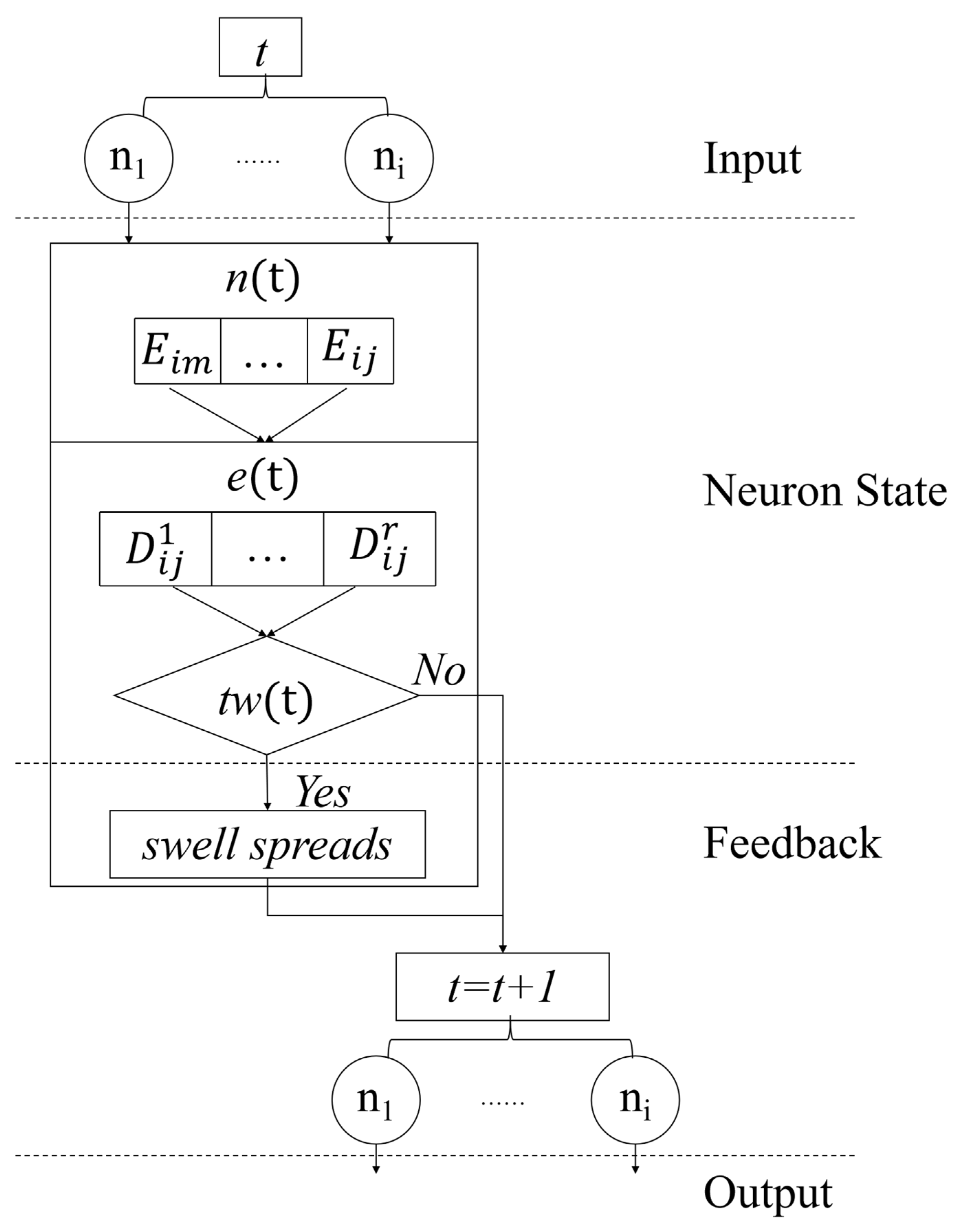
- Input: The input swells come from the predecessor nodes.
- Neuron state: The neuron state consists of three parts: nodes, edges, and time windows. The functions n(t), e(t) and tw(t) represent the processing of the node, edge, and time window, respectively, and t represents the current time.For , the successor set can be defined as , where the length of represents the number of swells from to .The predecessor set can be defined similarly.For edge , the time set collects the arrival times of for which no swell is currently formed.For time window , represents the set of key-value pairs for arrival and available times when no swell is formed.
- Feedback: The swells spread along the edge in the time window for which the available time ck satisfies the cost , and ck is computed as follows:
- Output: The output swells continue to spread to the successor nodes.
- Initialize the graph as Algorithm 2.
- Activate the start node directly as Algorithm 3.
- Iterate over the successor edges of the start node as Algorithm 4 to spread ripples.
- Iterate over all nodes over time to activate the nodes as Algorithm 4 until the target node is activated. The path can be obtained if the current time is within the maximum time range. Otherwise, no path meets the requirements.
| Algorithm 1 Encrypted Index Construction (EIC) |
| Input: |
| Output: |
| Initialize as Algorithm 2. |
| Initialize as Algorithm 3. |
| while and do |
| for do |
| Try to activate as Algorithm 4. |
| if has been changed do |
| as Algorithm 5. |
| end if |
| end while |
| Encrypt each path with and . |
| Algorithm 2 Graph Initialization (GI) |
| Input: |
| Output: |
| for do |
| for do |
| end for |
| end for |
| return G |
| Algorithm 3 Start Node Initialization (SI) |
| Input: |
| Output: |
| for do |
| for do |
| . |
| end for |
| end for |
| Algorithm 4 Node Activation (NA) |
| Input: |
| Output: |
| if or : |
| for do |
| Spread as Algorithm 6 |
| end for |
| end if |
| Algorithm 5 Add Paths (AP) |
| Input: |
| Output: |
| if do |
| if |
| if do |
| break |
| end if |
| end if |
| else |
| for do |
| AP(Algorithm 5) |
| end for |
| end if |
| Algorithm 6 Swell Spreading (SS) |
| Input: |
| Output: |
| //Initialize the set of arrival times to be deleted from |
| for |
| key = Perform time window determination as Algorithm 7 |
| if do |
| end if |
| end for |
| for : |
| Delete from |
| Delete (,*) from |
| , and as Algorithm 3 |
| end for |
| Algorithm 7 Time Window Determination (TD) |
| Input: . |
| Output: |
| // Initialize the arrival time to be deleted from |
| for (the key-value pair set of ) |
| if do |
| else if do |
| end if |
| if do |
| end if |
| end for |
| return de |
3.2. An Example of the SNN Algorithm
- The user, say Bob, generates a unique secret key for AES , distinguished from those of other users to prevent leakage from others.
- Bob→Cloud: Send , which is encrypted by
- Bob→Cloud: Encrypt as an encrypted query according to Definition 4, encrypt with the AES key and encrypt 5 with the ORE key and the AES key .
- Cloud: Decrypt the query with , use to find f matching encrypted indices, and compare the second part of the encrypted index with 5. If the former is not greater, the item meets the query.
- Cloud→Bob: Query the result encrypted with .
- Bob: Decrypt the information with KAES and then with SkRSA1 to obtain the query result .
3.3. Complexity
3.4. Security
4. Experiments
5. Conclusions
Funding
Data Availability Statement
Conflicts of Interest
Abbreviations
| Symbols | Explanation |
| The graph | |
| The start node | |
| The target node | |
| The departure time | |
| The arrival time | |
| The private key of RSA-1 | |
| The public key of RSA-1 | |
| The private key of RSA-2 | |
| The public key of RSA-2 | |
| The key of AES | |
| The key of ORE | |
| The upper limit of the arrival time | |
| One path from to | |
| The paths set from to | |
| The length of | |
| The edge from to | |
| The time window of the edge from to | |
| The rth time window of the edge from to | |
| The lower boundary of | |
| The upper boundary of | |
| The cost of | |
| The cost of | |
| The cost of in real time | |
| The predecessor of | |
| The successor of node i | |
| The predecessor edge set of | |
| The successor edge set of | |
| The number of nodes | |
| The number of paths queried | |
| The number of time windows of each edge | |
| The father set of | |
| The arrival time set of with that swell has not spread to next node currently | |
| The son set of |
References
- References Ge, X.; Yu, J.; Zhang, H.; Bai, J.; Fan, J.; Xiong, N.N. SPPS: A search pattern privacy system for approximate shortest distance query of encrypted graphs in iiot. IEEE Trans. Syst. Man Cybern. Syst. 2022, 52, 136–150. [Google Scholar]
- Zhou, Y.; Lu, Y.; Lv, L. Grid-based non-uniform probabilistic roadmap-based agv path planning in narrow passages and complex environments. Electronics 2024, 13, 225–240. [Google Scholar] [CrossRef]
- Huang, W.; Gao, L. A time wave neural network framework for solving time-dependent project scheduling problems. IEEE Trans. Neural Netw. Learn. Syst. 2020, 31, 274–283. [Google Scholar] [CrossRef] [PubMed]
- Cao, N.; Yang, Z.; Wang, C.; Ren, K.; Lou, W. Privacy-preserving query over encrypted graph-structured data in cloud computing. In Proceedings of the 2011 31st International Conference on Distributed Computing Systems, Minneapolis, MN, USA, 20–24 June 2011; pp. 105–117. [Google Scholar]
- Memon, I.; Arain, Q.A. Dynamic path privacy protection framework for continuous query service over road networks. World Wide Web 2017, 20, 639–672. [Google Scholar] [CrossRef]
- Shang, H.; Zhang, Y.; Lin, X.; Yu, J.X. Taming verification hardness: An efficient algorithm for testing subgraph isomorphism. Proc. Vldb Endow. 2008, 1, 364–375. [Google Scholar] [CrossRef]
- Gouda, K.; Hassaan, M. Compressed feature-based filtering and verification approach for subgraph search. In Proceedings of the EDBT’13: Proceedings of the 16th International Conference on Extending Database Technology, Genoa, Italy, 18–22 March 2013; pp. 201–213. [Google Scholar]
- Lin, W.; Xiao, X.; Cheng, J.; Bhowmick, S.S. Efficient algorithms for generalized subgraph query processing. In Proceedings of the CIKM’12: Proceedings of the 21st ACM international conference on Information and knowledge management, Maui, HI, USA, 29 October–2 November 2012; Association for Computing Machinery: New York, NY, USA, 2012; pp. 325–352. [Google Scholar]
- Meng, X.; Kamara, S.; Nissim, K.; Kollios, G.N. GRECS: Graph encryption for approximate shortest distance queries. In Proceedings of the CCS’15: Proceedings of the 22nd ACM SIGSAC Conference on Computer and Communications Security, Denver, CO, USA, 12–16 October 2015; Association for Computing Machinery: New York, NY, USA, 2015; pp. 25–42. [Google Scholar]
- Xie, P.; Xing, E. CryptGraph: Privacy Preserving Graph Analytics on Encrypted Graph. arXiv 2014, arXiv:1409.5021. [Google Scholar]
- Cooke, K.L.; Halsey, E. The shortest route through a network with time-dependent internodal transit times. J. Math. Anal. Appl. 1966, 14, 493–498. [Google Scholar] [CrossRef]
- Frigioni, D.; Marchetti-Spaccamela, A.; Nanni, U. Fully dynamic output bounded single source shortest path problem. In Proceedings of the SODA’96: Proceedings of the Seventh Annual ACM-SIAM Symposium on Discrete Algorithms, Atlanta, GA, USA, 28–30 January 1996; pp. 212–221. [Google Scholar]
- Ramalingam, G.; Reps, T. An incremental algorithm for a generalization of the shortest-path problem. J. Algorithms 1996, 21, 267–305. [Google Scholar] [CrossRef]
- King, V. Fully dynamic algorithms for maintaining all-pairs shortest paths and transitive closure in digraphs. In Proceedings of the 40th Annual Symposium on Foundations of Computer Science, New York, NY, USA, 17–19 October 1999; pp. 81–89. [Google Scholar]
- Demetrescu, C.; Italiano, G. A new approach to dynamic all pairs shortest paths. J. ACM 2004, 51, 968–992. [Google Scholar] [CrossRef]
- Liu, C.; Zhu, L.; He, X.; Chen, J. Enabling privacy-preserving shortest distance queries on encrypted graph data. IEEE Trans. Dependable Secur. Comput. 2021, 18, 192–204. [Google Scholar] [CrossRef]
- Ghosh, E.; Kamara, S.; Tamassia, R. Efficient graph encryption scheme for shortest path queries. In Proceedings of the ASIA CCS’21: ACM Asia Conference on Computer and Communications Security, Hong Kong, China, 7–11 June 2021; pp. 31–43. [Google Scholar]
- Sun, F.; Yu, J.; Ge, X.; Yang, M.; Kong, F. Constrained top-k nearest fuzzy keyword queries on encrypted graph in road network. Comput. Secur. 2021, 111, 430–442. [Google Scholar] [CrossRef]
- Wu, B.; Chen, X.; Wu, Z.; Zhao, Z.; Mei, Z.; Zhang, C. Privacy-guarding optimal route finding with support for semantic search on encrypted graph in cloud computing scenario. Wirel. Commun. Mob. Comput. 2021, 2021, 6617959. [Google Scholar] [CrossRef]
- Zhang, D.; Liu, Y.; Liu, A.; Mao, X.; Li, Q. Efficient path query processing through cloud-based mapping services. IEEE Access 2017, 5, 12963–12973. [Google Scholar] [CrossRef]
- Huang, W.; Sun, M.; Zhu, L.; Oh, S.; Pedrycz, W. Deep fuzzy min-max neural network: Analysis and design. IEEE Trans. Neural Netw. Learn. Syst. 2022. [Google Scholar] [CrossRef]
- Huang, W.; Wang, Y.; Zhu, L. A time impulse neural network framework for solving the minimum path pair problems of the time-varying network. IEEE Trans. Knowl. Data Eng. 2023, 35, 7681–7692. [Google Scholar] [CrossRef]
- Zhang, C.; Luo, X.; Liang, J.; Liu, X.; Zhu, L.; Guo, S. POTA: Privacy-preserving online multi-task assignment with path planning. IEEE Trans. Mob. Comput. 2023, 4, 1–13. [Google Scholar] [CrossRef]
- Shen, M.; Ma, B.; Zhu, L.; Mijumbi, R.; Du, X.; Hu, J. Cloud-based approximate constrained shortest distance queries over encrypted graphs with privacy protection. IEEE Trans. Inf. Forensics Secur. 2018, 13, 940–953. [Google Scholar] [CrossRef]
- Huang, W.; Wang, J.; Wang, W. A time-delay neural network for solving time-dependent shortest path problem. Neural Netw. 2017, 90, 21–28. [Google Scholar] [CrossRef]
- Tahat, N.; Tahat, A.A.; Abu-Dalu, M. A new RSA public key encryption scheme with chaotic maps. Int. J. Electr. Comput. Eng. 2020, 10, 1430–1437. [Google Scholar] [CrossRef]
- Huang, X.; Wang, W. A novel and efficient design for an rsa cryptosystem with a very large key size. IEEE Trans. Circuits Syst. 2015, 62, 972–976. [Google Scholar] [CrossRef]
- Masoumi, M. Novel hybrid cmos/memristor implementation of the aes algorithm robust against differential power analysis attack. IEEE Trans. Circuits Syst. 2020, 67, 1314–1318. [Google Scholar] [CrossRef]
- Peyrin, T. Practical Order-Revealing Encryption with Limited Leakage; Springer: Berlin/Heidelberg, Germany, 2016; Volume 9783, pp. 474–493. [Google Scholar]
- Zhang, C.; Zhao, M.; Liang, J.; Fan, Q.; Zhu, L.; Guo, S. NANO: Cryptographic enforcement of readability and editability governance in blockchain databases. IEEE Trans. Dependable Secur. Comput. 2023, 4, 1–14. [Google Scholar] [CrossRef]
- Hu, C.; Zhang, C.; Lei, D.; Wu, T.; Liu, X.; Zhu, L. Achieving privacy-preserving and verifiable support vector machine training in the cloud. IEEE Trans. Inf. Forensics Secur. 2023, 18, 3476–3491. [Google Scholar] [CrossRef]
- Zhu, D.; Sun, J. A new algorithm based on dijkstra for vehicle path planning considering intersection attribute. IEEE Access 2021, 9, 19761–19775. [Google Scholar] [CrossRef]
- Sang, Y.; Lv, J.; Qu, H.; Yi, Z. Shortest path computation using pulse-coupled neural networks with restricted autowave. Knowl.-Based Syst. 2016, 114, 1–11. [Google Scholar] [CrossRef]


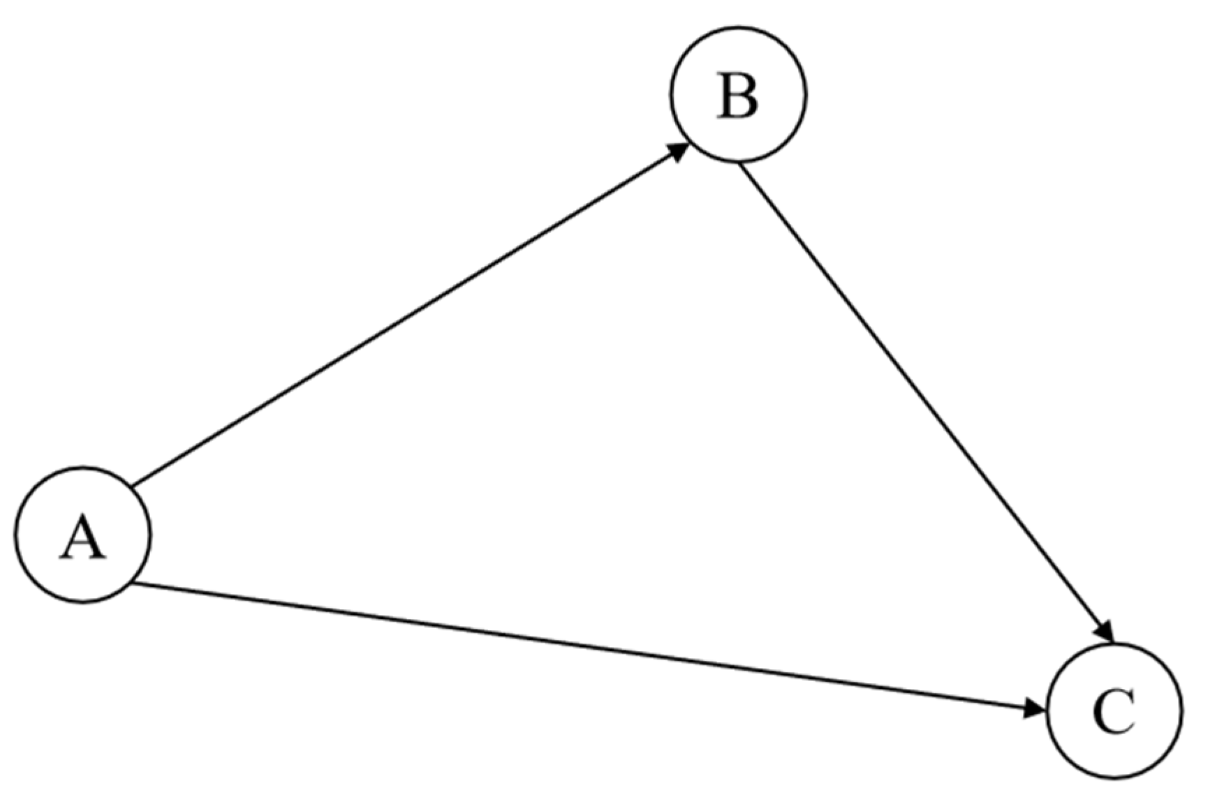
| Node | Edge | Time Window | Cost |
|---|---|---|---|
| A | AB | [0, 3 | 1 |
| [3, + | 2 | ||
| AC | [0, 2 | 2 | |
| [3, + | 4 | ||
| B | BC | [0, 3 | 2 |
| [3, + | 3 |
| node | |||||||
| edge | - | ||||||
| Time window | - | ||||||
| (a) Running SI () | |||||||
| None | |||||||
| - | |||||||
| - | |||||||
| (b) Running NA (t = 1) | |||||||
| Si | |||||||
| Fi | |||||||
| - | |||||||
| - | |||||||
| (c) Running NA () | |||||||
| Si | |||||||
| Fi | |||||||
| Pij | - | ||||||
| - | |||||||
| (d) Running AP | |||||||
| paths | |||||||
| (e) Running NA () | |||||||
| Si | |||||||
| Fi | None | ||||||
| Pij | - | ||||||
| - | |||||||
| (f) Running AP | |||||||
| paths | |||||||
| Dataset | Nodes | Edges | Time Windows | Tu | Storage |
|---|---|---|---|---|---|
| Dataset 1 | 50 | 115 | 230 | 50 | 4 KB |
| Dataset 2 | 100 | 230 | 460 | 200 | 7 KB |
| Dataset 3 | 500 | 1244 | 2488 | 500 | 44 KB |
| Dataset 4 | 1000 | 2493 | 4986 | 1000 | 92 KB |
| Dataset | Dijkstra | PCNN | TDNN |
|---|---|---|---|
| Dataset 1 | 0.001 | 0.001 | 0.001 |
| Dataset 2 | 0.004 | 0.003 | 0.003 |
| Dataset 3 | 0.10 | 0.08 | 0.08 |
| Dataset 4 | 0.26 | 0.31 | 0.24 |
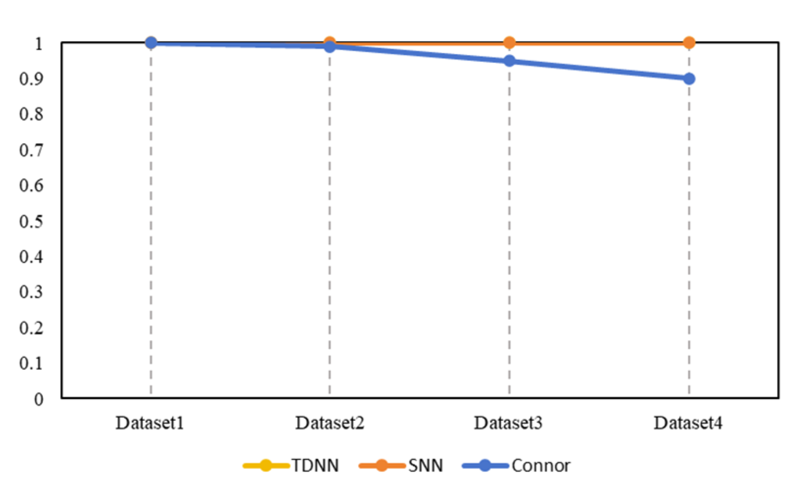
| Dataset | SNN | TDNN | Connor |
|---|---|---|---|
| Dataset 1 | 0.03 | 0.08 | 0.05 |
| Dataset 2 | 0.12 | 0.53 | 0.1 |
| Dataset 3 | 3.13 | 64.10 | 0.8 |
| Dataset 4 | 18.72 | 225.75 | 8.9 |
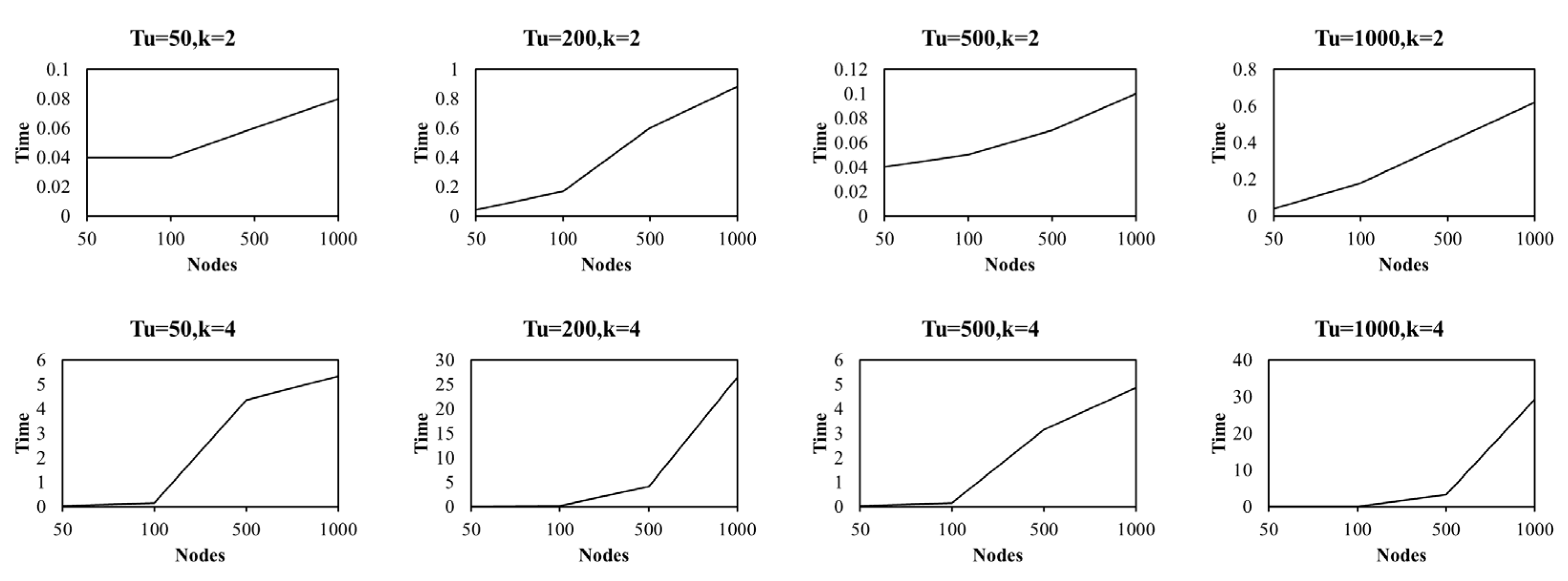
| Dataset | Tu = 50 s | Tu = 200s | Tu = 500 s | Tu = 1000 s |
|---|---|---|---|---|
| Dataset 1 | 0.04 | 0.04 | 0.03 | 0.03 |
| Dataset 2 | 0.04 | 0.17 | 0.16 | 0.16 |
| Dataset 3 | 0.06 | 0.60 | 4.36 | 4.10 |
| Dataset 4 | 0.08 | 0.88 | 5.34 | 26.41 |
| Dataset | Tu = 50 s | Tu = 200 s | Tu = 200 s | Tu = 200 s |
|---|---|---|---|---|
| Dataset 1 | 0.04 | 0.04 | 0.04 | 0.04 |
| Dataset 2 | 0.05 | 0.18 | 0.15 | 0.15 |
| Dataset 3 | 0.07 | 0.4 | 3.16 | 3.32 |
| Dataset 4 | 0.10 | 0.62 | 4.86 | 29.18 |
Disclaimer/Publisher’s Note: The statements, opinions and data contained in all publications are solely those of the individual author(s) and contributor(s) and not of MDPI and/or the editor(s). MDPI and/or the editor(s) disclaim responsibility for any injury to people or property resulting from any ideas, methods, instructions or products referred to in the content. |
© 2024 by the author. Licensee MDPI, Basel, Switzerland. This article is an open access article distributed under the terms and conditions of the Creative Commons Attribution (CC BY) license (https://creativecommons.org/licenses/by/4.0/).
Share and Cite
Zhao, M. A Swell Neural Network Algorithm for Solving Time-Varying Path Query Problems with Privacy Protection. Electronics 2024, 13, 1248. https://doi.org/10.3390/electronics13071248
Zhao M. A Swell Neural Network Algorithm for Solving Time-Varying Path Query Problems with Privacy Protection. Electronics. 2024; 13(7):1248. https://doi.org/10.3390/electronics13071248
Chicago/Turabian StyleZhao, Man. 2024. "A Swell Neural Network Algorithm for Solving Time-Varying Path Query Problems with Privacy Protection" Electronics 13, no. 7: 1248. https://doi.org/10.3390/electronics13071248