Multisource Sparse Inversion Localization with Long-Distance Mobile Sensors

Abstract

To address the threat posed by unknown signal sources within Mobile Crowd Sensing (MCS) systems to system stability and to realize effective localization of unknown sources in long-distance scenarios, this paper proposes a unilateral branch ratio decision algorithm (UBRD). This approach addresses the inadequacies of traditional sparse localization algorithms in long-distance positioning by introducing a time–frequency domain composite block sparse localization model. Given the complexity of localizing unknown sources, a unilateral branch ratio decision scheme is devised. This scheme derives decision thresholds through the statistical characteristics of branch residual ratios, enabling adaptive control over iterative processes and facilitating multisource localization under conditions of remote blind sparsity. Simulation results indicate that the proposed model and algorithm, compared to classic sparse localization schemes, are more suitable for long-distance localization scenarios, demonstrating robust performance in complex situations like blind sparsity, thereby offering broader scenario adaptability.

1. Introduction

With the advancement of digital technologies such as smartphones, Mobile Crowd Sensing (MCS) technologies [1,2,3] and wireless sensor network positioning [4] are increasingly applied in fields like communications and the Internet of Things (IoT) [5,6,7]. Traditional positioning techniques often rely on static wireless sensor networks (WSNs) [8], which are costly to construct and lack mobility. In contrast, positioning technologies based on MCS [9] offer the advantages of low cost and broad applicability, possessing significant appeal and competitive advantages.

Positioning technologies based on MCS can be categorized into two main types: range-based and range-free positioning [10]. Range-free positioning algorithms [11,12,13] do not require the measurement of distances, signal strengths, or angle information between terminals within the environment as model inputs. Classical algorithms include the centroid algorithm, channel-aware positioning, Distance Vector-Hop (DV-Hop) algorithm [14], and convex programming, among others. On the other hand, range-based positioning algorithms conduct raw signal collection through MCS, extracting feature information parameters to construct mathematical equations for solving the target’s location. Classical algorithms in this category include techniques based on received signal strength (RSS), Angle of Arrival (AoA), Time of Arrival (ToA), and Time Difference of Arrival (TDoA) [15,16,17,18].

However, the aforementioned methods all possess certain limitations. While range-free positioning techniques have lower hardware requirements, they suffer from poor positioning accuracy. Conversely, range-based positioning techniques offer higher accuracy, but technologies such as TDoA and ToA have higher hardware demands and are not well-suited for MCS scenarios. Moreover, in MCS environments, the application of multiple access technologies [19] introduces scenarios with multiple coexisting and co-frequency signal sources. Existing technologies have conducted specific research [20,21] on positioning in multisource environments, but most struggle to accurately locate signal sources in such complex scenarios.

In recent years, with the advent of compressive sensing theory [22], research [23] has introduced a multisource positioning technique based on compressive sensing, providing a novel research paradigm for multi-target positioning [24]. This positioning technology relies solely on the sparsity of received signal strengths and receiver location information to locate multiple signal sources, enabling the positioning of several simultaneous co-frequency signal sources. One study [25] has rigorously demonstrated the efficacy of the sparse optimization problem formulation for positioning and proven that the sensing matrix satisfies the Restricted Isometry Property (RIP).

Existing sparse positioning techniques still have limitations; traditional sparse positioning methods based on MCS can only position signal sources within the coverage area of MCS devices [26], and they are incapable of performing long-distance sparse positioning on signal sources outside the coverage area. Additionally, most current compressive sensing techniques require a known sparsity level [27] as a prior condition for iterative process control, which is challenging to obtain in practical MCS scenarios as the exact number of signal sources is often unknown.

With further research into compressive sensing technologies, such as block sparsity [28,29], scholars have proposed and validated their RIPs. However, in the field of sparse positioning, there has yet to be research specifically addressing positioning problems based on block sparsity, indicating room for further exploration in sparse positioning.

In view of the current research deficiencies, this paper proposes a block sparsity system model constructed based on time-domain and energy-domain for addressing the problem of long-distance sparse positioning in MCS scenarios. Furthermore, it introduces a unilateral branch ratio decision (UBRD) algorithm based on the block sparsity system model to achieve blind sparsity adaptive iterative control.

The research work in this paper is as follows:

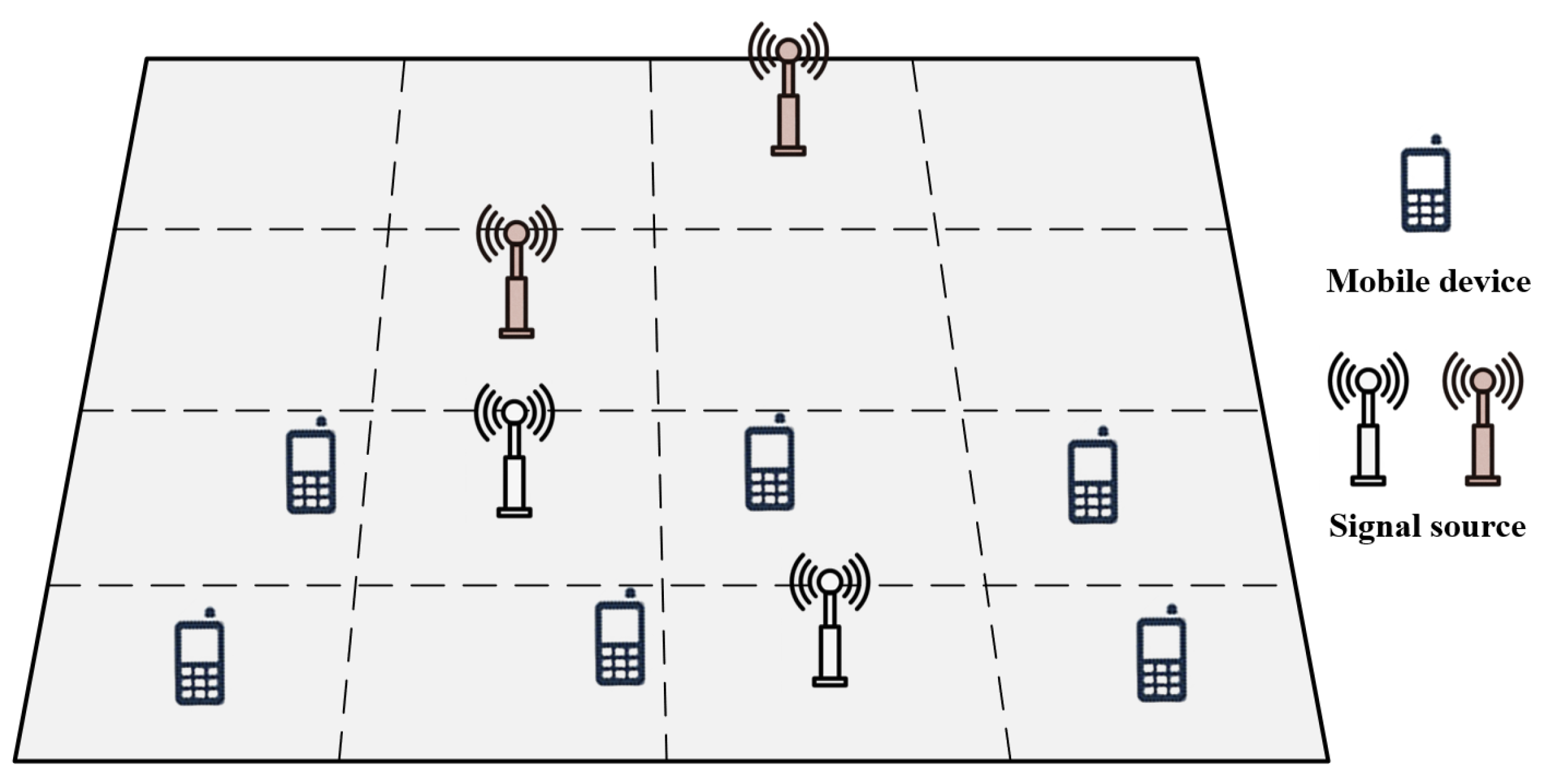
• Based on the MCS context, this study implements long-distance sparse positioning by constructing and solving a block sparsity model synthesized from time and energy domains. Compared to the aforementioned sparse inversion positioning algorithms, the block sparsity-based positioning algorithm can achieve simultaneous co-frequency multisource positioning within the periphery of the sensor network.
• Within the framework of sparse positioning, this study introduces an adaptive iterative recovery by unilateral detection of branch residuals during the iteration process and provides expressions for false alarm probability and decision thresholds. Compared to traditional compressive sensing algorithms, the UBRD algorithm can adaptively control the iterative process under blind sparsity conditions.
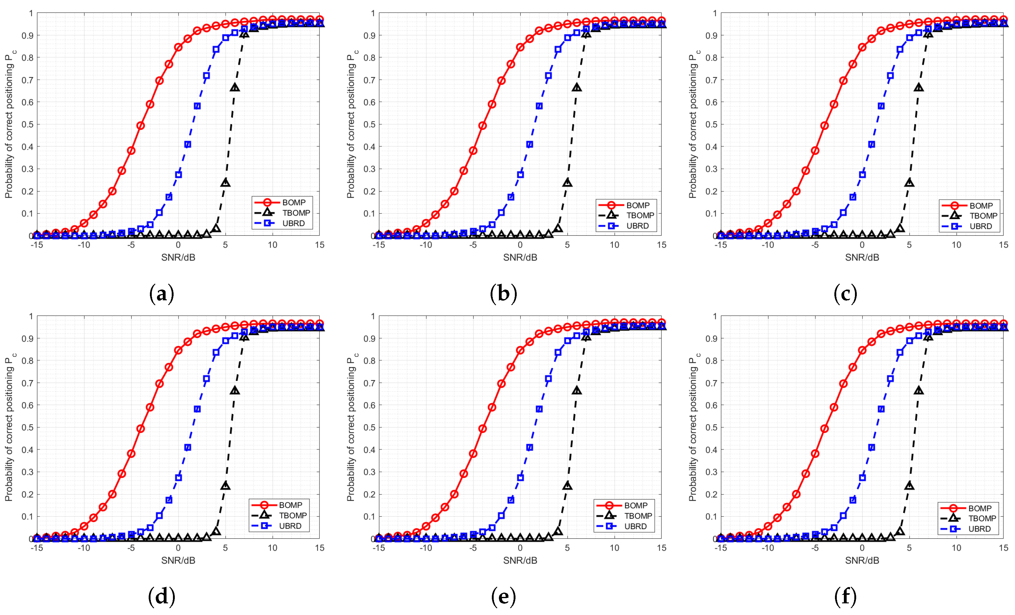
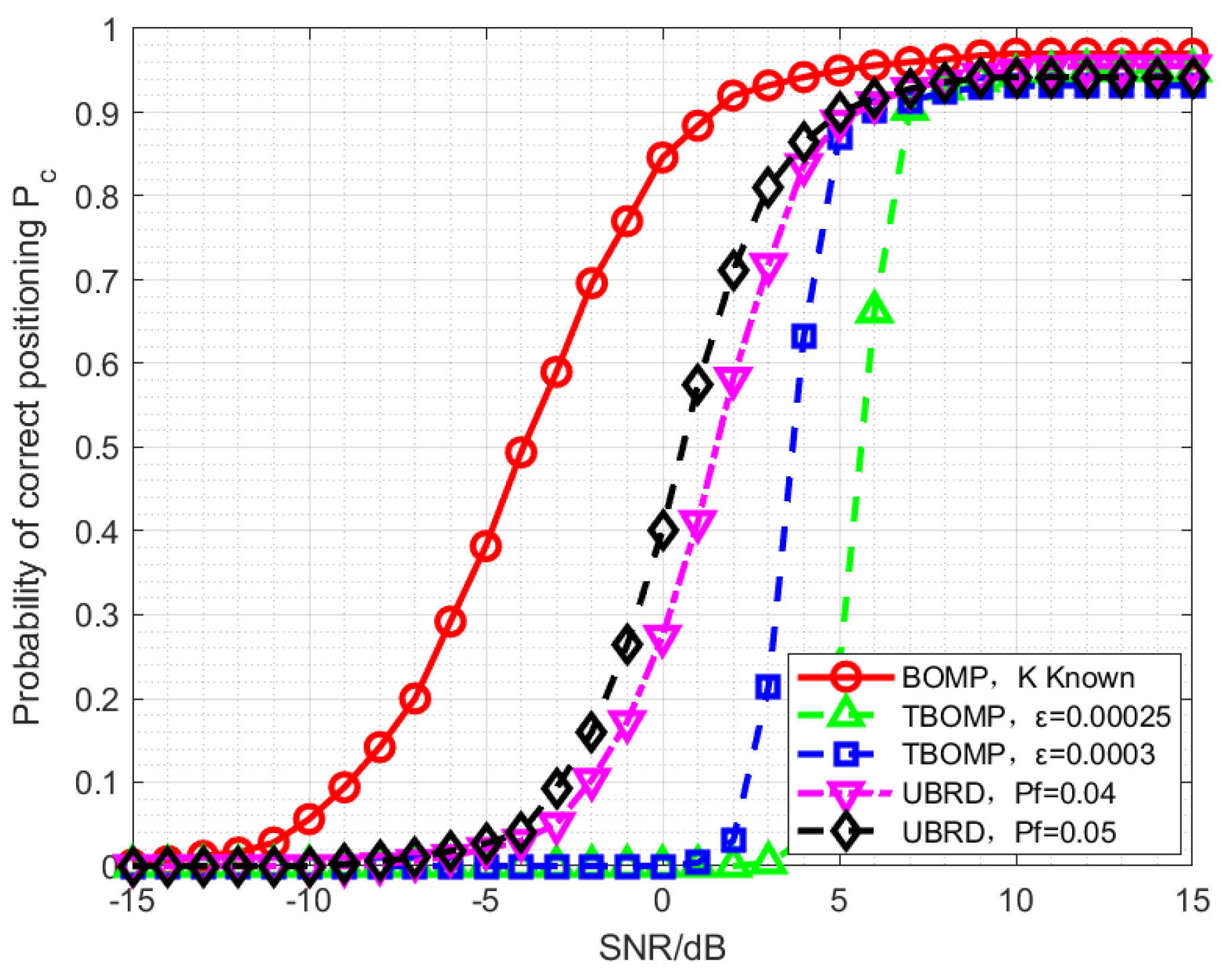
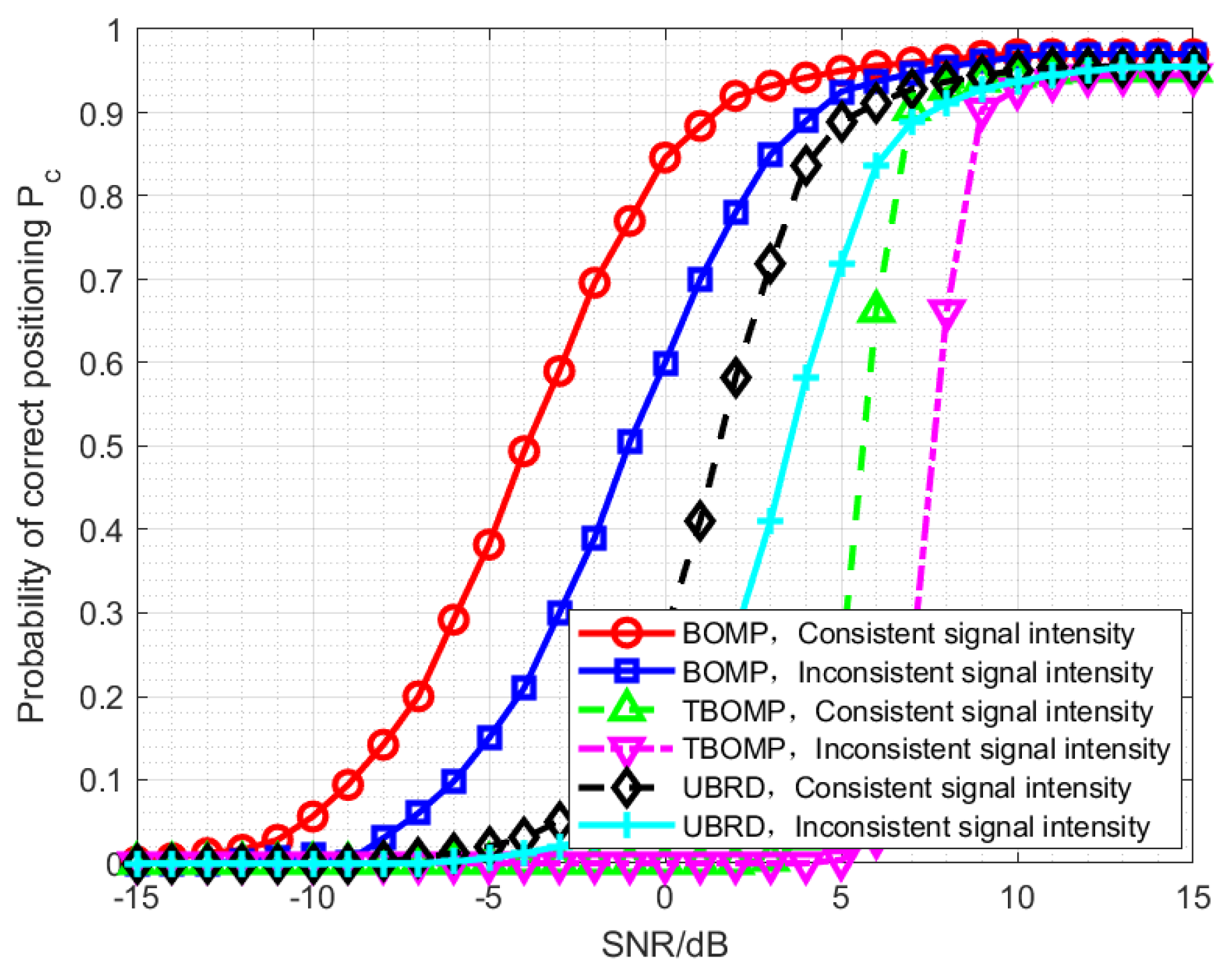
• Simulation results for different algorithms under various scenarios indicate that the block sparsity-based sparse positioning technology can achieve long-distance simultaneous co-frequency multisource positioning and has broader scenario adaptability. Under conditions of unknown sparsity, the UBRD algorithm demonstrates superior performance compared to algorithms that make decisions based on energy thresholds.

2. MCS Positioning and Problem Description

To facilitate the subsequent elaboration of the proposed unilateral branch ratio decision (UBRD) algorithm in later sections, we first revisit the traditional framework of MCS sparse positioning. Subsequently, we discuss the issues associated with long-distance positioning within this framework and introduce the block sparsity positioning model. Building on this model, we then present the iterative control problem inherent in the process.

2.1. MCS Sparse Localization Framework and Issues

In the context of MCS scenarios, multisource sparse localization is depicted in the lower half of Figure 1, where the source of the signal is positioned within the enveloping range of sensors. Under the conventional framework for sparse localization, the sensor coverage space is subjected to grid partitioning. This approach utilizes the grid positions as approximations for estimating the target location. Assume that in this scenario, there are K signal sources and M mobile devices, with the position of the ith mobile device denoted as $m_i=[x_{m_i},y_{m_i}]$. The space is divided into N grids, with the position of the jth grid represented as $n_j=[x_{n_j},y_{n_j}]$.

The scenario of multisource perception based on ubiquitous passive radar is depicted in Figure 1. It consists of M passive radars and K radiating sources.

In the MCS localization scenario, within the same frequency f, the number of signal sources is limited. The number of grid units and signal sources satisfy the condition $N\gg K$. Hence, the positions of the signal sources exhibit sparsity in the spatial domain. According to compressive sensing theory, a sparse model can be constructed to solve the multisource localization problem. The model is formulated as follows:

Without loss of generality, consider the scene area uniformly discretized into N square grids. Among them, M passive radars are randomly distributed in the scene, and K signal sources are randomly distributed within the grids. Since $N\gg K$, the positional information of signal sources exhibits sparsity within the target scene.

$$\mathbf{y}=\mathbf{Ax}+\mathbf{n},$$

(1)

where $\mathbf{y}$ represents the received signal vector. $\mathbf{A}$ is an $M\ast N$ dimensional sensing matrix, $\mathbf{x}$ is the sparse vector of signal sources, and $\mathbf{n}$ denotes Gaussian noise within the scene. The detailed meanings of the aforementioned parameters are as follows:

(1)

Received Signal Vector $\mathbf{y}$

$\mathbf{y}={\left[y_1,y_2,\dots ,y_M\right]}^T$ represents the received signal vector composed of the received signal strength (RSS) from M mobile devices, where each element $y_i$ signifies the received signal strength value $P_i$ of the ith mobile device at frequency f. $P_i$ denotes the sum of energy from all signal sources attenuated and reaching mobile device i.

(2)

Signal Source Sparse Vector $\mathbf{x}$

$\mathbf{x}={\left[x_1,x_2,\dots ,x_N\right]}^T$ represents the sparse vector of signal sources at frequency f within the scene, where each element $x_j$ signifies the signal source energy intensity within the jth grid region. The majority of elements in $\mathbf{x}$ possess a value of 0, rendering $\mathbf{x}$ a sparse vector.

(3)

Sensing Matrix $\mathbf{A}$

Given that $P_i$ represents the summation of energy attenuated from $\mathbf{x}$ reaching the ith location, namely:

$$P_i=\sum _{j=1}^N{E}_{ij}{x}_j,$$

(2)

where $E_{ij}$ denotes the energy attenuation coefficient, representing the energy intensity loss between the ith mobile device location and the jth grid location. $E_{ij}$ is obtained through the free-space loss formula, $F_{ij}$, with the specific formula outlined as follows:

$$F_{ij}=20log(4\pi /c)+20log\left(d_{ij}\right)+20log\left(f\right)-G_r-G_t,$$

(3)

where c represents the speed of light, $d_{ij}=\sqrt{{\left(x_{m_i}-x_{n_j}\right)}^2+{\left(y_{m_i}-y_{n_j}\right)}^2}$ signifies the distance between the ith mobile device location and the jth grid location, and $G_t$ and $G_r$ denote the antenna gains of the signal source and the mobile device, respectively. The energy attenuation coefficient $E_{ij}={10}^{\left(F_{ij}/\phantom{F_{ij}20}20\right)}$ can be obtained based on Equation (3).

The sensing matrix $\mathbf{A}$ is composed of energy attenuation coefficients $E_{ij}$, and $\mathbf{A}$ is specifically represented as follows:

$$\mathbf{A}={\left[\begin{array}{c}{\mathbf{A}}_1\\ {\mathbf{A}}_2\\ ⋮\\ {\mathbf{A}}_N\end{array}\right]}^T=\left[\begin{array}{cccc}{E}_{11}& E_{12}& \dots & E_{1N}\\ E_{21}& E_{22}& \dots & E_{2N}\\ ⋮& ⋮& \ddots & ⋮\\ E_{M1}& E_{M2}& \dots & E_{MN}\end{array}\right].$$

(4)

Combining the aforementioned derivations, the localization problem based on MCS can be equivalently formulated as solving $\mathbf{y}=\mathbf{Ax}+\mathbf{n}$. Due to sparsity, this equation can be solved using compressive sensing algorithms. In the classic MCS-based localization scenario, the Orthogonal Matching Pursuit (OMP) algorithm can be employed to solve the sparse equation. The algorithmic procedure for the OMP is illustrated in Algorithm 1.

Algorithm 1 The OMP Algorithm

Input:  mobile device reception vector $\mathbf{y}$; sensor matrix $\mathbf{A}$. Initialize:  number of iterations $\tau =0$; residual vector ${\mathbf{r}}^{\mathbf{0}}=\mathbf{y}$; support set $Sup{p}^0=\varnothing$; sensing matrix reconstruction $\widehat{\mathbf{A}}=\varnothing$; reconstruction of signal source vectors ${\mathbf{x}}^{\mathbf{0}}=\varnothing$; sparsity K. while  $\tau <K$    1: $\tau =\tau +1$.    2: $B^{\tau }=\underset{j\notin Sup{p}^{\tau -1}}{argmax}\left|〈{\mathbf{r}}^{\tau -1},{\mathbf{A}}_j〉\right|$.    3: $Sup{p}^{\tau }=Sup{p}^{\tau -1}\cup B^{\tau }$.    4: ${\widehat{\mathbf{A}}}^{\tau }=\left[{\widehat{\mathbf{A}}}^{\tau -1},{\mathbf{A}}_{B^{\tau }}\right]$.    5: ${\mathbf{x}}^{\tau }=arg\underset{{\mathbf{x}}^{\tau }}{min}{∥\mathbf{y}-{\widehat{\mathbf{A}}}^{\tau }{\mathbf{x}}^{\tau }∥}_2^2$.    6: ${\mathbf{r}}^{\tau }=\mathbf{y}-{\widehat{\mathbf{A}}}^{\tau }{\mathbf{x}}^{\tau }$. Output:  location information support set $Supp$.

Following the aforementioned steps, the positional support set $Supp$ can be acquired to enable multisource localization. However, this method is applicable exclusively to scenarios where the signal source is surrounded by sensors, as depicted in the traditional framework. In instances where the signal source, exemplified by the red signal sources in Figure 1, is located outside the sensor envelopment range, this methodology proves to be inapplicable. The results of employing this method for locating signal sources situated outside the sensor envelopment range are presented in subsequent chapters.

2.2. The Block Sparse Long-Range Localization Model and Its Associated Issues

The block sparse long-range localization model is akin to the classical sparse localization model in its approach. This model involves gridding the target space and approximating the target’s position using grid locations. In this scenario, there are K signal sources and M mobile devices, where the position of the ith mobile device is denoted as $m_i=[x_{m_i},y_{m_i}]$, and the number of grids in the signal source area is N, with the jth grid position represented as $n_j=[x_{n_j},y_{n_j}]$. Unlike the classical sparse localization model, this model integrates temporal and energy domains, where both the measured signal and sparse signal sources are in the frequency domain. The specific formulation of the block sparse long-range localization model is as follows:

$$\mathbf{Y}=\mathbf{AX}+\mathbf{N},$$

(5)

where $\mathbf{Y}$ represents the received signal vector. $\mathbf{A}$ stands for the sensing matrix, $\mathbf{X}$ denotes the signal source block sparse vector, and $\mathbf{N}$ represents the Gaussian noise within the scene. In this scenario, the mobile devices receive not just simple power intensities but rather discrete signals of length L. The detailed interpretations of the aforementioned parameters are as follows:

(1)

The received signal vector $\mathbf{Y}$

$\mathbf{Y}$ represents the signals received from a collective set of M mobile devices, with each individual mobile device capturing a discrete signal block of length L. The received signal vector $\mathbf{Y}$ is characterized by a total length of $L_M$, precisely $L_M=M\ast L$. The specific representation of vector $\mathbf{Y}$ is detailed as follows:

$$\mathbf{Y}={\left[\underset{{\mathbf{Y}}_1^T}{\underbrace{Y_0,\cdots ,Y_{L-1}}},\underset{{\mathbf{Y}}_2^T}{\underbrace{Y_L,\cdots ,Y_{2L-1}}},\cdots ,\underset{{\mathbf{Y}}_M^T}{\underbrace{Y_{L_M-L-1},\cdots ,Y_{L_M-1}}}\right]}^T,$$

(6)

where ${\mathbf{Y}}_i^T$ represents the frequency-domain received signal of the ith mobile device. This received signal is the superposition of frequency-domain transformations at the mobile device location, resulting from all signal source signals after energy attenuation and time delay.

(2)

The signal source block sparse vector $\mathbf{X}$

$\mathbf{X}$ represents the output vector of signal sources within N grids, where each signal source emits a frequency-domain discrete signal block of length L. $\mathbf{X}$ is characterized by a total length of $L_N$, precisely $L_N=N\ast L$. The specific representation of vector $\mathbf{X}$ is detailed as follows:

$$\mathbf{X}={\left[\underset{{\mathbf{X}}_1^T}{\underbrace{X_0,\cdots ,X_{L-1}}},\underset{{\mathbf{X}}_2^T}{\underbrace{X_L,\cdots ,X_{2L-1}}},\cdots ,\underset{{\mathbf{X}}_N^T}{\underbrace{X_{L_N-L-1},\cdots ,X_{L_N-1}}}\right]}^T,$$

(7)

where ${\mathbf{X}}_j^T$ represents the frequency-domain output vector of the jth signal source within the scene’s grid. In most grids, there are no signal sources present, thus the value for the corresponding block is 0, rendering ${\mathbf{X}}_j^T$ as a block sparse vector.

(3)

Sensing Matrix $\mathbf{A}$

The signal travels a certain distance to reach the mobile device, experiencing energy attenuation during propagation. Additionally, due to varying positions of different signal sources concerning the mobile device, there are differences in signal transmission distances. This results in the same signal reaching different mobile devices at different times. Based on the properties of Discrete Fourier Transform, the formula representing the frequency-domain signal received by the specific ith mobile device at the jth grid location is as follows:

$$\left(\begin{array}{c}{Y}_{\left(i-1\right)L-1}\\ Y_{\left(i-1\right)L}\\ ⋮\\ Y_{iL-1}\end{array}\right)=\left(\begin{array}{cccc}{A}_{ij0}& 0& \cdots & 0\\ 0& A_{ij1}& \cdots & 0\\ ⋮& ⋮& \ddots & ⋮\\ 0& 0& \cdots 0& A_{ijL-1}\end{array}\right)\left(\begin{array}{c}{X}_{\left(j-1\right)L-1}\\ X_{\left(j-1\right)L}\\ ⋮\\ X_{jL-1}\end{array}\right).$$

(8)

Equation (8) can be abbreviated as ${\mathbf{Y}}_{ij}={\mathbf{A}}_{ij}{\mathbf{X}}_j$, where ${\mathbf{Y}}_{ij}$ represents the frequency-domain signal obtained by the ith mobile device from the jth grid, ${\mathbf{X}}_j$ signifies the frequency-domain output vector of the signal source within the jth grid in the scenario, and ${\mathbf{A}}_{ij}$ denotes the sensing matrix between the two nodes. The specific construction of the aforementioned formula is detailed below.

$$\mathbf{x}\left[t-t_{ij}\right]\leftrightarrow \mathbf{X}\left[l\right]e^{-j2\pi l{t}_{ij}/\phantom{-j2\pi l{t}_{ij}L}L}.$$

(9)

From Equation (3), the energy attenuation coefficient $E_{ij}$ between nodes i and j can be derived. Combining this with Equation (9), the calculation of the element ${\mathrm{A}}_{ijl}$ in matrix ${\mathbf{A}}_{ij}$ is computed as follows:

$${\mathrm{A}}_{ijl}=E_{ij}\ast e^{-j2\pi l{t}_{ij}/\phantom{-j2\pi l{t}_{ij}L}L}.$$

(10)

In the long-distance localization model based on MCS, the ith mobile device is required to receive signals from all signal sources within the scene. The frequency-domain received signal for the ith node is expressed as follows:

$${\mathbf{Y}}_i=\sum _{j=1}^N{\mathbf{Y}}_{ij}=\sum _{j=1}^N{\mathbf{A}}_{ij}{\mathbf{X}}_j.$$

(11)

Expanding Equation (11) to encompass all mobile devices, we can derive the sensing matrix $\mathbf{A}$ as follows:

$$\mathbf{A}={\left[\begin{array}{c}{\mathbf{A}}_1\\ {\mathbf{A}}_2\\ ⋮\\ {\mathbf{A}}_N\end{array}\right]}^T=\left[\begin{array}{cccc}{\mathbf{A}}_{11}& {\mathbf{A}}_{12}& \cdots & {\mathbf{A}}_{1N}\\ {\mathbf{A}}_{21}& {\mathbf{A}}_{22}& \cdots & {\mathbf{A}}_{2N}\\ ⋮& ⋮& \ddots & ⋮\\ {\mathbf{A}}_{M1}& {\mathbf{A}}_{M2}& \cdots & {\mathbf{A}}_{MN}\end{array}\right].$$

(12)

Taking into account the derivations presented above, we can formulate the long-range block sparse localization model under the MCS framework as follows:

$$\left[\begin{array}{c}{\mathbf{Y}}_1\\ {\mathbf{Y}}_2\\ ⋮\\ {\mathbf{Y}}_M\end{array}\right]=\left[\begin{array}{cccc}{\mathbf{A}}_{11}& {\mathbf{A}}_{12}& \cdots & {\mathbf{A}}_{1N}\\ {\mathbf{A}}_{21}& {\mathbf{A}}_{22}& \cdots & {\mathbf{A}}_{2N}\\ ⋮& ⋮& \ddots & ⋮\\ {\mathbf{A}}_{M1}& {\mathbf{A}}_{M2}& \cdots & {\mathbf{A}}_{MN}\end{array}\right]\left[\begin{array}{c}\begin{array}{c}{\mathbf{X}}_1\\ {\mathbf{X}}_2\\ ⋮\end{array}\\ {\mathbf{X}}_N\end{array}\right]+\left[\begin{array}{c}\begin{array}{c}{\mathbf{N}}_1\\ {\mathbf{N}}_2\\ ⋮\end{array}\\ {\mathbf{N}}_N\end{array}\right],$$

(13)

where $\mathbf{Y}={\left[{\mathbf{Y}}_1,{\mathbf{Y}}_2,\dots ,{\mathbf{Y}}_M\right]}^T$ represents the combined vector of frequency-domain signals received by M mobile devices over a specified time period. $\mathbf{X}={\left[{\mathbf{X}}_1,{\mathbf{X}}_2,\dots ,{\mathbf{X}}_N\right]}^T$ corresponds to the vector of block coefficient signals for N grid regions. The sensing matrix $\mathbf{A}$ is formed by the signal transformation coefficients between the grid locations within the scene and the mobile devices, thereby constituting an overcomplete dictionary.

Similar to the OMP algorithm, the presented model can be solved using greedy algorithms such as BOMP. The detailed steps of the BOMP algorithm are outlined in Algorithm 2, as shown below.

Algorithm 2 The BOMP Algorithm

Input:  mobile device reception vector $\mathbf{Y}$; sensor matrix $\mathbf{A}$. Initialize:  number of iterations $\tau =0$; residual vector ${\mathbf{Y}}^{\mathbf{0}}=\mathbf{Y}$; support set $Sup{p}^0=\varnothing$; sensing matrix reconstruction $\widehat{\mathbf{A}}=\varnothing$; reconstruction of signal source vectors ${\mathbf{X}}^{\mathbf{0}}=\varnothing$; sparsity K. while  $\tau <K$    1: $\tau =\tau +1$.    2: $B^{\tau }=\underset{j\notin Sup{p}^{\tau -1}}{argmax}{∥{{\mathbf{A}}_j}^T{\mathbf{Y}}^{\tau -1}∥}_2$.    3: $Sup{p}^{\tau }=Sup{p}^{\tau -1}\cup B^{\tau }$.    4: ${\widehat{\mathbf{A}}}^{\tau }=\left[{\widehat{\mathbf{A}}}^{\tau -1},{\mathbf{A}}_{B^{\tau }}\right]$.    5: ${\mathbf{X}}^{\tau }=arg\underset{{\mathbf{X}}^{\tau }}{min}{∥\mathbf{Y}-{\widehat{\mathbf{A}}}^{\tau }{\mathbf{X}}^{\tau }∥}_2^2$.    6: ${\mathbf{Y}}^{\tau }=\mathbf{Y}-{\widehat{\mathbf{A}}}^{\tau }{\mathbf{X}}^{\tau }$. Output:  location information support set $Supp$.

Similar to traditional sparse algorithms, block sparse models are typically reconstructed using greedy algorithms through iterative processes. However, akin to the challenges faced by conventional sparse algorithms, many existing block sparse algorithms suffer from practical limitations in controlling the iterative process. Classical sparse algorithms utilize sparsity control in the iterative process, which exhibits favorable performance but necessitates knowledge of the number of signal sources within the scene as the sparsity parameter. Nevertheless, in practical localization scenarios, estimating the number of signal sources is often challenging.

Taking the Threshold-Based Orthogonal Matching Pursuit (TBOMP) algorithm as an example, some improved algorithms employ predetermined residual thresholds for iterative control. Such methods do not require prior knowledge of sparsity but do necessitate information about background noise. The algorithm is outlined in Algorithm 3.

Algorithm 3 The TBOMP Algorithm

Input:  mobile device reception vector $\mathbf{Y}$; sensor matrix $\mathbf{A}$. Initialize:  number of iterations $\tau =0$; residual vector ${\mathbf{Y}}^{\mathbf{0}}=\mathbf{Y}$; support set $Sup{p}^0=\varnothing$; sensing matrix reconstruction $\widehat{\mathbf{A}}=\varnothing$; reconstruction of signal source vectors ${\mathbf{X}}^{\mathbf{0}}=\varnothing$; preset threshold $\epsilon$. while  $\mathrm{norm}({\mathbf{Y}}^{\tau })>\epsilon$    1: $\tau =\tau +1$.    2: $B^{\tau }=\underset{j\notin Sup{p}^{\tau -1}}{argmax}{∥{{\mathbf{A}}_j}^T{\mathbf{Y}}^{\tau -1}∥}_2$.    3: $Sup{p}^{\tau }=Sup{p}^{\tau -1}\cup B^{\tau }$.    4: ${\widehat{\mathbf{A}}}^{\tau }=\left[{\widehat{\mathbf{A}}}^{\tau -1},{\mathbf{A}}_{B^{\tau }}\right]$.    5: ${\mathbf{X}}^{\tau }=arg\underset{{\mathbf{X}}^{\tau }}{min}{∥\mathbf{Y}-{\widehat{\mathbf{A}}}^{\tau }{\mathbf{X}}^{\tau }∥}_2^2$.    6: ${\mathbf{Y}}^{\tau }=\mathbf{Y}-{\widehat{\mathbf{A}}}^{\tau }{\mathbf{X}}^{\tau }$. Output:  location information support set $Supp$.

Due to the variability inherent in MCS scenarios, it is challenging for the TBOMP algorithm to achieve adaptive and effective iterative control. To address the aforementioned issues, this paper proposes a unilateral branch ratio decision (UBRD) algorithm. The UBRD algorithm employs a false alarm method to make decisions based on the branch residual ratio, thus achieving iterative control. For the sake of subsequent computations, the false alarm probability is defined as follows:

$$P_{fa}=Pr\{Supp\ne \mathbf{S}\},$$

(14)

where $Supp$ denotes the computed position support set, and $\mathbf{S}$ signifies the actual position support set, both representing the indices of signal source locations within N grid regions.The false alarm probability $P_{fa}$ signifies the probability of a mismatch between the inferred position support set and the actual position support set, which can be further divided into the probability of under-recovery and the probability of over-recovery.

Following the definition of the false alarm probability, the UBRD module is designed based on this probability. Within the iterative process of determining the position support set, this module achieves iterative control by examining whether the residual vector retains signal source components. In each iteration, it assesses the residual ratios among different branches to ascertain whether the iterative process has acquired a complete support set. This process can be summarized as a set of binary hypothesis testing problems:

$${\mathbf{Y}}^{\tau }=\left\{\begin{array}{cc}{\mathbf{A}}^{\tau }\mathbf{N},& G_{0,\tau }\\ {\mathbf{A}}^{\tau }\left(\mathbf{X}+\mathbf{N}\right),& G_{1,\tau },\end{array}\right.$$

(15)

where ${\mathbf{Y}}^{\tau }$ represents the residual vector, which corresponds to the residuals of mobile sensing nodes in the $\tau$th iteration process. ${\mathbf{A}}^{\tau }$ denotes the sensing matrix in the $\tau$th iteration, and the specific expressions for these two parameters are provided in the subsequent algorithm section. $\mathbf{X}$ represents the block sparse signal sources within the target area, and $\mathbf{N}$ signifies Gaussian white noise within the scene. $G_{0,\tau }$ represents the hypothesis in the $\tau$th iteration where the residual only contains noise components, indicating that the position information support set has been completely acquired and the iterative process should be terminated. $G_{1,\tau }$ represents the hypothesis in the $\tau$th iteration where the residual contains signal components, suggesting that the position information support set has not been fully acquired and the iterative process should continue.

3. Algorithm Design

In this section, we introduce the unilateral branch ratio decision (UBRD) algorithm based on the long-range localization model established in the previous section. We calculate the residual for each branch and investigate its statistical characteristics. Subsequently, we derive the expressions for false alarm probability and decision threshold.

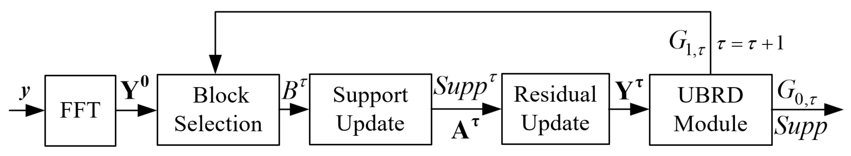
3.1. Algorithm Steps

As illustrated in Figure 2, this paper introduces the UBRD algorithm. Similar to the traditional sparse localization algorithms mentioned in the previous section, this algorithm is a greedy algorithm. It comprises four main steps:

• Most Relevant Block Selection: In the first step, the algorithm calculates the index of the most relevant block by comparing the sensing matrix with the received signal vector.
• Support Set Update: In the second step, the algorithm updates the position support set based on the index of the most relevant block, and consequently updates the sensing matrix.
• Residual Update: The third step involves updating the residual vector using the sensing matrix obtained in the previous step.
• UBRD Module: In the fourth step, the UBRD module adaptively controls the iterative process by adjusting the residual detection threshold based on a predefined false alarm probability.

The detailed steps of the UBRD algorithm proposed in this paper are presented in Algorithm 4.

Algorithm 4 The UBRD Algorithm

Input:  mobile device reception vector $\mathbf{Y}$; sensor matrix $\mathbf{A}$; false alarm rate of residual detection $P_{fa}$. Initialize:  number of iterations $\tau =0$; residual vector ${\mathbf{Y}}^{\mathbf{0}}=\mathbf{Y}$; support set $Sup{p}^0=\varnothing$; sensing matrix reconstruction $\widehat{\mathbf{A}}=\varnothing$; reconstruction of signal source vectors ${\mathbf{X}}^{\mathbf{0}}=\varnothing$. Repeat:       1: $\tau =\tau +1$.    2: $B^{\tau }=\underset{j\notin Sup{p}^{\tau -1}}{argmax}{∥{{\mathbf{A}}_j}^T{\mathbf{Y}}^{\tau -1}∥}_2/\phantom{{∥{{\mathbf{A}}_j}^T{\mathbf{Y}}^{\tau -1}∥}_2{∥{{\mathbf{A}}_j}^T{\mathbf{A}}_j∥}_2}{∥{{\mathbf{A}}_j}^T{\mathbf{A}}_j∥}_2$.    3: $Sup{p}^{\tau }=Sup{p}^{\tau -1}\cup B^{\tau }$; ${\widehat{\mathbf{A}}}^{\tau }=\left[{\widehat{\mathbf{A}}}^{\tau -1},{\mathbf{A}}_{B^{\tau }}\right]$.    4: ${\mathbf{X}}^{\tau }={\mathbf{A}}^{†}{\mathbf{Y}}^0$; ${\mathbf{A}}^{†}={\left({\left({\widehat{\mathbf{A}}}^{\tau }\right)}^T{\widehat{\mathbf{A}}}^{\tau }\right)}^{-1}{\left({\widehat{\mathbf{A}}}^{\tau }\right)}^T$    5: ${\mathbf{Y}}^{\tau }={\mathbf{W}}^{\tau }{\mathbf{R}}^{\tau }$; ${\mathbf{R}}^{\tau }={\mathbf{Y}}^0-{\widehat{\mathbf{A}}}^{\tau }{\mathbf{X}}^{\tau }$; ${\mathbf{W}}^{\tau }=\mathrm{diag}(W_1^{\tau },\dots ,W_{il}^{\tau },\dots ,W_{L_M}^{\tau })$; $W_{il}^{\tau }=1/\phantom{1\sqrt{{\sum }_{jl=1}^{L_N}{\left|H_{iljl}^{\tau }\right|}^2}}\sqrt{{\sum }_{jl=1}^{L_N}{\left|H_{iljl}^{\tau }\right|}^2}$; ${\mathbf{H}}^{\tau }=\left(\mathbf{E}-{\widehat{\mathbf{A}}}^{\tau }{\mathbf{A}}^{†}\right)\mathbf{A}$.    6: ${\gamma }_i^{\tau }=Z_i^{\tau }/\phantom{Z_i^{\tau }{Z}_{i+1}^{\tau }}{Z}_{i+1}^{\tau }$; $Z_i^{\tau }=\frac{1}{L}{\sum }_{l=0}^{L-1}{\left|{\mathbf{Y}}_{il}^{\tau }\right|}^2$; $Z_{M+1}^{\tau }=Z_1^{\tau }$.    7: ${\delta }_i^{\tau ,f}=\phi \left({\mathbf{A}}^{\tau },P_{fa},L\right)$; ${\mathbf{A}}^{\tau }={\mathbf{W}}^{\tau }{\mathbf{H}}^{\tau }$.    8: if${\gamma }_i^{\tau }\le {\delta }_i^{\tau ,f}$then    9:    The situation is $G_{0,\tau }$; $Supp=Sup{p}^{\tau }$;  10: end if Until:  stopping criterion $G_{0,\tau }$ is met. Output:  location information support set $Supp$.

In the procedural steps of the UBRD algorithm, the first stage involves locating the index of the most matching position for the current residual. This is initiated by projecting the residual vector in ${\mathbf{Y}}^{\tau -1}$ onto each column block of the sensing matrix $\mathbf{A}$ and computing the Euclidean norm for each block’s outcome. These values are then normalized and the maximum value is selected to identify the block most correlated with the current residual. The second stage updates the support set of positions, refining the current position support set according to the most matching position index and subsequently updating the intermediary projection matrix. The third stage entails updating the residual, where the intermediate projection matrix and the received signal are utilized to compute the reconstructed source signal, from which the original residual ${\mathbf{R}}^{\tau }$ is derived. This original residual is then normalized to obtain the residual ${\mathbf{Y}}^{\tau -1}$. The fourth stage involves calculating the branch residual ratio by first determining the residual energy of each branch and then computing the ratio between adjacent branches. The fifth stage focuses on computing the decision threshold, which is derived using an equivalent matrix, the false alarm probability, and the length of the signal sequence, with the detailed process outlined in the subsequent subsection. The sixth and final stage is the iterative stopping decision, where the branch residual ratio is compared with the decision threshold. If the branch residual ratio is less than or equal to the decision threshold, it is inferred that the residual contains only ambient noise, the support set is deemed complete, and the iteration ceases.

3.2. Threshold Calculation for Decision

In the aforementioned UBRD algorithm, the iteration process is controlled via a decision threshold. This decision threshold is calculated based on parameters such as the false alarm probability. The process can be represented as follows:

$$P_{fi}^{\tau }=Pr\left\{{\gamma }_i^{\tau }\le {\delta }_i^{\tau ,f}\left|G_{0,\tau }\right.\right\}.$$

(16)

From Equation (16), it can be derived that the overall detection false alarm probability is represented as follows:

$$P_{fa}^{\tau }=1-\prod _{i=1}^M\left(1-P_{fi}^{\tau }\right).$$

(17)

Within this context, the false alarm probability for each branch is determined through analytical computation based on the assumption of a $G_{0,\tau }$ scenario.

Derived from Equation (15), it is evident that under the $G_{0,\tau }$-scenario assumption, all position support sets have been fully acquired, leaving the residual vector ${\mathbf{Y}}^{\tau }$ devoid of any remaining source signal, composed only of the DFT of Gaussian white noise. Given the linear characteristic of the DFT operation, it is understood that $\mathbf{N}$ is Gaussian white noise and ${\mathbf{Y}}^{\tau }$ is thus composed of Gaussian white noise. Within the $G_{0,\tau }$-scenario, the residual vector ${\mathbf{Y}}^{\tau }$ is calculated through the interplay of Gaussian white noise and the equivalent sensing matrix ${\mathbf{A}}^{\tau }={\mathbf{W}}^{\tau }{\mathbf{H}}^{\tau }$. According to the associative and distributive laws of matrices, it is established that matrices ${\mathbf{A}}^{\tau }$ and $\mathbf{A}$ equivalently influence the statistical properties of the residual vector [27].

From Algorithm 4, it is discernible that the residual energy of each branch is given as $Z_i^{\tau }=\frac{1}{L}{\sum }_{l=0}^{L-1}{\left|{\mathbf{Y}}_{il}^{\tau }\right|}^2$. As derived from Equation (15), under the $G_{0,\tau }$-scenario, the elements within the residual vector ${\mathbf{Y}}_{il}^{\tau }$ are equivalently represented as follows:

$${\mathbf{Y}}_{il}^{\tau }={\sum }_{j=1}^N{\mathbf{A}}_{ijl}^{\tau }{\mathbf{N}}_{jl}.$$

(18)

Given that $\mathbf{N}$ is Gaussian white noise, it is known that the mean of both the real and imaginary parts of $\mathbf{N}$ is 0; the variance of both the real and imaginary parts of $\mathbf{N}$ is $LN{\sigma }^2/\phantom{LN{\sigma }^{2}2}2$; and the covariance between the real and imaginary parts of $\mathbf{N}$ is 0. Consequently, the mean and variance of $\Re \left({\mathbf{Y}}_{il}^{\tau }\right)$ and $\Im \left({\mathbf{Y}}_{il}^{\tau }\right)$ can be calculated as follows:

$$E\left(\Re \left({\mathbf{Y}}_{il}^{\tau }\right)\right)=E\left(\Im \left({\mathbf{Y}}_{il}^{\tau }\right)\right)=0,$$

(19a)

$$D\left(\Re \left({\mathbf{Y}}_{il}^{\tau }\right)\right)=D\left(\Im \left({\mathbf{Y}}_{il}^{\tau }\right)\right)=LN{\sigma }_w^2/\phantom{LN{\sigma }_w^{2}2}2,$$

(19b)

where $i=1,2,\dots ,M$ and $l=0,1,\dots ,L-1$. Consequently, the covariance of $\Re \left({\mathbf{Y}}_{il}^{\tau }\right)$ and $\Im \left({\mathbf{Y}}_{il}^{\tau }\right)$ can be calculated as follows:

$$\begin{array}{c}\begin{array}{cc}\hfill & \mathrm{Cov}\left[\Re \left({\mathbf{Y}}_{il}^{\tau }\right),\Im \left({\mathbf{Y}}_{il}^{\tau }\right)\right]\hfill \\ \hfill & =E\left[\Re \left({\mathbf{Y}}_{il}^{\tau }\right)\Im \left({\mathbf{Y}}_{il}^{\tau }\right)\right]-E\left[\Re \left({\mathbf{Y}}_{il}^{\tau }\right)\right]E\left[\Im \left({\mathbf{Y}}_{il}^{\tau }\right)\right]\hfill \\ \hfill & =E\left\{\left[\sum _{j=1}^N\left(\Re \left({\mathbf{A}}_{ijl}^{\tau }\right)\Re \left({\mathbf{N}}_{jl}\right)-\Im \left({\mathbf{A}}_{ijl}^{\tau }\right)\Im \left({\mathbf{N}}_{jl}\right)\right)\right]\right.\hfill \\ \hfill & \left.\times \left[\sum _{j=1}^N\left(\Re \left({\mathbf{A}}_{ijl}^{\tau }\right)\Im \left({\mathbf{N}}_{jl}\right)+\Im \left({\mathbf{A}}_{ijl}^{\tau }\right)\Re \left({\mathbf{N}}_{jl}\right)\right)\right]\right\}\hfill \\ \hfill & =0\hfill \end{array}\end{array}.$$

(20)

From Equation (20), it can be derived that the mean and variance of ${\left|{\mathbf{Y}}_{il}^{\tau }\right|}^2$ are as follows:

$$E\left[{\left|{\mathbf{Y}}_{il}^{\tau }\right|}^2\right]=LN{\sigma }_w^2,$$

(21a)

$$D\left[{\left|{\mathbf{Y}}_{il}^{\tau }\right|}^2\right]=L^2{N}^2{\sigma }_w^4.$$

(21b)

According to the Central Limit Theorem, when there is a sufficiently large number of signal samples, the branch residual energy approximately follows a Gaussian distribution. Consequently, under the $G_{0,\tau }$-scenario, the mean and variance of $Z_i^{\tau }$ are as follows:

$$E\left[\left.Z_i^{\tau }\right|G_{0,\tau }\right]=\frac{1}{L}\sum _{l=0}^{L-1}E\left[{\left|{\mathbf{Y}}_{il}^{\tau }\right|}^2\right]=LN{\sigma }_w^2,$$

(22a)

$$D\left[\left.Z_i^{\tau }\right|G_{0,\tau }\right]=\frac{1}{L}\sum _{l=0}^{L-1}D\left[{\left|{\mathbf{Y}}_{il}^{\tau }\right|}^2\right]=L^2{N}^2{\sigma }_w^4.$$

(22b)

Based on the aforementioned formulation, the covariance of the energy across different branches can be calculated.

The covariance between different branches ${\left|{\mathbf{Y}}_{pe}^{\tau }\right|}^2$ and ${\left|{\mathbf{Y}}_{qt}^{\tau }\right|}^2$ is expressed as follows:

$$Cov\left[{\left|{\mathbf{Y}}_{pe}^{\tau }\right|}^2,{\left|{\mathbf{Y}}_{qt}^{\tau }\right|}^2\right]=\left\{\begin{array}{cc}0,\hfill & p=i,q=i,e\ne t\hfill \\ \frac{L^2{N}^2{\sigma }_w^4}{2}\sum _{n=0}^3{\left({\rho }_i^{\tau ,n}\right)}^2,\hfill & p=i,q=i+1,e=t\hfill \\ 0,\hfill & p=i,q=i+1,e\ne t\hfill \end{array}\right.,$$

(23)

where $i=1,2,\dots ,M$; $e,t=0,1,\dots ,L-1$, ${\rho }_i^{\tau ,n}$ denotes the correlation coefficient, which is expressed by the following formula:

$${\rho }_i^{\tau ,0}=\sum _{j=1}^N\left[\Re \left({\mathbf{A}}_{ij}^{\tau }\right)\Im \left({\mathbf{A}}_{i+1,j}^{\tau }\right)-\Re \left({\mathbf{A}}_{i+1,j}^{\tau }\right)\Im \left({\mathbf{A}}_{ij}^{\tau }\right)\right],$$

(24a)

$${\rho }_i^{\tau ,1}=\sum _{j=1}^N\left[\Im \left({\mathbf{A}}_{ij}^{\tau }\right)\Re \left({\mathbf{A}}_{i+1,j}^{\tau }\right)-\Re \left({\mathbf{A}}_{i+1,j}^{\tau }\right)\Im \left({\mathbf{A}}_{ij}^{\tau }\right)\right],$$

(24b)

$${\rho }_i^{\tau ,2}=\sum _{j=1}^N\left[\Re \left({\mathbf{A}}_{ij}^{\tau }\right)\Re \left({\mathbf{A}}_{i+1,j}^{\tau }\right)+\Im \left({\mathbf{A}}_{i+1,j}^{\tau }\right)\Im \left({\mathbf{A}}_{ij}^{\tau }\right)\right],$$

(24c)

$${\rho }_i^{\tau ,3}=\sum _{j=1}^N\left[\Re \left({\mathbf{A}}_{ij}^{\tau }\right)\Re \left({\mathbf{A}}_{i+1,j}^{\tau }\right)+\Im \left({\mathbf{A}}_{i+1,j}^{\tau }\right)\Im \left({\mathbf{A}}_{ij}^{\tau }\right)\right].$$

(24d)

Derived from Equation (24), the correlation coefficient between adjacent branches $Z_i^{\tau }$ and $Z_{i+1}^{\tau }$ can be obtained as follows:

$${\rho }_i^{\tau }=\frac{\mathrm{Cov}\left[Z_i^{\tau },Z_{i+1}^{\tau }\right]}{\sqrt{D\left[\left.Z_i^{\tau }\right|G_{0,\tau }\right]D\left[\left.Z_{i+1}^{\tau }\right|G_{0,\tau }\right]}}=\frac{{\left({\rho }_i^{\tau ,0}\right)}^2+{\left({\rho }_i^{\tau ,1}\right)}^2+{\left({\rho }_i^{\tau ,2}\right)}^2+{\left({\rho }_i^{\tau ,3}\right)}^2}{2}.$$

(25)

Thus, the calculation of the covariance of the residual energy across different branches is as follows:

$$\begin{array}{c}\begin{array}{cc}\hfill \mathrm{Cov}\left[Z_i^{\tau },Z_{i+1}^{\tau }\right]& =\mathrm{Cov}\left[\frac{1}{L}\sum _{l=0}^{L-1}{\left|{\mathbf{Y}}_{il}^{\tau }\right|}^2,\frac{1}{L}\sum _{l=0}^{L-1}{\left|{\mathbf{Y}}_{i+1,l}^{\tau }\right|}^2\right]\hfill \\ \hfill & =\frac{1}{L^2}\sum _{l=0}^{L-1}\mathrm{Cov}\left[{\left|{\mathbf{Y}}_{il}^{\tau }\right|}^2,{\left|{\mathbf{Y}}_{i+1,l}^{\tau }\right|}^2\right]\hfill \\ \hfill & =L^2{N}^2{\sigma }_w^4{\rho }_i^{\tau }\hfill \end{array}.\end{array}$$

(26)

Based on the aforementioned derivations, given that the branch residual ratio ${\gamma }_i^{\tau }$ is the ratio of two Gaussian variables, the following theorem can be stated:

Theorem 1. 

Under the assumption of $G_{0,\tau }$, the false alarm probability $P_{fa}^{\tau }$ can be computed based on the decision threshold ${\delta }_i^{\tau ,f}$ through the Gaussian cumulative distribution function (CDF).

The properties of the Gaussian cumulative distribution function are as follows:

Property 1. 

The cumulative distribution function for the ratio $R=I_1/\phantom{I_1{I}_2}{I}_2$ of two Gaussian variables is given as follows [30]:

$$F_R\left(r\right)=Pr\left(R<r\right)=\mathsf{\Phi }\left(\frac{r{\mu }_2-{\mu }_1}{\sqrt{{\sigma }_1^2-2r\rho {\sigma }_1{\sigma }_2+r^2{\sigma }_2^2}}\right),$$

(27)

where ρ is the correlation coefficient between $I_1$ and $I_2$. The Gaussian cumulative distribution function is $\mathsf{\Phi }\left(x\right)=\frac{1}{\sqrt{2\pi }}{\int }_{-\infty }^x{e}^{-\frac{{\xi }^2}{2}}d\xi$; ${\mu }_1$, ${\mu }_2$ are the mean of $I_1$ and $I_2$; and ${\sigma }_1^2$, ${\sigma }_2^2$ are the variance of $I_1$ and $I_2$.

Based on the aforementioned derivations, the false alarm probability $P_{fa}^{\tau }$ can be expressed by the following formula:

$$P_{fa}^{\tau }=Pr\left(\left.\frac{Z_i^{\tau }}{Z_{i+1}^{\tau }}\le {\delta }_i^{\tau ,f}\right|G_{0,\tau }\right)=\mathsf{\Phi }\left(\frac{\sqrt{L}{\delta }_i^{\tau ,f}-\sqrt{L}}{\sqrt{1-2{\delta }_i^{\tau ,f}{\rho }_i^{\tau }+{\left({\delta }_i^{\tau ,f}\right)}^2}}\right).$$

(28)

Under the rational assumption that all branch detections have the same false alarm probability, Equation (17) can equivalently be represented as follows:

$$P_{fa}^{\tau }=1-{\left(1-P_{fi}^{\tau }\right)}^M.$$

(29)

Based on the above derivations, the decision threshold can be inversely calculated as follows:

$${\delta }_i^{\tau ,f}=\frac{L-{\rho }_i^{\tau }{\left[{\mathsf{\Phi }}^{-1}\left(1-P_{fi}^{\tau }\right)\right]}^2+{\mathsf{\Phi }}^{-1}\left(1-P_{fi}^{\tau }\right)\sqrt{\left({\left({\rho }_i^{\tau }\right)}^2-1\right){\left[{\mathsf{\Phi }}^{-1}\left(1-P_{fi}^{\tau }\right)\right]}^2+2L\left({\rho }_i^{\tau }-1\right)}}{L-{\left[{\mathsf{\Phi }}^{-1}\left(1-P_{fi}^{\tau }\right)\right]}^2}.$$

(30)

Through the UBRD algorithm and the aforementioned formulas, it is known that the decision threshold ${\delta }_i^{\tau ,f}=\phi \left({\mathbf{A}}^{\tau },P_{fa},L\right)$ can control the iterative process without the need for known sparsity and noise information.

4. Performance Simulation and Analysis

To validate the performance of this algorithm in long-range, multisource localization scenarios, this section initially defines the simulation scenario settings and verifies the impact of long-range conditions on the localization capabilities of various algorithms. A comparison is made between multiple classic sparse optimization algorithms and block sparse localization algorithms. Furthermore, an assessment of the performance of the UBRD algorithm and the BOMP algorithm in different scenarios is conducted.

4.1. Simulation Scenario Setting

The MCS and target signal source regions are both set as 1 km by 1 km square areas. The target signal source region is divided into a 10 by 10 grid, with K signal sources randomly distributed within the 100 grids. It is assumed that the signal sources are omnidirectional, radiating a power of $P=10\mathrm{dB}$. M mobile devices are randomly distributed within the sensing area and simultaneously sample the signals at a frequency of $f=500\mathrm{MHz}$, with a total of $L=20$ sampling points. The noise is set to be Gaussian white noise, with a false alarm probability $P_{fa}^{\tau }=0.04$. To effectively validate the algorithm’s localization performance and mitigate the impact of randomness, the mean of 1000 simulation runs is taken as the experimental result, with signal sources and mobile devices redistributed in each experiment.

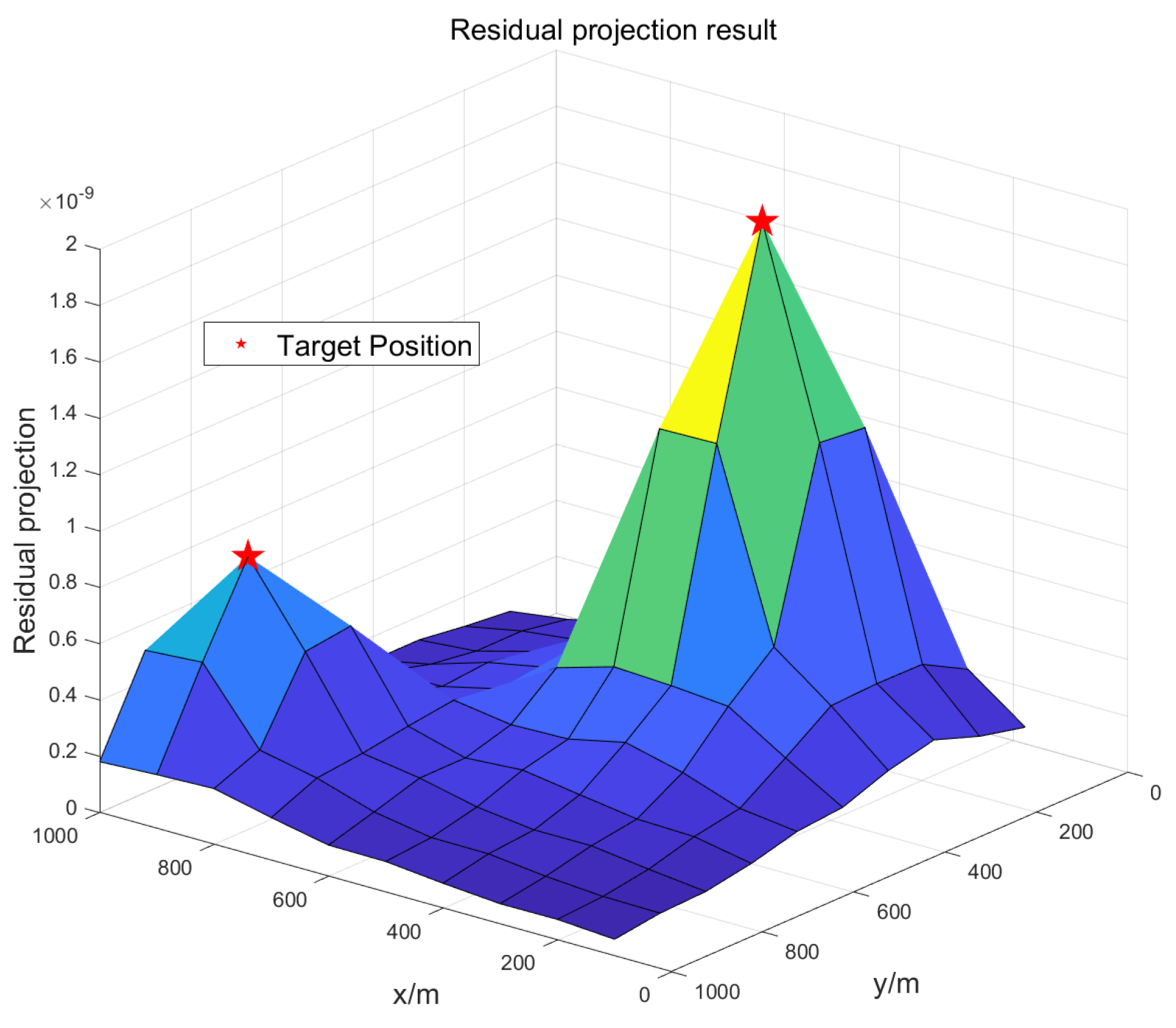
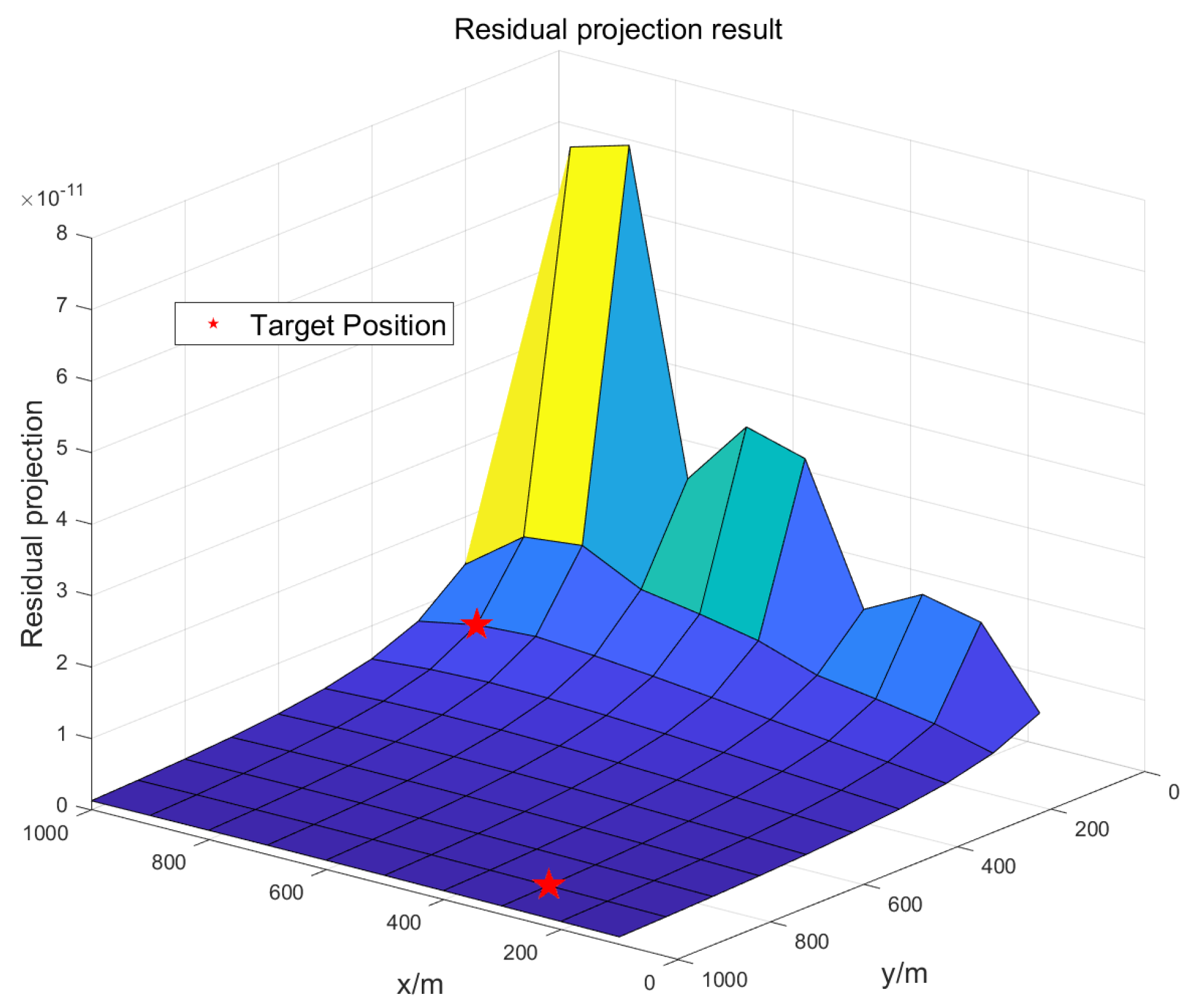
4.2. Simulation Result

Assuming a scenario with two signal sources and thirty mobile devices, Figure 3 shows the residual projection results of a classical sparse optimization algorithm, where the signal sources are encompassed within the mobile devices’ range. This is based on a compressed sensing algorithm that facilitates the estimation of the signal sources’ positions by acquiring the most compatible atoms. However, in this scenario, the signal sources are situated within the mobile devices’ surrounding area. In practical localization scenarios, signal sources are often positioned outside the mobile devices’ envelopment, necessitating the devices to locate distant signal sources.

Figure 4 shows the residual projection results of a classical sparse optimization algorithm when the signal source is located outside the envelopment of mobile devices. In scenarios involving long-distance localization, the residual projection fails to accurately highlight the target location information. This limitation arises because the signal source in this scenario is positioned behind the mobile devices, leading to the concentration of the peak regions of the residual projection near the edge closest to the mobile devices’ direction. Consequently, traditional sparse localization methods are ineffective for long-distance localization.

As depicted in Figure 5, the residual projection results in long-distance localization scenarios indicate that, under the block sparse model, the residual projection is globally influenced by the long-distance context, with projections near the direction of mobile devices being generally elevated. However, with the incorporation of the time-delay element in the model, it is evident from the residual projections that the block sparse model is capable of facilitating the localization of signal sources situated outside the envelopment of mobile devices.

To assess the impact of the mobile devices’ coverage status of the signal source on localization performance, it is assumed that the two regions gradually separate from an overlapping state, with the signal source region shifting to one side by a distance of $D=6\mathrm{km}$. The MCS and target signal source regions are both set as 4 km by 4 km square areas. Figure 6 shows the impact of mobile device coverage of signal sources on localization performance. As the signal source region progressively shifts to one side, the mobile devices transition from encompassing the signal sources to being situated on one side of them. The scenario is set with $K=3$ signal sources and $M=40$ mobile devices, with an $SNR$ of 15 dB. In this simulation, the impact on traditional sparse localization algorithms and block sparse localization algorithms is compared. Traditional sparse localization algorithms employ Orthogonal Matching Pursuit (OMP), Subspace Pursuit (SP), and Sparsity Adaptive Matching Pursuit (SAMP) algorithms. The OMP algorithm is a classical compressed sensing algorithm. The SP and SAMP algorithms, which introduce a subspace mechanism, exhibit a certain improvement in positioning performance over the OMP algorithm. As the distance of the signal source region’s shift increases, the accuracy of localization gradually decreases, dropping to zero when the two regions are completely separated. Block sparse localization algorithms employ the BOMP and UBRD methods. Even when the two regions are completely separated, block sparse algorithms experience a reduction in localization precision but still maintain a high probability of accurate localization.

Figure 7 shows the performance of different block sparse algorithms under various scenarios. In this simulation, the number of signal sources and mobile devices is the same as in the previous example, with the $SNR$ ranging from −15 dB to 15 dB. Two scenarios are presented in the simulation: source encirclement, where the mobile devices encompass the signal sources, and source isolation, where the signal sources are outside the mobile device enclosure. The threshold for the TBOMP algorithm is set at $\epsilon =2.5\times {10}^{-4}$, while the false alarm probability for the UBRD algorithm is set at $P_{fa}^{\tau }=0.04$. As shown, the localization performance of block sparse algorithms in the source isolation scenario is slightly reduced compared to the source encirclement scenario, yet still achieves an accuracy rate of over 0.95. Due to the known sparsity, the BOMP algorithm exhibits the highest accuracy, although sparsity is difficult to predetermine in real-world scenarios. The UBRD algorithm maintains commendable localization precision even in low-SNR conditions with unknown sparsity.

In practical scenarios, off-grid issues frequently arise, which can be equivalently characterized as situations involving a reduction in the number of sensors. Figure 8 shows the impact of the number of mobile devices on localization performance, set in a scenario with an $SNR$ of 15 and $K=3$ signal sources. As demonstrated in the figure, an increase in the number of mobile devices results in higher localization accuracy.

Figure 9 shows the impact of different scenarios on localization performance. In Figure 9a, the sensor node area is offset from the signal source area by D = 7000 m, and in Figure 9b, the offset is set to D = 8000 m. From the signal-to-noise ratio and positioning accuracy curves, it can be inferred that even in long-distance positioning scenarios at greater distances, the UBRD algorithm achieves commendable localization results, demonstrating robust adaptability to different environments. Figure 9c and Figure 9d, respectively, showcase the signal-to-noise ratio and positioning accuracy graphs for areas of size 500 m by 500 m and 2 km by 2 km. These figures illustrate that the UBRD algorithm maintains high positioning accuracy across different area sizes, verifying the algorithm’s precision in localization. In Figure 9e,f, the signal source frequencies are set to f = 100 MHz and f = 800 MHz, respectively. The results illustrate that the algorithm is capable of achieving commendable localization performance across a wide range of frequencies.

Figure 10 shows the localization accuracy across different algorithmic parameters, setting the threshold of the TBOMP algorithm at $\epsilon =2.5\times {10}^{-4}$ and $\epsilon =3\times {10}^{-4}$, and the false alarm probability of the UBRD algorithm at $P_{fa}^{\tau }=0.04$ and $P_{fa}^{\tau }=0.05$. The simulation results reveal that an increased threshold setting for the TBOMP algorithm improves localization accuracy under conditions of low SNR, yet diminishes accuracy under high SNR conditions. Similarly, setting a higher false alarm probability for the UBRD algorithm enhances localization accuracy under low SNR conditions, but reduces precision under high SNR conditions.

Figure 11 shows the accuracy of positioning in scenarios where the strength of the signal source is inconsistent. From Figure 11, the strength of the signal source, denoted as P, was configured to randomly fluctuate between 10 dB and 20 dB. The results from the simulation indicate that discrepancies in signal source strength lead to a decrease in positioning precision. However, accurate positioning can be achieved under conditions of higher signal-to-noise ratios.

5. Conclusions

This paper introduces a proposed unilateral branch ratio decision (UBRD) algorithm. The UBRD algorithm, grounded in block sparsity concepts, facilitates signal source localization. Leveraging a time–frequency domain composite block sparse model proposed in this study, the UBRD algorithm surpasses traditional sparse localization methods in achieving localization functionality in scenarios such as long-distance environments. By statistically deriving the branch residual ratio, an adaptive decision threshold for controlling the iterative process is obtained. Simulation results indicate that the UBRD algorithm, even in long-distance scenarios without prior information, attains a higher probability of accurate localization, demonstrating its broader adaptability across various contexts.

References

1. Capponi, A.; Fiandrino, C.; Kantarci, B.; Foschini, L.; Kliazovich, D.; Bouvry, P. A survey on mobile crowdsensing systems: Challenges, solutions, and opportunities. IEEE Commun. Surv. Tutor. 2019, 21, 2419–2465. [Google Scholar] [CrossRef]
2. Zhang, C.; Zhu, L.; Xu, C.; Liu, X.; Sharif, K. Reliable and privacy-preserving truth discovery for mobile crowdsensing systems. IEEE Trans. Dependable Secur. Comput. 2019, 3, 1245–1260. [Google Scholar] [CrossRef]
3. Zhang, C.; Zhao, M.; Zhu, L.; Wu, T.; Liu, X. Enabling efficient and strong privacy-preserving truth discovery in mobile crowdsensing. IEEE Trans. Dependable Secur. Comput. 2022, 17, 3569–3581. [Google Scholar] [CrossRef]
4. Friedlander, B. A passive localization algorithm and its accuracy analysis. IEEE J. Ocean. Eng. 1987, 1, 234–245. [Google Scholar] [CrossRef]
5. Zhang, W.; Yang, D.; Wu, W.; Peng, H.; Zhang, N.; Zhang, H.; Shen, X. Optimizing federated learning in distributed industrial IoT: A multi-agent approach. IEEE J. Sel. Areas Commun. 2021, 12, 3688–3703. [Google Scholar] [CrossRef]
6. Abualsaud, K.; Elfouly, T.M.; Khattab, T.; Yaacoub, E.; Ismail, L.S.; Ahmed, M.H.; Guizani, M. A survey on mobile crowd-sensing and its applications in the IoT era. IEEE Access 2018, 7, 3855–3881. [Google Scholar] [CrossRef]
7. Fawad, M.; Khan, M.Z.; Ullah, K.; Alasmary, H.; Shehzad, D.; Khan, B. Enhancing Localization Efficiency and Accuracy in Wireless Sensor Networks. Sensors 2023, 5, 2796. [Google Scholar] [CrossRef] [PubMed]
8. Viani, F.; Rocca, P.; Benedetti, M.; Oliveri, G.; Massa, A. Electromagnetic passive localization and tracking of moving targets in a WSN-infrastructured environment. Inverse Probl. 2010, 7, 074003. [Google Scholar] [CrossRef]
9. Guo, W.; Zhu, W.; Yu, Z.; Wang, J.; Guo, B. A survey of task allocation: Contrastive perspectives from wireless sensor networks and mobile crowdsensing. IEEE Access 2019, 7, 78406–78420. [Google Scholar] [CrossRef]
10. Amundson, I.; Koutsoukos, X.D. A survey on localization for mobile wireless sensor networks. In International Workshop on Mobile Entity Localization and Tracking in GPS-Less Environments; Springer: Berlin/Heidelberg, Germany, 2009; pp. 235–254. [Google Scholar]
11. Niculescu, D.; Nath, B. Ad hoc positioning system (APS). In GLOBECOM’01. IEEE Global Telecommunications Conference (Cat. No. 01CH37270); IEEE: Washington, DC, USA, 2001; Volume 5, pp. 2926–2931. [Google Scholar]
12. Patwari, N.; Hero, A.O.; Perkins, M.; Correal, N.S.; O’dea, R.J. Relative location estimation in wireless sensor networks. IEEE Trans. Signal. Proces. 2003, 8, 2137–2148. [Google Scholar] [CrossRef]
13. Vossiek, M.; Wiebking, L.; Gulden, P.; Wieghardt, J.; Hoffmann, C.; Heide, P. Wireless local positioning. IEEE Microw. Mag. 2003, 4, 77–86. [Google Scholar] [CrossRef]
14. Gui, L.; Val, T.; Wei, A.; Dalce, R. Improvement of range-free localization technology by a novel DV-hop protocol in wireless sensor networks. Ad Hoc Netw. 2015, 24, 55–73. [Google Scholar] [CrossRef]
15. Tomic, S.; Beko, M.; Dinis, R. RSS-based localization in wireless sensor networks using convex relaxation: Noncooperative and cooperative schemes. IEEE Trans. Veh. Technol. 2014, 5, 2037–2050. [Google Scholar] [CrossRef]
16. Wang, Y.; Ho, K.C. An asymptotically efficient estimator in closed-form for 3-D AOA localization using a sensor network. IEEE Trans. Wirel. Commun. 2015, 12, 6524–6535. [Google Scholar] [CrossRef]
17. Pak, J.M.; Ahn, C.K.; Shi, P.; Shmaliy, Y.S.; Lim, M.T. Distributed hybrid particle/FIR filtering for mitigating NLOS effects in TOA-based localization using wireless sensor networks. IEEE Trans. Ind. Electron. 2016, 6, 5182–5191. [Google Scholar]
18. Gholami, M.R.; Gezici, S.; Strom, E.G. TDOA based positioning in the presence of unknown clock skew. IEEE Trans. Commun. 2013, 6, 2522–2534. [Google Scholar] [CrossRef]
19. Dai, L.; Wang, B.; Yuan, Y.; Han, S.; Chih-Lin, I.; Wang, Z. Non-orthogonal multiple access for 5G: Solutions, challenges, opportunities, and future research trends. IEEE Commun. Mag. 2015, 9, 74–81. [Google Scholar] [CrossRef]
20. Moreno-Salinas, D.; Pascoal, A.M.; Aranda, J. Optimal sensor placement for multiple target positioning with range-only measurements in two-dimensional scenarios. Sensors 2013, 8, 10674–10710. [Google Scholar] [CrossRef] [PubMed]
21. Xu, S.; Wu, L.; Doğançay, K.; Alaee-Kerahroodi, M. A hybrid approach to optimal TOA-sensor placement with fixed shared sensors for simultaneous multi-target localization. IEEE Trans. Signal Process. 2022, 70, 1197–1212. [Google Scholar] [CrossRef]
22. Candès, E.J.; Wakin, M.B. An introduction to compressive sampling. IEEE Signal. Process. Mag. 2008, 2, 21–30. [Google Scholar] [CrossRef]
23. Cevher, V.; Duarte, M.F.; Baraniuk, R.G. Distributed target localization via spatial sparsity. In Proceedings of the 2008 16th European Signal Processing Conference, Lausanne, Switzerland, 25–29 August 2008; IEEE: Washington, DC, USA, 2008; pp. 1–5. [Google Scholar]
24. Feng, C.; Valaee, S.; Tan, Z. Multiple target localization using compressive sensing. In Proceedings of the GLOBECOM 2009–2009 IEEE Global Telecommunications Conference, Honolulu, HI, USA, 4 March 2010; IEEE: Washington, DC, USA, 2009; pp. 1–6. [Google Scholar]
25. Zhang, B.; Cheng, X.; Zhang, N.; Cui, Y.; Li, Y.; Liang, Q. Sparse target counting and localization in sensor networks based on compressive sensing. In Proceedings of the 2011 Proceedings IEEE INFOCOM, Shanghai, China, 10–15 April 2011; IEEE: Washington, DC, USA, 2011; pp. 2255–2263. [Google Scholar]
26. Feng, C.; Au, W.S.A.; Valaee, S.; Tan, Z. Received-signal-strength-based indoor positioning using compressive sensing. IEEE Trans. Mob. Comput. 2011, 12, 1983–1993. [Google Scholar] [CrossRef]
27. Qi, P.; Li, Z.; Li, H.; Xiong, T. Blind sub-Nyquist spectrum sensing with modulated wideband converter. IEEE Trans. Veh. Technol. 2018, 5, 4278–4288. [Google Scholar] [CrossRef]
28. Baraniuk, R.G.; Cevher, V.; Duarte, M.F.; Hegde, C. Model-based compressive sensing. IEEE Trans. Inf. Theory 2010, 4, 1982–2001. [Google Scholar] [CrossRef]
29. Zhang, X.; Xu, W.; Cui, Y.; Lu, L.; Lin, J. On recovery of block sparse signals via block compressive sampling matching pursuit. IEEE Access 2019, 7, 175554–175563. [Google Scholar] [CrossRef]
30. Hinkley, D.V. On the ratio of two correlated normal random variables. Biometrika 1969, 3, 635–639. [Google Scholar] [CrossRef]
Figure 1. MCS sparse localization scene.
Electronics 13 01024 g001
Figure 2. Flowchart of the UBRD algorithm.
Electronics 13 01024 g002
Figure 3. The residual projection result of signal sources within the vicinity surrounded by mobile devices.
Electronics 13 01024 g003
Figure 4. The residual projection result of the signal source situated outside the enclosure formed by mobile devices.
Electronics 13 01024 g004
Figure 5. Residual projection result for block sparse localization in long-range localization scenarios.
Electronics 13 01024 g005
Figure 6. The impact of mobile device coverage of signal sources on localization performance.
Electronics 13 01024 g006
Figure 7. The performance of different block sparse algorithms in various scenarios.
Electronics 13 01024 g007
Figure 8. The impact of the number of mobile devices on localization performance.
Electronics 13 01024 g008
Figure 9. Impact of different scenarios on localization performance. (a) SNR and positioning accuracy graph at D = 7000 m. (b) SNR and positioning accuracy graph at D = 8000 m. (c) SNR and positioning accuracy graph in a 500 m × 500 m area. (d) SNR and positioning accuracy graph in a 2 km × 2 km area. (e) SNR and positioning accuracy graph at f = 100 MHz. (f) SNR and positioning accuracy graph at f = 800 MHz.
Electronics 13 01024 g009
Figure 10. Localization accuracy under different algorithmic parameters.
Electronics 13 01024 g010
Figure 11. Localization accuracy in scenarios with inconsistent signal source intensity.
Electronics 13 01024 g011
Disclaimer/Publisher’s Note: The statements, opinions and data contained in all publications are solely those of the individual author(s) and contributor(s) and not of MDPI and/or the editor(s). MDPI and/or the editor(s) disclaim responsibility for any injury to people or property resulting from any ideas, methods, instructions or products referred to in the content.