Reducing the Length of Dynamic and Relevant Slices by Pruning Boolean Expressions

Abstract

Dynamic and relevant (backward) slicing helps programmers in the debugging process by reducing the number of statements in an execution trace. In this paper, we propose an approach called pruned slicing, which can further reduce the size of slices by reasoning over Boolean expressions. It adds only those parts of a Boolean expression that are responsible for the evaluation outcome of the Boolean expression to the set of relevant variables. We empirically evaluate our approach and compare it to dynamic and relevant slicing using three small benchmarks: the traffic collision avoidance system (TCAS), the Refactory dataset, and QuixBugs. Pruned slicing reduces the size of the TCAS slices on average by 10.2%, but it does not reduce the slice sizes of the Refactory and QuixBugs programs. The times required for computing pruned dynamic and relevant slices are comparable to the computation times of non-pruned dynamic and relevant slices. Thus, pruned slicing is an extension of dynamic and relevant slicing that can reduce the size of slices while having a negligible computational overhead.

1. Introduction

Backward slicing is a source code analysis technique that identifies all statements that contribute to the value of a certain variable at a point of interest [1]. Since slicing reduces the number of statements, it is particularly useful in fault localization [2]. Software developers spend half of their total work time on testing and debugging [3]. On average, a programmer needs 3.0 h to reproduce a bug, 4.4 h to localize the faulty line(s), and 2.1 h to write a fix [4]. Therefore, decreasing the time required to localize a bug decreases the total debugging time and saves resources and money.

The smaller a slice is, the easier it is for a programmer to locate the faulty source code line(s). Dynamic slices [5] contain those statements that influence the value of a certain variable for a particular execution of the program. They compute the same result as the original program for the variable of interest, but they are usually smaller than their static counterparts. Since developers often reproduce a bug before they begin with the fault-localization process, the input for the execution of the program is usually available, and therefore dynamic slicing can be used instead of static slicing.

One problem with dynamic slicing when used for fault localization is that the actually faulty code line(s) may not be part of the slice. This happens when the fault results in the non-execution of a loop or branch of a conditional statement. Relevant slicing solves this problem by adding such statements to the slice [6]. Therefore, relevant slices can be larger than dynamic slices.

In this paper, we present pruned slicing, a technique that reduces the size of dynamic and relevant slices by reasoning over Boolean expressions. Pruned slicing adds only those parts of Boolean expressions to the slice that actually contribute to the outcome of the Boolean expressions. While all of the Boolean sub-expressions might be evaluated, not all of them might contribute to the result. For example, the expression ‘a and b and c’, where a = true, b = true, and c = false, evaluates to false; the outcome of this expression can only be changed when the value of c is changed. Therefore, all statements that change c should be part of the slice, but the statements that change a and b need not be part of the slice.

To motivate our approach, we use the code snippet illustrated in Algorithm 1. This code snippet [7] is taken from Pandas, a well-known data analysis library for Python. For the sake of clarity, we have only indicated those source code lines that are necessary to convey our idea. The line numbers indicated in the figure mirror the line numbers from the source code file as in the commit. Assume that a programmer has reproduced a bug. He notices that tail has the wrong value after executing line 943 and computes the dynamic slice for tail. Among other statements, this slice contains lines 883, 885, and 894. When manually investigating the slice and the variables’ values, the programmer realizes that the condition in line 938 evaluated to true because the second part of the condition (i.e., not (len(’, ’.join(head)) < display_width and ...)) evaluated to true; the first part (i.e., is_truncated) evaluated to false and therefore did not contribute to the decision that the then-branch should be taken. Therefore, the programmer knows that is_truncated cannot be responsible for the observed bug, and he can focus on the other parts of the slice. Pruned slicing relieves the programmer from this manual reasoning effort for conditionals; it adds only those parts of nested Boolean expressions to the slice that actually contribute to the result of the expression. In this example, the pruned slice does not contain lines 883, 885, and 894.

Algorithm 1 Expert analysis of the file base.py from the Python library Pandas.

868 def _format_data(self, name=None): … 883   n = len(self) 884   sep = ’,’ 885   max_seq_items = get_option(’display.max_seq_items’) or n … 894   is_truncated = n > max_seq_items … 938   if (is_truncated or 939      not (len(’,⎵’.join(head)) < display_width and 940        len(’,⎵’.join(tail)) < display_width)): 941     max_len = max(best_len(head), best_len(tail)) 942     head = [x.rjust(max_len) for x in head] 943     tail = [x.rjust(max_len) for x in tail]

The reasoning over Boolean expressions is closely related to short-circuit evaluation. In short-circuit evaluations, the second term of a binary Boolean expression is only evaluated if the result of the first term is not sufficient to determine the final result of the Boolean expression. While short-circuit evaluation has been discussed in the context of static slicing [8], to the best of our knowledge, it has not yet been discussed in the context of dynamic slicing in the scientific literature. For this reason, we will discuss short-circuit evaluations for dynamic slicing in Section 3.

In this paper, we will empirically compare the slice length of dynamic slices, relevant slices, pruned dynamic slices, and pruned relevant slices based on small Python 3 programs from three different benchmarks, namely QuixBugs [9], the Refactory dataset [10], and a Python 3 implementation of TCAS [11]. The results of this evaluation are quite different for the three benchmarks. While relevant slicing has no impact on the TCAS programs, it increases the slice size for 34% of the Refactory programs and 12% of the QuixBugs programs. Pruned slicing reduces the size of 76% of the TCAS slices, only two slices from the Refactory set, and none of the slices of the QuixBugs programs. In the empirical evaluation (see Section 7), we will discuss the reasons for these results.

The main contributions of this paper are as follows:

• A discussion of short-circuit evaluation for dynamic slicing.
• The introduction of pruned slicing.
• A proof-of-concept implementation of a dynamic, relevant, and pruned slicer for Python 3 programs.
• An empirical evaluation of dynamic and relevant slicing with short-circuit evaluation and pruned slicing on three small benchmarks.

This paper is based on our previous work on pruned slicing presented at the International Working Conference on Source Code Analysis and Manipulation (SCAM) [12]. It improves our previous work by providing the following contributions:

• We extend our evaluation to relevant slicing and pruned relevant slicing. In particular, we compare dynamic and relevant slicing with respect to executability, correct results, slice length, and computation time.
• We extend our prototype slicer by implementing a relevant slicer.

The remainder of this article is structured as follows. We discuss the related works with respect to existing slicing approaches, challenges for building a slicer, and fields of application in Section 2. In Section 3, we discuss the syntax of Boolean expressions and explain dynamic and relevant slicing, as well as dynamic slicing with short-circuit evaluation. In Section 4, we explain how pruned slicing works. In Section 5, we discuss the relation of the different slice types. Section 6 introduces the technical details of our prototype implementation and explains how we tested the implementation utilizing metamorphic testing. Furthermore, we list the limitations of this prototype and discuss the steps necessary to build a real-world dynamic slicer for Python. We evaluate the basic dynamic and relevant slicer, as well as our pruned slicing extension, in Section 7, and we conclude this paper in Section 8.

2. Related Works

Slicing dates back to the 1980s when Mark Weiser [1] introduced static (backward) slicing. A static slice contains all statements that contribute to the computation of a specific variable’s value. A static slice computes the same result for this variable as the original program when it is executed on the same input as the original program.

Bergeretti and Carré [13] introduced the concept of forward slicing. A forward slice computes all parts of a program that will be influenced by changing a specific statement.

Later on, Korel and Laski [5] introduced the concept of dynamic slicing. A dynamic backward slice contains all statements that contribute to the computation of a specific variable’s value for a certain input. In contrast to its static counterpart, dynamic slicing must not compute the same result for an arbitrary input but only for the predefined input. It does only contain statements that were actually executed.

A weakness of dynamic slicing is that the slice does not contain those statements that could have affected the value of the variable of interest if they had been evaluated differently. In particular, when using dynamic slicing for fault-localization purposes, important statements might be missing in the dynamic slice. Relevant slicing fixes this problem by considering the potential relevant variables [6].

However, relevant slicing fails to include statements that modify a wrong memory location. To solve this problem, Li and Orso [14] developed PMD-Slicer, a dynamic slicer that takes into consideration potential memory-address dependencies.

An approximate dynamic slice [15] is the intersection of the execution trace and the static slice. The approximate dynamic slice is a superset of the relevant slice.

Many other slicing techniques have been developed. We refer the interested reader to Tip’s survey [16] and Silva’s comparison of slicing techniques [17] for more information on the purpose and application areas of the different slicing techniques and to Wong et al.’s survey on software fault localization [18].

There exist several research prototype implementations of slicers. In his Bachelor’s thesis, Hammacher [19] developed JavaSlicer, a dynamic backward slicer for Java. Unfortunately, this slicer only supports JDK versions 1.6 and 1.7. Ahmed et al. developed Slicer4J [20], a dynamic slicer for programs written in Java 9 (or below). The same authors developed Mandoline [21], a dynamic slicer for Android applications. Galindo et al. [22,23] developed Java SDG Slicer, a static slicer that is based on the system dependence graph (SDG). Nguyen et al. [24] proposed WebSlice, which generates program slices across several programming languages, e.g., PHP, JavaScript, and SQL. Recently, Stiévenart et al. [25] proposed an approach to slice WebAssembly programs.

Developing a slicer that supports the whole range of functionality of today’s programming languages is challenging, particularly the handling of exception-related constructs [26], unconditional jumps [27], object orientation [27], concurrency [28], and shared memory [29]. The aforementioned papers highlight that there are still many issues that need to be addressed to develop slicers for programs written in modern programming languages.

Despite the massive effort required to build a real-world slicer, slicing is useful in many areas. In particular, fault localization benefits from backward slicing approaches because slicing can be used in combination with other fault-localization techniques. Gosh and Singh [30] combined dynamic slicing with spectrum-based fault localization (SBFL). Soremekun et al. [31] empirically evaluated the effectiveness of slicing and SBFL. They recommend a hybrid approach for fault localization: a programmer should first examine the five highest-ranked statements from SBFL; if the fault is not detected within these five statements, the programmer should examine the dynamic slice. Recently, Soha et al. [2] proposed the use of slice-based spectra instead of coverage-based spectra in SBFL.

Besides fault localization, slicing can be also used in other endeavors, for example, for test case separation [32], deobfuscating strings in mobile applications [33], detecting security patches [34], and detecting API misuses [35].

3. Background

First, we discuss the structure of Boolean expressions in Section 3.1. Then, we discuss dynamic slicing (Section 3.2), short-circuit evaluation (Section 3.3), and relevant slicing (Section 3.4).

3.1. Syntax of Boolean Expressions

Definition 1.

A Boolean expression e is recursively defined as follows:

• $e_1\mathit{AND}{e}_2$, where $e_1$ and $e_2$ are Boolean expressions;
• $e_1\mathit{OR}{e}_2$, where $e_1$ and $e_2$ are Boolean expressions;
• $\mathit{NOT}{e}_1$, where $e_1$ is a Boolean expression;
• $\mathit{True}$;
• $\mathit{False}$;
• Any expression that evaluates/casts to a Boolean value, e.g., ‘3 < 5’, ‘0’, ‘None’;
• A function/method call that returns a value interpretable as a Boolean.

We define the function eval(e) that returns the evaluation outcome of a Boolean expression e, i.e., true or false.

In Python, many expressions dynamically cast to a Boolean value depending on their context. For example, empty lists, sets, and dictionaries are interpreted as false, and their non-empty counterparts are interpreted as true when used as conditionals or as part of a Boolean expression. Similarly, empty strings are interpreted as false, and non-empty strings are interpreted as true. ‘0’ is interpreted as false, and any other integer value is interpreted as true. None evaluates to false. This list is for illustration purposes and is by no means complete.

3.2. Dynamic Slicing

We adapt Korel and Laski’s definition of dynamic slicing [5]. First, we formally define the execution trace and the slicing criterion. Then, we explain an algorithm for computing small dynamic slices.

The execution trace $\tau$ results from the execution of program $\mathrm{\Pi }$ on input $\omega$.

Definition 2.

An execution trace τ is the finite sequence of instructions $\langle n_1,\cdots ,n_q\rangle$ that was executed when calling $\mathrm{\Pi }\left(\omega \right)$. In case the program does not terminate, τ is a finite sequence up to a threshold. Each instruction $n_i$ consists of the following:

• Instruction number X and execution number i: The instruction number X is the line number of the statement in the source code, and the execution number i is the position of the statement in the execution trace, i.e., $X^i$ means that statement X is the ith statement in the execution trace.
• Instruction type $T\left(X^i\right)$: The instruction type is either control (C) or assignment (A). Source code often comprises other types of statements (e.g., print(x)), but for the sake of simplicity, we restrict ourselves to these types.
• Set of referenced (or used) variables $U\left(X^i\right)$: $U\left(X^i\right)$ comprises all variables that are referenced in statement $X^i$. For example, for statement $X^i$:a[i]=b, the used variables are $U\left(X^i\right)=\{i,b\}$. For function/method calls/definitions, $U\left(X^i\right)$ is a variable vector to allow the matching of parameters.
• Set of defined variables $D\left(X^i\right)$: $D\left(X^i\right)$ comprises all variables whose values are changed in statement $X^i$. For example, for statement $X^i$:a[i]=b, the set of defined variables is $D\left(X^i\right)=\left\{a\right\}$. For function/method calls/definitions, $D\left(X^i\right)$ is a variable vector to allow the matching of parameters.
• Set of control dependencies $C\left(X^i\right)$: A statement $X^i$ is control-dependent on another statement $Y^j$ (i.e., $Y^j\in C\left(X^i\right)$) if $X^i$ is only executed when $Y^j$ evaluates in a way that allows its execution, i.e., all statements in a loop body are control-dependent on the statement in the loop head, and all statements in the then and else branches are control-dependent on the if statement.

Example 1.

For demonstration purposes, we use the following code snippet as program Π in our running example:

1

a = x

2

b = y

3

c = z

4

d = y

5

if a < b or a < c or d < c:

6

  c = a

7

if b > c:

8

  c = b

9

d = c

Furthermore, we use $\omega =\{x=3,y=2,z=4\}$ as input. The execution trace τ for $\mathrm{\Pi }\left(\omega \right)$ is $\langle 1^1,2^2,3^3,4^4,5^5,6^6,7^7,9^8\rangle$, with the types, definitions, uses, and control dependencies shown in

Table 1. Instruction numbers X and execution numbers i, types $T\left(X^i\right)$ (A = assignment, C = control), definitions $D\left(X^i\right)$, uses $U\left(X^i\right)$, and control dependencies $C\left(X^i\right)$ for all instructions in $\tau$ of Example 1.

Xi	T (Xi)	D (Xi)	U (Xi)	C (Xi)
$1^1$	A	{a}	{x}	{ }
$2^2$	A	{b}	{y}	{ }
$3^3$	A	{c}	{z}	{ }
$4^4$	A	{d}	{y}	{ }
$5^5$	C	{ }	{a, b, c, d}	{ }
$6^6$	A	{c}	{a}	{5}
$7^7$	C	{ }	{b, c}	{ }
$9^8$	A	{d}	{c}	{ }

.

The slicing criterion consists of three parts: a program input $\omega$, an instruction/execution number $X^q$, and a variable name v.

Definition 3.

For an execution trace τ for a program Π that is executed with input ω, the triple $(\omega ,X^q,v)$ is a slicing criterion for variable name v if instruction/execution number $X^q\in \tau$.

Example 2.

The last definition of variable d is in line $9^8$. Therefore, $(\omega =\{x=3,y=2,z=4\},9^8,d)$ is a slicing criterion for program Π.

A dynamic slice behaves the same as the original program for the variable of interest for the given input.

Definition 4.

Any subset of statements ${\mathrm{\Pi }}^{\prime }\subseteq \mathrm{\Pi }$ is a valid dynamic slice for the slicing criterion $(\omega ,X^q,v)$ if and only if ${\mathrm{\Pi }}^{\prime }\left(\omega \right)$ is an executable program and computes the same final value for variable v as $\mathrm{\Pi }\left(\omega \right)$.

According to Definition 4, the original program as well as the set of executed statements are valid dynamic slices. However, we are interested in computing smaller slices. Since there exists no algorithm for finding state-minimal slices for arbitrary programs [1], we use an algorithm that computes small, but not necessarily minimal, dynamic slices (see Algorithm 2).

Algorithm 2: Simplified dynamic slicing algorithm.

1: procedure DynamicSlice($\tau ,(\omega ,X^q,v)$) 2:   $\mathit{slice}\leftarrow \left\{\right\}$ 3:   $\mathit{i}\leftarrow q$ 4:   $\mathit{relevant}\leftarrow v$ 5:   while $\mathit{i}>0$ do 6:     if $\mathit{relevant}\cap D\left(X^i\right)\ne \left\{\right\}$ then 7:       $C_{\mathit{new}}\leftarrow C\left(X^i\right)\setminus \mathit{slice}$ 8:       $\mathit{slice}\leftarrow \mathit{slice}\cup \left\{X\right\}\cup C_{\mathit{new}}$ 9:       $\mathit{relevant}\leftarrow (\mathit{relevant}\setminus D\left(X^i\right))\cup U\left(X^i\right)\cup U\left(C\left(X^i\right)\right)$ 10:       if $C_{\mathit{new}}\ne \left\{\right\}$ then 11:         $i\leftarrow \mathtt{maxExecutionNumberOfControlStatement}(\tau ,C_{\mathit{new}})$ 12:         continue 13:       end if 14:     end if 15:     $i\leftarrow i-1$ 16:   end while 17:   return $\mathit{slice}$ 18: end procedure

The algorithm traverses the execution trace $\tau$ in a backward direction (see lines 3, 5, and 15) and thereby keeps track of the relevant variables. The set of relevant variables is initialized with the variable indicated in the slicing criterion (line 4). Whenever a variable in the relevant variables is defined (line 6), the line and its control dependencies are added to the slice (line 8), and the relevant variables are updated (line 9).

To include the statements that change the values of variables used in the condition of loops even when the loop body is executed only once, we keep track of the newly added control statements (line 7). Whenever we add new control statements to the slice (line 10), we set i to the highest execution number of this control statement (line 11). Korel and Laski [5] used the Identity Relation to solve the problem caused by loops that are executed only once.

This algorithm terminates because the execution trace $\tau$ is finite according to Definition 2 and i is decremented in every loop iteration (line 15), except when new control flow statements are added (lines 10–13). The latter scenario is limited to the number of different control statements in the (finite) execution trace: once a control statement has been added to the slice, the control statement cannot be part of $C_{\mathit{new}}$ in a later iteration (see line 7). Since the execution trace is finite, the number of different control statements is also finite. Therefore, the algorithm terminates.

The algorithm illustrated in Algorithm 2 is a simplified version of the algorithm we actually implemented. While proper handling of language constructs, such as function calls and control flow statements for loops (e.g., break and continue), is essential for a slicer, they are not relevant in the context of this paper. For the sake of clarity, we therefore do not explain their handling here, but we provide the source code of our proof-of-concept prototype implementation for interested readers (see Section 8).

Example 3.

The algorithm in Algorithm 2 computes $\{1,2,3,4,5,6,9\}$ as the slice for the slicing criterion $(\omega =\{x=3,y=2,z=4\},9^8,d)$.

3.3. Short-Circuit Evaluation

While the slice $\{1,2,3,4,5,6,9\}$ in Example 3 is shorter than the complete program, it contains statements that are not required to fulfill Definition 4. In this section, we explain how slices can be further reduced using short-circuit evaluation.

In programming languages supporting short-circuit evaluation, the second part of a binary Boolean expression is only evaluated if the first part is not sufficient to determine the outcome of the expression. To consider short-circuit evaluations in dynamic slicing, we first have to define the set of effective uses $\overline{U}$: $\overline{U}\left(X^i\right)$ contains all variables that were referenced in statement X and actually evaluated in $X^i$. For example, for the assignment ‘a = b and c’ with eval(b) = false and eval(c) = true, the set of used variables U is $\{b,c\}$, whereas the set of effective uses $\overline{U}$ is $\left\{b\right\}$ because the second part of the expression is never evaluated.

Definition 5.

The set of effective uses $\overline{U}$ of an expression $\mathit{e}$ is as follows:

e	eval(${\mathit{e}}_1$)	eval(${\mathit{e}}_2$)	$\overline{U}\left(\mathit{e}\right)$
$e_1\mathit{AND}{e}_2$	true	?	$\overline{U}\left({\mathit{e}}_1\right)\cup \overline{U}\left({\mathit{e}}_2\right)$
	false	?	$\overline{U}\left({\mathit{e}}_1\right)$
$e_1\mathit{OR}{e}_2$	true	?	$\overline{U}\left({\mathit{e}}_1\right)$
	false	?	$\overline{U}\left({\mathit{e}}_1\right)\cup \overline{U}\left({\mathit{e}}_2\right)$
$\mathit{NOT}{e}_1$	?	-	$\overline{U}\left({\mathit{e}}_1\right)$
True	-	-	$\left\{\right\}$
False	-	-	$\left\{\right\}$
other	-	-	$U\left(\mathit{e}\right)$

The effective uses $\overline{U}\left(\mathit{e}\right)$ replace the sets of used variables $U\left(\mathit{e}\right)$ in line 9 of the dynamic slicing algorithm in Algorithm 2, i.e., $\mathit{relevant}\leftarrow (\mathit{relevant}\setminus D\left(X^i\right))\cup \overline{U}\left(X^i\right)\cup \overline{U}\left(C\left(X^i\right)\right)$.

Example 4.

In our running example, the first term of the condition in statement $5^5$ (i.e., $a<b$) evaluates to false and the second term ($a<c$) evaluates to true. Therefore, the third term ($d<c$) will not be evaluated, and the set of effective uses is therefore $\overline{U}\left(5^5\right)=\{a,b,c\}$. The short-circuit dynamic slice for the slicing criterion $(\omega =\{x=3,y=2,z=4\},9^8,d)$ is $\{1,2,3,5,6,9\}$.

To the best of our knowledge, short-circuit evaluation has not been discussed in the context of dynamic slicing. For this reason, in our SCAM paper [12], we investigated how the publicly available slicers Slicer4J [20] and JavaSlicer [19] handle short-circuit evaluations. We evaluated slicers for Java programs because, to the best of our knowledge, there currently exist no other slicers for Python programs.

We used a jar file containing the class illustrated in Figure 1 and the following test cases:

• Base test case $t_1:\{input=31,{\mathit{slice}}_{\mathit{exp}}=\{3,4,\left(5\right),6,7,\left(11\right)\}\}$, where both sub-expressions of line 6 ($a>2$ and $b<2$) evaluate to true.
• Base test case $t_2:\{input=33,{\mathit{slice}}_{\mathit{exp}}=\{3,4,\left(5\right),6,\left(8\right),9,\left(11\right)\}\}$, where the second sub-expression evaluates to false.
• Short-circuit test case $t_3:\{input=11,{\mathit{slice}}_{\mathit{exp}}=\{3,\left(5\right),6,\left(8\right),9,\left(11\right)\}\}$, where the first expression evaluates to false and thus the second expression is not evaluated.

Line numbers 5, 8, and 11 are in parentheses because of insufficient and ambiguous definitions of dynamic slicing. Although lines 5 and 8 are not part of the slice according to the Algorithm presented in Algorithm 2, they have to be part of the slices in order to generate executable code (see Definition 4). Line 11 does not change any variables of interest, but one could argue that programmers are also interested in seeing the lines they have indicated as slicing criteria in the slice.

Analogously, we created another jar file that contains the same class, but the statement in line 6 is changed to if(a>2 || b<2) to test the behavior where two expressions are connected with a logical or. For this example, we created three additional test cases ($t_4$, $t_5$, and $t_6$) to evaluate both the base behavior and the behavior in the case of short-circuit evaluation.

JavaSlicer computes the correct slices for all test cases. Slicer4J computes the correct slices for $t_1$, $t_2$, $t_4$, and $t_5$, but the computed slices for $t_3$ and $t_6$ are too small as they do not contain lines 3 and 6. This is particularly problematic when using slicing for debugging purposes, as a potentially faulty statement might be missing. We refer the interested reader to our SCAM paper [12] for more information about this experiment.

Short-circuit evaluation not only helps make slices shorter but also avoids the problem of adding code to the slice that should not be executed. A common usage of short-circuit evaluation is to check whether an object exists before checking the value of one of its member variables, e.g., if obj is not None and obj.getValue() > 0. The code obj.getValue() should only be called when the object exists. Because of such scenarios, it is essential that short-circuit evaluation is properly implemented in dynamic slicing.

3.4. Relevant Slicing

The problem with dynamic slicing in the context of fault localization is that the slice might not contain the statement(s) that have actually caused the fault. This happens when a fault changes the value of a variable used in the condition of a loop or conditional in such a way that the condition evaluates to false instead of true, and the loop body or the conditional branch that would have changed a relevant variable is not executed.

Besides the issue that the actually faulty statement(s) might be missing in the slice, dynamic slicing causes another problem: under certain circumstances, the sliced program might not behave as the original program because of an incomplete dynamic slice as the following example demonstrates.

Example 5.

We use the following code snippet from the Refactory dataset (question 3, correct_3_056.py) [10] asΠand compute the dynamic slice for $(\omega =\{\mathit{lst}=[3,3]\},{10}^{15},l)$.

1

def remove_extras(lst):

2

  l=[]

3

  for i in lst:

4

    checker=True

5

    for k in l:

6

      if k==i:

7

        checker=False

8

    if checker:

9

      l+=[i]

10

  return l

The execution trace is $\tau =\langle 1^1,2^2,3^3,4^4,5^5,8^6,9^7,3^8,4^9,5^{10},6^{11},7^{12},8^{13},3^{14},{10}^{15}\rangle$, and the dynamic slice is $\{1,2,3,4,8,9,10\}$. The slice does not contain statements 5, 6, and 7 because they are not necessary according to the dynamic slicing algorithm. However, the slice computes a different result for ω than the original program, i.e., $\mathrm{\Pi }\left(\omega \right)=\left[3\right],$ ${\mathrm{\Pi }}_{\mathit{dyn}\_\mathit{slice}}\left(\omega \right)=[3,3]$.

To solve this problem, the statements that did not affect the relevant variables but would have affected them if they had been evaluated differently have to be considered [6]. Therefore, we extend our execution trace $\tau =\langle n_1,\cdots ,n_q\rangle$ with static information from the source code. Each instruction $n_i$ is assigned an additional attribute, namely the set of potential relevant variables $P\left(X^i\right)$.

Definition 6.

The set of potential relevant variables $P\left(X^i\right)$ is as follows:

• The set of variables that could be (re)defined in any of the branches of the conditional in case of conditionals.
• The set of variables that would be (re)defined in the loop body in case of loops.
• $\left\{\right\}$ for assignments (i.e., $T\left(X^i\right)=A$).

Example 6.

The sets of potential relevant variables P for Example 5 are as follows: For assignments, P is always the empty set, i.e., $P\left(2^2\right)=P\left(4^4\right)=P\left(9^7\right)=P\left(4^9\right)=P\left(7^{12}\right)=P\left({10}^{15}\right)=\left\{\right\}$. For the loops and the conditionals, P is $P\left(3^3\right)=P\left(3^8\right)=P\left(3^{14}\right)=\{\mathit{checker},\mathit{l}\}$, $P\left(5^5\right)=P\left(5^{10}\right)=\left\{\mathit{checker}\right\}$, $P\left(6^{11}\right)=\left\{checker\right\}$, and $P\left(8^6\right)=P\left(8^{13}\right)=\left\{l\right\}$.

Algorithm 3 highlights the changes necessary to transform the dynamic slicing algorithm into a relevant slicing algorithm. Essentially, we have to additionally check for all control statements if the set of potential relevant variables contains variables of interest, i.e., relevant variables (line 15). If this is the case, we add the control statement to the slice (line 16). The variables that are referenced in the control statement are added to the set of relevant variables in line 17.

Algorithm 3: Relevant Slicing algorithm: Changes necessary for short-circuit evaluation are highlighted in blue; changes necessary for relevant slicing are highlighted in red.

1: procedureRelevantSlice($\tau ,(\omega ,X^q,v)$) 2:   $\mathit{slice}\leftarrow \left\{\right\}$ 3:   $\mathit{i}\leftarrow q$ 4:   $\mathit{relevant}\leftarrow v$ 5:   while $\mathit{i}>0$ do 6:     if $\mathit{relevant}\cap D\left(X^i\right)\ne \left\{\right\}$ then 7:       $C_{\mathit{new}}\leftarrow C\left(X^i\right)\setminus \mathit{slice}$ 8:       $\mathit{slice}\leftarrow \mathit{slice}\cup \left\{X\right\}\cup C_{\mathit{new}}$ 9:       $\mathit{relevant}\leftarrow (\mathit{relevant}\setminus D\left(X^i\right))\cup \overline{U}\left(X^i\right)\cup \overline{U}\left(C\left(X^i\right)\right)$ 10:       if $C_{\mathit{new}}\ne \left\{\right\}$ then 11:         $i\leftarrow \mathtt{maxExecutionNumber}(\tau ,C_{\mathit{new}})$ 12:         continue 13:       end if 14:     end if 15:     if  $T\left(X^i\right)==C\wedge \mathit{relevant}\cap P\left(X^i\right)\ne \left\{\right\}$ then 16:       $\mathit{slice}\leftarrow \mathit{slice}\cup \left\{X\right\}$ 17:       $\mathit{relevant}\leftarrow \mathit{relevant}\cup \overline{U}\left(X^i\right)$ 18:     end if 19:     $i\leftarrow i-1$ 20:   end while 21:   return $\mathit{slice}$ 22: end procedure

Example 7.

The relevant slice for Example 5 is $\{1,2,3,4,5,6,7,8,9,10\}$. In contrast to the dynamic slice, it contains statements 5, 6, and 7 because when analyzing $8^{13}$, $T\left(X^i\right)==C\wedge \mathit{relevant}\cap P\left(X^i\right)\ne \left\{\right\}$, and therefore statement $8^{13}$ is added to the slice. Consequently, the effective uses $\overline{U}\left(8^{13}\right)=\left\{\mathit{checker}\right\}$ are added to the relevant variables, causing statements $5^{10}$, $6^{11}$, and $7^{12}$ to be added to the slice.

In the dynamic slicing algorithm, statement $8^{13}$ is not added to the slice; instead, statement $8^6$ is included. However, since statements 5, 6, and 7 are not executed before statement $8^6$, they cannot be part of the dynamic slice.

Example 8.

The relevant slice for Example 1 is $\{1,2,3,4,5,6,7,9\}$. In contrast to the dynamic slice, it additionally contains statement 7 because if the condition in statement 7 had been evaluated to true, the variable c, which is in the set of relevant variables, would have been changed.

4. Pruned Slicing

While relevant slicing fixes certain problems with dynamic slicing, relevant slices are often larger than their dynamic counterparts. In this section, we propose an extension of dynamic and relevant slicing for reducing the size of slices, which is called pruned slicing.

Pruned slicing picks up on the idea of short-circuit evaluation and further refines it. When using short-circuit evaluation, we argue that we do not have to add the variables of the third term of the condition a < b or a < c or d < c in line 5 of Example 1 to the slice because it is not evaluated. However, the condition evaluated to true because the second term evaluated to true. The final outcome of the condition can only be changed when at least the outcome of the second term changes. Therefore, the second term is outcome-determining, whereas the first and the third terms are not outcome-determining.

The outcome-determining uses $\widehat{U}\left(\mathit{e}\right)$ replace the sets of effective uses $\overline{U}\left(\mathit{e}\right)$ in line 9 of the dynamic slicing algorithm in Algorithm 2 (and the relevant slicing algorithm in Algorithm 3), i.e., $\mathit{relevant}\leftarrow (\mathit{relevant}\setminus D\left(X^i\right))\cup \widehat{U}\left(X^i\right)\cup \widehat{U}\left(C\left(X^i\right)\right)$. In the case of relevant slicing, line 17 has to be changed to $\mathit{relevant}\leftarrow \mathit{relevant}\cup \widehat{U}\left(X^i\right)$.

Definition 7.

The set of outcome-determining uses $\widehat{U}\left(\mathit{e}\right)$ of a Boolean expression $\mathit{e}$ is as follows:

e	eval(${\mathit{e}}_1$)	eval(${\mathit{e}}_2$)	$\widehat{U}\left(\mathit{e}\right)$
$e_1\mathit{AND}{e}_2$	true	true	$\widehat{U}\left({\mathit{e}}_1\right)\cup \widehat{U}\left({\mathit{e}}_2\right)$
	true	false	$\widehat{U}\left({\mathit{e}}_2\right)$
	false	?	$\widehat{U}\left({\mathit{e}}_1\right)$
$e_1\mathit{OR}{e}_2$	true	?	$\widehat{U}\left({\mathit{e}}_1\right)$
	false	true	$\widehat{U}\left({\mathit{e}}_2\right)$
	false	false	$\widehat{U}\left({\mathit{e}}_1\right)\cup \widehat{U}\left({\mathit{e}}_2\right)$
$\mathit{NOT}{e}_1$	?	-	$\widehat{U}\left({\mathit{e}}_1\right)$
$\mathit{True}$	-	-	$\left\{\right\}$
$\mathit{False}$	-	-	$\left\{\right\}$
other	-	-	$U\left(\mathit{e}\right)$

Example 9.

In our running example, the first term of the condition in statement $5^5$ (i.e., $a<b$) evaluates to false, the second term ($a<c$) evaluates to true, and the third term ($d<c$) is not evaluated. The set of outcome-determining uses $\widehat{U}\left(5^5\right)$ is $\{a,c\}$. Therefore, the pruned dynamic slice for the slicing criterion $(\omega =\{x=3,y=2,z=4\},9^8,d)$ is $\{1,3,5,6,9\}$, and the pruned relevant slice for the same slicing criterion is $\{1,2,3,5,6,7,9\}$.

Pruned dynamic slicing inherits the limitations of its underlying basic slicing algorithm, i.e., dynamic or relevant slicing. Statements that are missing in the dynamic or relevant slices are also absent in the pruned version.

Since our motivation to improve dynamic slicing comes from the goal of using it for fault localization, we shortly discuss the implications of pruned slicing in this application area. In cases where there are multiple faults in a program, the programmer has to be aware that some of the faulty statements might be pruned away. However, the pruned slice includes at least one of the faulty lines (assuming that the basic slicing algorithm included it). A similar problem might occur when relying on execution traces: a fault can change the control flow such that another faulty statement is not executed. The solution to this problem is to locate and fix the first fault and then execute and slice the program again.

Besides possibly reducing the slice size, pruned slicing also reduces the complexity when it comes to understanding Boolean expressions, as sub-expressions that do not influence the outcome of the Boolean expression are pruned away. This can help programmers focus on the important parts when debugging.

Example 10.

Consider the following code snippet taken from the file network.py of the Home Assistant project [36], an open-source project for home automation.

222 if (

223  (not require_current_request or internal_url.host == _get_request_host())

224  and (not require_ssl or internal_url.scheme == “https”)

225  and (not require_standard_port or internal_url.is_default_port())

226  and (allow_ip or not is_ip_address(str(internal_url.host)))

227 ):

228  return normalize_url(str(internal_url))

A developer might wonder why this expression evaluated to false. Pruned slicing can help the developer by highlighting those parts of the conditional that are responsible for the evaluation to false. Assume that the first two terms evaluate to true, the third term evaluates to false, and the fourth term is not evaluated because of short-circuit evaluation. Visually highlighting the third term helps the programmer focus on the following part of the program:

222 if (

223  (not require\_current\_request or internal\_url.host == \_get\_request\_host())

224  and (not require\_ssl or internal\_url.scheme == “https”)

225  and (not require_standard_port or internal_url.is_default_port())

226  and (allow\_ip or not is\_ip\_address(str(internal\_url.host)))

227 ):

228  return normalize\_url(str(internal\_url))

5. Relation of the Different Slice Types

In this section, we briefly discuss the relation of the different slice types. From Definitions 2, 5, and 7 follows the relation $\forall X^i:\widehat{U}\left(X^i\right)\subseteq \overline{U}\left(X^i\right)\subseteq U\left(X^i\right)$. Since the sets of outcome-determining uses are always subsets of the sets of effective uses, the set of relevant variables in the slicing algorithms (see Algorithms 2 and 3) is smaller or equal for pruned slicing. From this follows that pruned dynamic slices are a subset of the original dynamic slices and pruned relevant slices are a subset of the original relevant slices:

$$\mathit{pruned} \mathit{dynamic} \mathit{slice}\subseteq \mathit{dynamic} \mathit{slice}$$

(1)

$$\mathit{pruned} \mathit{relevant} \mathit{slice}\subseteq \mathit{relevant} \mathit{slice}$$

(2)

Dynamic slices and relevant slices are both subsets of the approximate dynamic slices [31]:

$$\mathit{dynamic} \mathit{slice}\subseteq \mathit{approximate} \mathit{dynamic} \mathit{slice}$$

(3)

$$\mathit{relevant} \mathit{slice}\subseteq \mathit{approximate} \mathit{dynamic} \mathit{slice}$$

(4)

The approximate dynamic slice is the intersection of the executed statements and the static slice [6,31]:

$$\begin{array}{c}\hfill \mathit{approximate} \mathit{dynamic} \mathit{slice}=\mathit{executed} \mathit{statements}\cap \mathit{static} \mathit{slice}\\ \hfill \Rightarrow \mathit{approximate} \mathit{dynamic} \mathit{slice}\subseteq \mathit{executed} \mathit{statements}\\ \hfill \Rightarrow \mathit{approximate} \mathit{dynamic} \mathit{slice}\subseteq \mathit{static} \mathit{slice}\end{array}$$

(5)

From Equations (3)–(5) it follows that:

$$\mathit{dynamic} \mathit{slice}\subseteq \mathit{executed} \mathit{statements}$$

(6)

$$\mathit{relevant} \mathit{slice}\subseteq \mathit{executed} \mathit{statements}$$

(7)

In our previous work [12], we claimed that dynamic slices are subsets of their relevant counterparts, i.e., $\mathit{dynamicslice}\subseteq \mathit{relevantslice}$. This is only true for minimal slices. However, since our slicing algorithms (see Algorithms 2 and 3) compute small but not necessarily minimal slices, it cannot be guaranteed that this relation always holds. Computing state-minimal slices for arbitrary programs is equal to the halting problem [1]. Therefore, we content ourselves with computing small slices. However, this implies that we cannot state $\mathit{dynamicslice}\subseteq \mathit{relevantslice}$. In fact, when we tested the implementation of our proof-of-concept slicer, we observed several times that the dynamic slices were slightly larger than their relevant counterparts, as the following example demonstrates.

Example 11.

Consider the following code snippet from the Refactory dataset (question 4, correct_4_080.py) [10] as Π and the slicing criterion $(\omega =\{\mathit{lst}=\left[(‘‘F^{\prime \prime },19)\right]\},{12}^{15},new\_list)$.

1

def sort_age(lst):

2

   new_lst = []

3

   age = []

4

   for i in lst:

5

    age = age + [i[1],]

6

   while len(lst) != 0:

7

    for j in lst:

8

     if j[1] == max(age):

9

      lst.remove(j)

10

      age.remove(max(age))

11

      new_lst = new_lst + [j,]

12

   return new_lst

The dynamic slice according to our algorithm in Algorithm 2 is $\{1,2,3,4,5,6,7,8,9,10,11,12\}$, and the relevant slice according to our algorithm in Algorithm 3 is $\{1,2,3,4,5,6,7,8,9,11,12\}$. The relevant slice does not contain the statement from line 10 (i.e., age.remove(max(age))). This statement is actually not necessary when the source code is called with input “[(“F”, 19)]”, but it is included in the dynamic slice.

6. Prototype Implementation

We discuss the technical details of our prototype in Section 6.1. We test our implementation utilizing a metamorphic testing approach, which we describe in Section 6.2. Our prototype is not a production-grade slicer but a proof-of-concept slicer. Therefore, it comes with numerous limitations, which we list in Section 6.3. We discuss the challenges that need to be addressed in order to develop a production-grade dynamic slicer for Python in Section 6.4.

6.1. Technical Details

Figure 2 illustrates the workflow of our slicing tool. The tool consists of two components: the tracer and the slicer.

The tracer takes as input the source code of the program and the program input and executes the input on the program. The output of the tracer is an execution trace that is augmented with the control, definition, use, and potential relevant sets. Furthermore, it contains the input values and evaluation results of all Boolean expressions.

In order to track which statements were executed, we instrument the source code before executing the program. To accomplish this task, we make use of the Python 3 standard library for Abstract Syntax Tree (AST) manipulation [37].

The slicer takes as input the trace, a line number, a variable, and a configuration. In principle, a user could manually indicate the line number that should be used, but for reasons of simplicity, our slicer takes the last executed instruction from the execution trace as a starting point for the slicing endeavor. There are two parameters that can be configured: the type of the slice, i.e., dynamic or relevant slice, and with/without pruning. The slicer takes short-circuit evaluation and identity relations into consideration.

The output of the slicer is a program where statements that are sliced away are replaced with a pass statement. Import statements are always included in the sliced code, but they are neither counted as executed nor as part of the slice.

6.2. Metamorphic Testing

Although we tested the basic functionality of our tool using unit tests, it is unfeasible to write test cases for every possible Python 3 program construct. In order to identify scenarios where our tool does not work as intended, we made use of metamorphic testing [38] to address the oracle problem. We utilized the three benchmarks TCAS, Refactory, and QuixBugs to generate the test cases. Specifically, we added the following basic sanity checks for every program/input combination:

• The original input program is executable.
• The augmentation of the original program is successful.
• Tracing of the program is successful.
• Slicer execution is successful.
• Code generation from the slice is successful.
• The execution results of the sliced program are equal to the execution results of the original program for the input and variable provided in the slicing criterion.
• The slices are shorter than or equal to the size of the set of executed statements (i.e., $\left|\mathit{dynamicslice}\right|\le \left|\mathit{executedstatements}\right|$ and $\left|\mathit{relevantslice}\right|\le \left|\mathit{executedstatements}\right|$).
• The pruned slices are shorter than or equal to the size of their non-pruned counterparts (i.e., $\left|\mathit{pruneddynamicslice}\right|\le \left|\mathit{dynamicslice}\right|$ and $\left|\mathit{prunedrelevantslice}\right|\le \left|\mathit{relevantslice}\right|$).

These checks guarantee that our tracer, slicer, and code generator succeed without crashes and produce valid Python 3 code for the benchmark programs. They confirm that the produced slices contain all necessary statements to produce the same results as the original programs for the same inputs. Furthermore, the size comparisons of the dynamic/relevant slices to the set of executed statements can detect violations of the relations stated in Equations (6) and (7). The size comparisons of the pruned slices to the non-pruned slices can detect violations of the relations stated in Equations (1) and (2). However, this does not guarantee that the slices are minimal. There exists no algorithm that finds state-minimal slices because finding minimal slices is similar to the halting problem [1]. Notably, a fake slicer that always returns the set of executed statements would pass all of our metamorphic tests. Therefore, we added basic unit tests from samples where the dynamic and relevant slices are smaller than the set of executed statements, and where the pruned slices are smaller than their dynamic and relevant counterparts. These unit tests confirm these relationships as well as equality to manually created slices acting as ground truth.

6.3. Limitations

Our slicer is a proof-of-concept prototype that supports only basic Python 3 language constructs. Its purpose is to demonstrate (1) the differences between dynamic and relevant slicing, and (2) that a reduction can be achieved with pruned slicing. Developing a production-grade slicer is out of the scope of this academic work.

Therefore, our slicer has several limitations. We support only the tracing of single-file programs. We do not support lambdas, yield statements, nested classes or nested functions, line breaks within statements, exception handling (keywords try, catch, and raise), assert statements, delete statements (keyword del), decorators (e.g., @staticmethod or @classmethod), annotated assignments, concurrency (keywords async and await), or global variables.

Furthermore, there are several limitations with respect to function calls. We do not support call-by-sharing, i.e., when a parameter is changed within a function call, statements might be missing in the slice. We do not support a variable number of arguments (*args) or named (**kwargs) arguments in function calls.

When it comes to object orientation, we support the tracing and slicing for a single relevant instance of the same class. If there are multiple instances of a class and the user is only interested in slicing for a variable that is connected to one of these instances, the tracing does not distinguish the code that runs in a class method based on its caller. We support instance variables, but we do not support class variables and inheritance.

We do not slice programs that do not terminate. In the case of infinite loops, a finite number of elements in the execution trace can be taken for the slicing approach. However, our prototype does not deal with non-terminating programs.

6.4. Possible Improvements

The list of limitations presented above is quite long. In this section, we discuss some of the aspects that need to be addressed to build a production-grade debugger for Python 3.

Dynamic slicers developed for Java programs, e.g., Slicer4J [20] and JavaSlicer [19], and Android applications, e.g., Mandoline [21], instrument the bytecode to obtain the execution trace. While Python is well known as an interpreted language, it actually compiles the source code into an intermediate language before translating it into machine instructions. Instrumenting this bytecode might be easier than instrumenting the AST, as described in Section 6.1. A low-level representation of the source code, such as bytecode, has a smaller instruction set. Therefore, it should be easier to support more of Python’s functionality.

Another aspect concerns memory management. Production-grade programs can produce huge execution traces. Currently, we keep the execution traces in the main memory and do not write them to the hard disc. While this is sufficient for our endeavor, such an implementation will soon reach its limits when it comes to tracing production-grade programs. Therefore, we recommend that the execution trace be continuously written to the hard disc during the tracing process.

Several limitations of our slicer are attributed to missing scope management, e.g., global variables, class variables, and call-by-sharing. Scope management mechanisms are required to correctly slice programs that exploit these commonly used language features.

The above-mentioned suggestions are three puzzle pieces that help build a production-grade Python 3 slicer. However, building such a slicer remains a huge endeavor because of the amount of Python 3 language features that need to be supported. The metamorphic testing approach discussed in Section 6.2, when applied at scale, can help uncover missing language feature support of the slicer and highlight bugs in the slicer.

7. Evaluation

First, we introduce our research questions (Section 7.1). Then, we present the evaluation metrics (Section 7.2), the evaluation environment and restrictions (Section 7.3), and the datasets used (Section 7.4). Finally, we present the results (Section 7.5) and discuss the threats to validity (Section 7.6).

7.1. Research Questions

• RQ1: What is the difference between dynamic and relevant slicing with respect to executability, correct results, and slice length? Dynamic slicing might result in slices that do not terminate or that compute different values for the variable of interest than the original program (see Section 3.4). Therefore, we analyze how often the program/test case combinations result in non-terminating dynamic slices or slices that compute the wrong result. While relevant slicing eliminates the majority of the problems with dynamic slicing, it comes with a tradeoff: relevant slices might contain more statements than dynamic slices. Thus, we analyze to what extent the size of the slices increases.
• RQ2: What reduction with respect to slice length can be achieved by pruning Boolean operations in dynamic and relevant slices? How many Boolean operators are pruned away? How frequently are Boolean operators used in real-world programs? We compare the average size of the dynamic and relevant slices to the size of the pruned versions to investigate the reduction that can be achieved. Since pruning not only helps reduce the slice length but also reduces the size of nested Boolean expressions, we additionally investigate how many Boolean operators are pruned away. Since the programs used in this evaluation are rather small, we investigate the frequency of Boolean operators in 40 open-source Python projects.
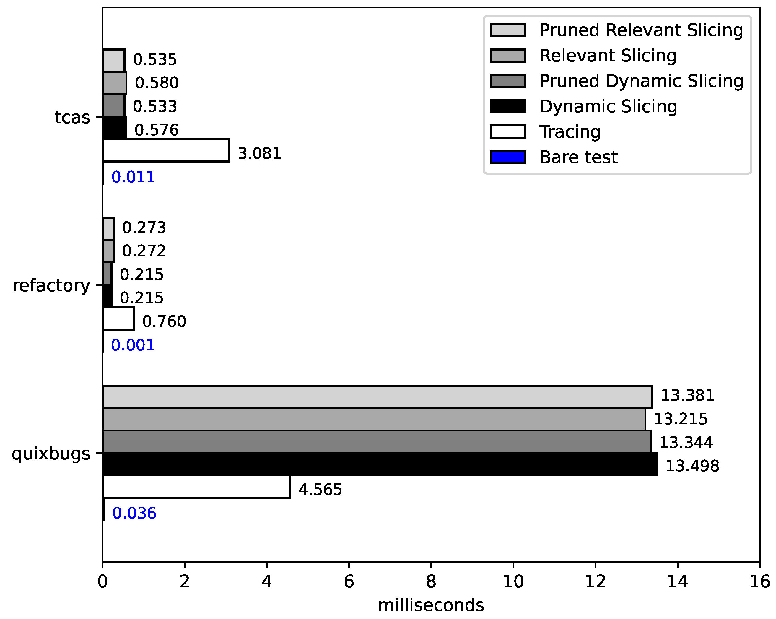
• RQ3: How much additional time is required for tracing and slicing compared to bare execution? What is the computation time overhead of relevant slicing compared to dynamic slicing? What is the computation time overhead of pruned slicing compared to dynamic and relevant slicing? Dynamic slicing requires that the execution of a program be traced. This comes with computation costs. Therefore, we analyze the time required for tracing and slicing and compare it with the bare execution time. Furthermore, we analyze whether relevant slicing and pruned slicing take longer than dynamic slicing.

7.2. Evaluation Metrics

We measure the number of statements in the original programs, execution traces, sets of executed statements, and slices. Before measuring the number of statements, (1) we remove all comments and all standalone string statements, as these do not add any functionality to the program and can be considered as comments, and (2) we convert the programs into an AST and translate them back in order to remove line breaks. This allows us to provide a fair comparison of the evaluated programs.

We use the AST representation to count the number of lines with Boolean expressions and the number of Boolean operators contained in the original programs, set of executed statements, and slices.

We used timeit [39] with 50 repetitions to measure the execution times for executing, tracing, and slicing the different programs.

7.3. Evaluation Environment and Evaluation Restrictions

We evaluated our approach on an AMD^® Ryzen^™ 7 Pro 3700U Processor (2.30 GHz, up to 4.00 GHz Max Boost, 4 Cores, 8 Threads, 4 MB Cache) with 16 GB of RAM, Debian 11 as the operating system, and Python 3.9.

Since our prototype keeps the execution trace in the main memory, we have to restrict the size of the produced execution traces. Given the small size of the input programs, we limit the execution trace length to ${10}^6$ elements and abort the tracing under the assumption that programs reaching this limit are stuck and will not terminate by themselves. Furthermore, we limit the duration for augmenting the source code to five seconds and the duration for tracing, slicing, and code generation to one second each. Evaluation examples that exceed these limits are dismissed.

We decided to use different time limits for the execution of the original and sliced programs of the benchmarks because the programs of the different benchmarks have different structures and, therefore, different execution times. TCAS does not contain recursions (or loops), and therefore we have no time limit for executing the TCAS programs. The programs of the Refactory dataset are small and have reasonable performance; a decision when something hangs indefinitely can be made quickly. Therefore, we set the time limit for executing these programs to 0.1 s. QuixBugs programs heavily rely on recursion and loops and, therefore, often exhibit poor performance. Since we do not want to exclude these slow but executable programs from this benchmark, we set the execution timeout for QuixBugs programs to ten seconds.

7.4. Datasets

Several benchmarks with large and real-world Python 3 programs (e.g., Code4Bench [40], BugSwarm [41], NFBugs [42], SECbench [43], and BugsInPy [44]) are publicly available. However, due to the limitations discussed in Section 6.3, we cannot run our slicer on these benchmarks. Therefore, we decided to use QuixBugs [9], the Refactory dataset [10], and a Python 3 implementation of TCAS (i.e., a program of the Siemens benchmark [11]) to address our research questions.

Table 2. Quantitative description of the benchmarks.

Benchmark	TCAS	Refactory	QuixBugs
Base programs	1	5	31
LOC	91–100	3–115	6–23
Correct program versions	1	1230	31
Faulty program versions	37	2795	31
Test cases	1545	4–17	3–14
Avg. Num. Boolean expressions	14.00	0.20	0.34
Boolean operations	12–15	0–4	0–2

shows the characteristics of the used benchmarks.

QuixBugs originated from the examples of a debugging competition and contains 31 programs. The programs have a simple structure and contain one or two functions, which use recursion or contain (nested) loops. Each program is accompanied by several test cases. All faults can be fixed by changing a single line. In total, we used 62 program versions (31 correct and 31 faulty versions) in our evaluation.

The Refactory dataset [10] is a collection of five programming assignments created by novice students. We removed the duplicate test cases and programs from the benchmark, resulting in 2795 faulty program versions and 1230 correct versions, i.e., 4025 in total. Many of the programs consist of a single function; the programs contain many (nested) loops, but recursion is rarely used.

In our previous work [12], we translated the code of the traffic collision avoidance system (TCAS) from C to Python 3. The program is object-oriented and contains a single class with a constructor and seven methods; one of those methods directly or indirectly calls all other methods. There are no loops but many nested if constructs. While the original C benchmark contains 41 faulty program versions, our Python 3 implementation consists of one correct version and 37 faulty versions because two faulty versions were duplicates and two faulty versions were not reproducible in Python because of Python’s array initialization style. TCAS comes with 1545 test cases.

Pruned slicing reasons over Boolean expressions. In TCAS, on average, 14.00 Boolean expressions are evaluated. In QuixBugs and the Refactory dataset, on average, 0.34 and 0.20 Boolean expressions are evaluated, respectively. Therefore, we expect that the achievable slice reduction through the use of pruned slicing will be highest for the TCAS benchmark.

For each benchmark, we executed each faulty and each correct program version with each test case. We set the timeouts as indicated in Section 7.3. In the next step, we traced the execution steps of the program/test case combinations that terminated.

Table 3. Number of traced program runs and reasons for failures.

Benchmark	TCAS	Refactory	QuixBugs
Successfully executed and traced	58,710	20,836	374
Not executable	-	3144	64
Not supported	-	1161	28
Timeout during tracing	-	-	18

shows the number of successful tracing attempts, as well as the number and reasons for failed tracing attempts. We excluded 3144 program/test case combinations from the Refactory dataset and 64 from QuixBugs because the programs used undefined variables, contained invalid syntax, or did not terminate. Furthermore, we excluded 1161 program/test case combinations from the Refactory dataset and 28 from QuixBugs, which contained language constructs that are not supported by our prototype, and 18 program/test case combinations from QuixBugs, which resulted in a timeout during tracing or exceeded the maximal slice length.

7.5. Results

RQ1: What is the difference between dynamic and relevant slicing with respect to executability, correct results, and slice length? We computed the slices for all program/test case combinations that were successfully traced. We used the return value of the function/method called in the test case as the slicing criterion.

Table 4. Number of successfully sliced program runs and reasons for failures.

Benchmark	TCAS		Refactory		QuixBugs
Slice Type (D = Dynamic, R = Relevant)	D	R	D	R	D	R
Successfully sliced	58,710	58,710	19,683	20,728	367	367
Timeout executing the sliced program	-	-	1044	-	6	6
Other Exception	-	-	76	83	1	1
Sliced result differs from original	-	-	33	25	-	-

shows the number of successful slicing attempts, as well as the number and reasons for failed slicing attempts, separately for dynamic and relevant slicing. For TCAS, all program/test case combinations were successfully sliced. For the Refactory dataset and QuixBugs, the majority of program/test case combinations could be successfully sliced. The dynamic slices of 1044 program/test case combinations from the Refactory dataset resulted in a timeout, but none of the relevant slices resulted in a timeout. This occurred because dynamic slicing sometimes produced incomplete slices, i.e., slices where statements responsible for terminating the loop were missing. There were six program/test case combinations in QuixBugs where both the dynamic and relevant slices resulted in a timeout. There were 76 program/test case combinations where dynamic slicing resulted in other exceptions, and 83 combinations where relevant slicing resulted in other exceptions. There was one program/test case combination in QuixBugs that resulted in an other exception. In the Refactory dataset, there were 33 program/test case combinations where the dynamic slice computed a different result than the original program and 25 where the relevant slices computed different results than the original programs.

Figure 3 shows the average number of statements in the set of executed statements and the dynamic and relevant slices. The data are based on the program/test case combinations where both dynamic and relevant slicing computed the same result as the original program for the variable indicated in the slicing criterion. For TCAS, the number of statements was the same for relevant and dynamic slicing. Both slicing techniques reduced the number of statements compared to the set of executed statements by an average of more than 33% for the TCAS programs.

For the Refactory dataset, dynamic slicing achieved an average reduction of 17.8% compared to the set of executed statements, and relevant slicing achieved a reduction of 8.2%. For QuixBugs, dynamic and relevant slicing achieved reductions of 5.7% and 3.4%, respectively. The programs of the Refactory dataset and QuixBugs are smaller than TCAS. Therefore, their execution traces contained fewer statements. For smaller programs, a smaller reduction with respect to slice size can be achieved.

Figure 4 compares the size of the relevant and dynamic slices point-wise, i.e., for each program/test case combination.

Table 5. Number of program/test case combinations where the relevant slice was greater than, equal to, or smaller than the dynamic slice.

Benchmark	TCAS	Refactory	QuixBugs
Greater	-	6678	45
Equal	58,710	12,955	322
Smaller	-	36	-

provides the number of program/test case combinations where the relevant slice was greater/smaller than or equal to the dynamic slice for all three benchmarks. For TCAS, the relevant and dynamic slices were always identical. For the programs of QuixBugs, the relevant slices were equal to or greater than their dynamic counterparts. For the majority of the program/test case combinations of the Refactory dataset, the relevant slices were equal to or greater than their dynamic counterparts; however, there were 36 program/test case combinations where the relevant slice was slightly smaller than the dynamic slice. We explained this phenomenon in Section 5 (see Example 11).

Summary. The aforementioned results can be summarized as follows:

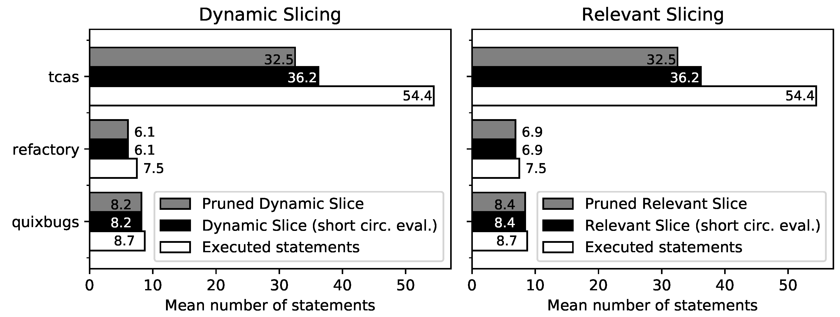
• The dynamic and relevant slices for TCAS are identical. This can be explained by the structure of TCAS: there are no loops, and the then and else branches of the conditionals change the same variable; therefore, relevant slicing has no impact.
• For the Refactory dataset, relevant slicing eliminates the problem of non-terminating slices and reduces the number of slices where the sliced program computes a different result than the original program. However, the average size of the slice increases by 11.2%. For 65.9% of program/test case combinations, the relevant slice is identical to the dynamic slice; for 34.0%, the relevant slice is larger than the dynamic slice; and for 0.2%, it is smaller.
• For QuixBugs, the number of successfully sliced program/test case combinations stays the same, and the average slice size increases by 2.4%. For 87.7% of successfully sliced QuixBugs program/test case combinations, the relevant slice is identical to the dynamic slice, whereas for 12.3%, the size of the slice increases.

RQ2: What reduction with respect to slice length can be achieved by pruning Boolean operations in dynamic and relevant slices? How many Boolean operators are pruned away? How frequently are Boolean operators used in real-world programs? To address these questions, we used all program/test case combinations that could be successfully sliced (see top row of Table 4). Therefore, the figures and tables for dynamic and relevant slicing are based on slightly different datasets within the Refactory dataset.

Figure 5 compares the average sizes of the dynamic/relevant slices to the average sizes of the pruned dynamic/relevant slices. For TCAS, the pruning extension reduced the average size of the dynamic and relevant slices by 10.2%. For the Refactory dataset and QuixBugs, the average sizes of the dynamic and pruned dynamic slices were the same, as were the average sizes of the relevant and pruned relevant slices. The difference in reduction can be explained by the number of Boolean operations in the benchmarks: while TCAS contains many Boolean operations, the programs of the Refactory dataset and QuixBugs contain no or only a few Boolean operations (12–15 for the TCAS versions vs. 0–4 for the Refactory dataset and 0–2 for QuixBugs programs; see Table 2).

Table 6. Number of program/test case combinations where the pruned slices were greater than, equal to, or smaller than the dynamic and relevant slices.

	TCAS	Refactory	QuixBugs
Dynamic Slicing
Greater	-	-	-
Equal	14,107	19,681	367
Smaller	44,603	2	-
Relevant Slicing
Greater	-	-	-
Equal	14,107	20,726	367
Smaller	44,603	2	-

indicates the number of program/test case combinations where the pruned dynamic and relevant slices were greater/smaller than or equal to the dynamic and relevant slices. Figure 6 visually compares the lengths of the dynamic and pruned dynamic slices of each program/test case combination. In 76.0% of TCAS program/test case combinations, pruning achieved a reduction in slice size, and in 24.0%, the size of the slice did not change. For the Refactory dataset, there were only two program/test case combinations where the size of the slice could be reduced using pruned slicing. For QuixBugs, the pruned slices were the same as the original slices. Pruning never increased the slice size in any of the program/test case combinations of the three benchmarks.

Figure 7 illustrates the correlation between the number of Boolean operators in the execution traces and the slice length reduction achieved using pruned slicing. The more Boolean operators executed, the more statements were removed from the slice. Since there were more Boolean operators in the TCAS programs compared to the programs from the Refactory dataset and QuixBugs, pruned slicing worked better for the TCAS programs.

Pruned slicing can help the programmer better understand Boolean expressions by focusing on those parts of the Boolean expression that actually contributed to the outcome of the Boolean expression, as demonstrated in Example 10 in Section 4. Therefore, in Figure 8, we illustrate how many Boolean operators were contained in the dynamic and relevant slices, as well as in their pruned versions. TCAS exhibited the highest reduction, from an average of 4.1 Boolean operators in the dynamic and relevant slices to 1.9 Boolean operators in their pruned versions. For the Refactory dataset, no change was observed. For QuixBugs, the average number of Boolean operators was reduced from 0.3 to 0.2.

Pruned slicing can only reduce the number of statements in a slice when Boolean operators are executed. For this reason, in our previous work [12], we investigated the frequency of Boolean operations in the 20 most downloaded Python packages from PyPI [45] and the 20 most starred Python projects from GitHub [46] (excluding educational and non-English repositories). Figure 9 shows the percentage of lines containing Boolean operations for these 40 projects and our benchmark programs. TCAS exhibits the highest percentage with 10.6%. There is one project, namely python-certifi, that does not contain any Boolean operators. The other projects contain between 0.1% and 3.1% Boolean operators. Since no real-world programs contain anywhere near the percentage of Boolean operators as TCAS, a reduction in the slice size, as achieved for TCAS, would be unlikely for real-world programs. The 40 projects are many times larger than the programs of the Refactory dataset and QuixBugs; therefore, a higher reduction for real-world programs (except python-certifi) compared to QuixBugs and the Refactory dataset might be possible.

Summary. The aforementioned results can be summarized as follows:

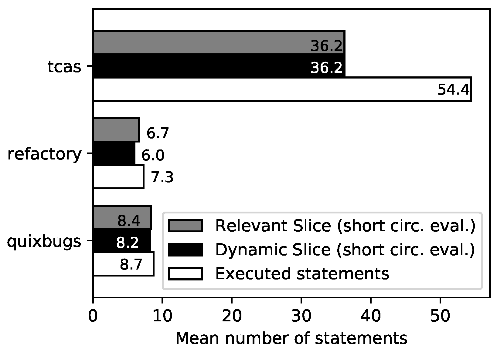
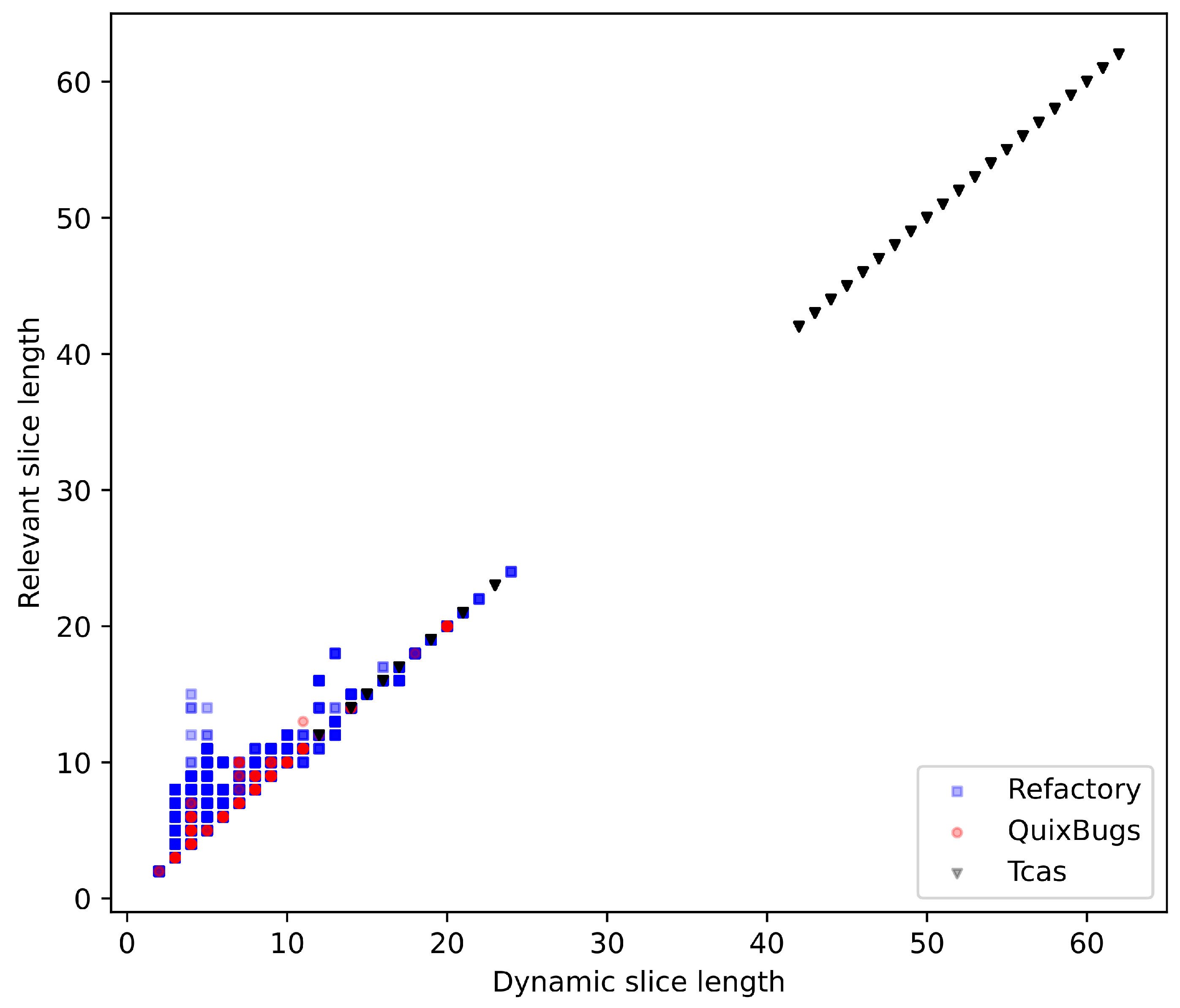
• Pruned slicing reduces the slice size for TCAS by 10.2%. There is no reduction for the Refactory dataset and QuixBugs because only a few Boolean operators are used.
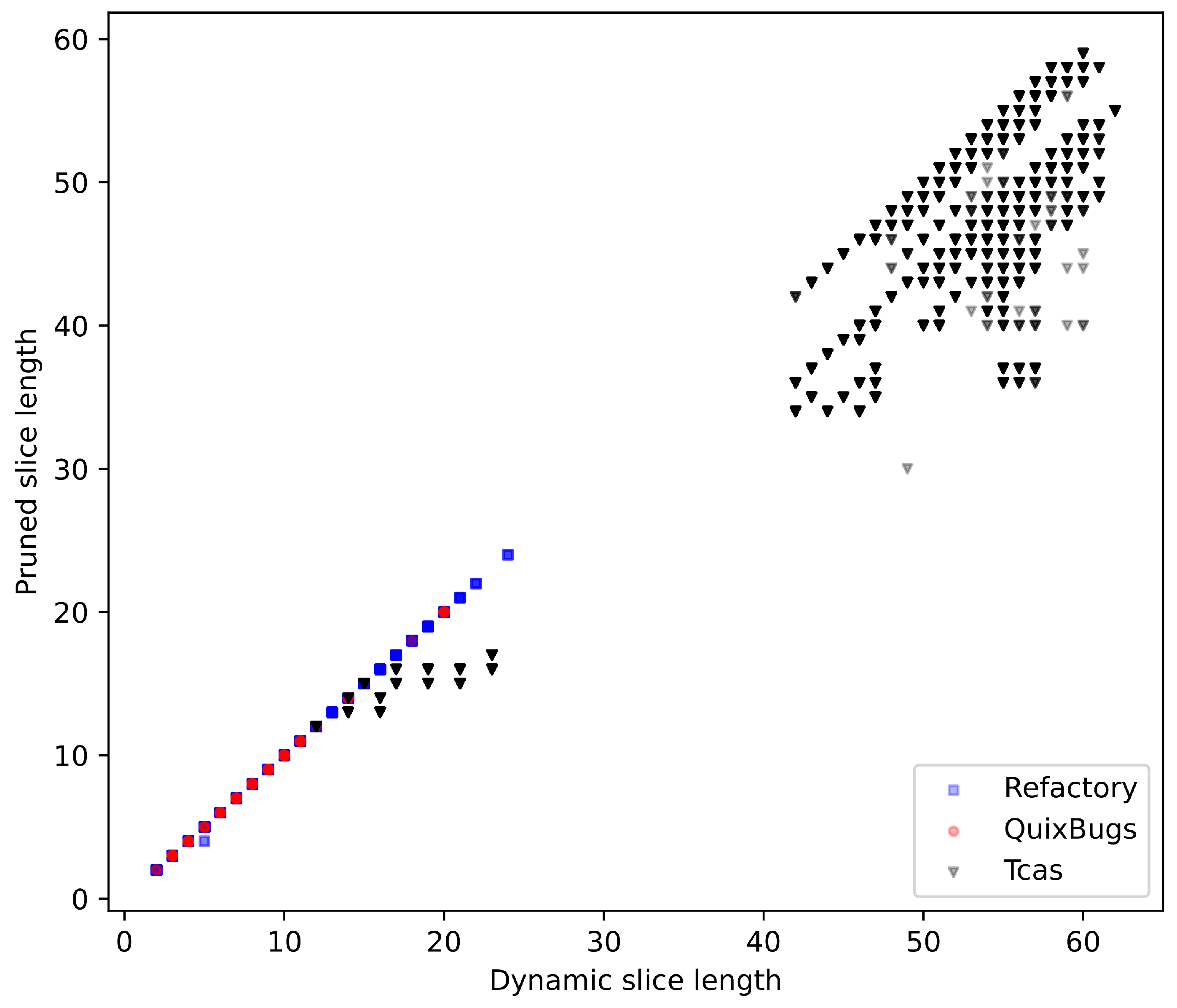
• Pruning can decrease the size of the slice without ever increasing it.
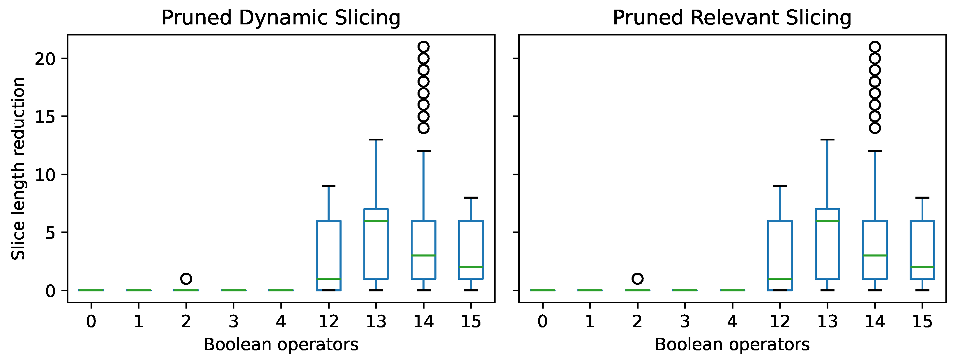
• The more Boolean operators executed, the greater the achievable reduction through the use of pruned slicing.
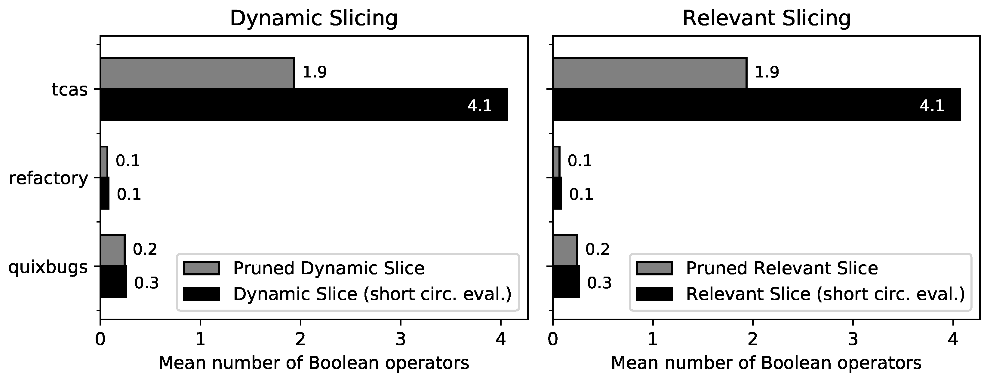
• Pruned slicing can help reduce the number of Boolean sub-terms in the sliced program that need to be investigated by the developer.
• The 40 investigated Python projects show a similar frequency of Boolean operators as the Refactory dataset and QuixBugs but are substantially bigger in terms of LOC.

RQ3: How much additional time is required for tracing and slicing compared to bare execution? What is the computation time overhead of relevant slicing compared to dynamic slicing? What is the computation time overhead of pruned slicing compared to dynamic and relevant slicing? We measured the performance in terms of execution time by averaging 50 repetitions of executing, tracing, and slicing for each program/test case combination. We did not include the execution time for augmenting the source code in the tracing execution time. We used the same traces for dynamic slicing, relevant slicing, and pruned slicing. However, relevant and pruned slicing required more information compared to dynamic slicing: for relevant slicing, we had to analyze the source code to identify the potential relevant variables; for pruned slicing, we had to keep track of the evaluation results of all computed Boolean sub-expressions. We did not investigate the overhead produced for relevant and pruned slicing in the tracing part. The time required for keeping track of the values of the Boolean sub-expressions was included in the tracing execution time. The potential relevant variables were determined during the augmenting process; therefore, the execution time was not measured.

Figure 10 shows the mean execution times for executing, tracing, and computing the dynamic, relevant, and pruned slices. The execution time required for tracing the executed statements was orders of magnitude larger than the bare execution of the programs.

Computing relevant slices took slightly longer than computing dynamic slices for TCAS and the Refactory dataset. This can be explained by the additional checks required for the potential relevant variables (see Section 3.4). Interestingly, computing the relevant slices for QuixBugs required, on average, less time than computing the dynamic slices. We computed the effect size in terms of Cohen’s d for all three benchmarks. The differences were very small for all three benchmarks according to Sawilowsky [47] (TCAS: 0.011; Refactory: 0.086; QuixBugs: 0.005).

Pruned dynamic slicing required slightly less computation time compared to dynamic slicing for TCAS. This can be explained by the size of the set of relevant variables: the set of relevant variables was compared to the set of defined variables for each executed line. With pruned slicing, this set was smaller than with dynamic or relevant slicing, resulting in less time required for comparison. Pruned slicing was as fast as as dynamic slicing for the Refactory dataset. Pruned relevant slicing took longer than relevant slicing for the Refactory dataset and QuixBugs. This can be explained by the fact that pruning hardly ever reduced the set of relevant variables in these benchmarks because of the lack of Boolean expressions, and the additional reasoning came with a small computational overhead. However, the effect sizes in terms of Cohen’s d were again very small (dynamic-pruned dynamic TCAS: 0.135; Refactory: 0.000; QuixBugs: 0.003; and relevant-pruned relevant TCAS: 0.138; Refactory: 0.001; QuixBugs: 0.003).

Figure 11 illustrates that the slice computation time depends on the length of the execution trace. The execution times of the QuixBugs programs clearly highlight this behavior. The QuixBugs programs extensively used recursion and nested loops, and the resulting execution traces were often substantial. Therefore, the higher slice computation time for QuixBugs can be explained by the length of the execution trace. The Pearson coefficient for all three datasets was greater than 0.7, indicating a strong positive correlation (TCAS: 0.955; Refactory: 0.720; QuixBugs: 0.811).

While performance was not our main focus during the implementation of our prototype, the mean tracing and slicing time spans were within an acceptable range, with less than a millisecond for TCAS and the Refactory dataset and a few milliseconds for QuixBugs. We expect that a mature slicer will improve upon these numbers.

Summary. The aforementioned results can be summarized as follows:

• Tracing and slice computation takes orders of magnitude longer than the bare execution.
• The different slicing techniques have similar computation times.
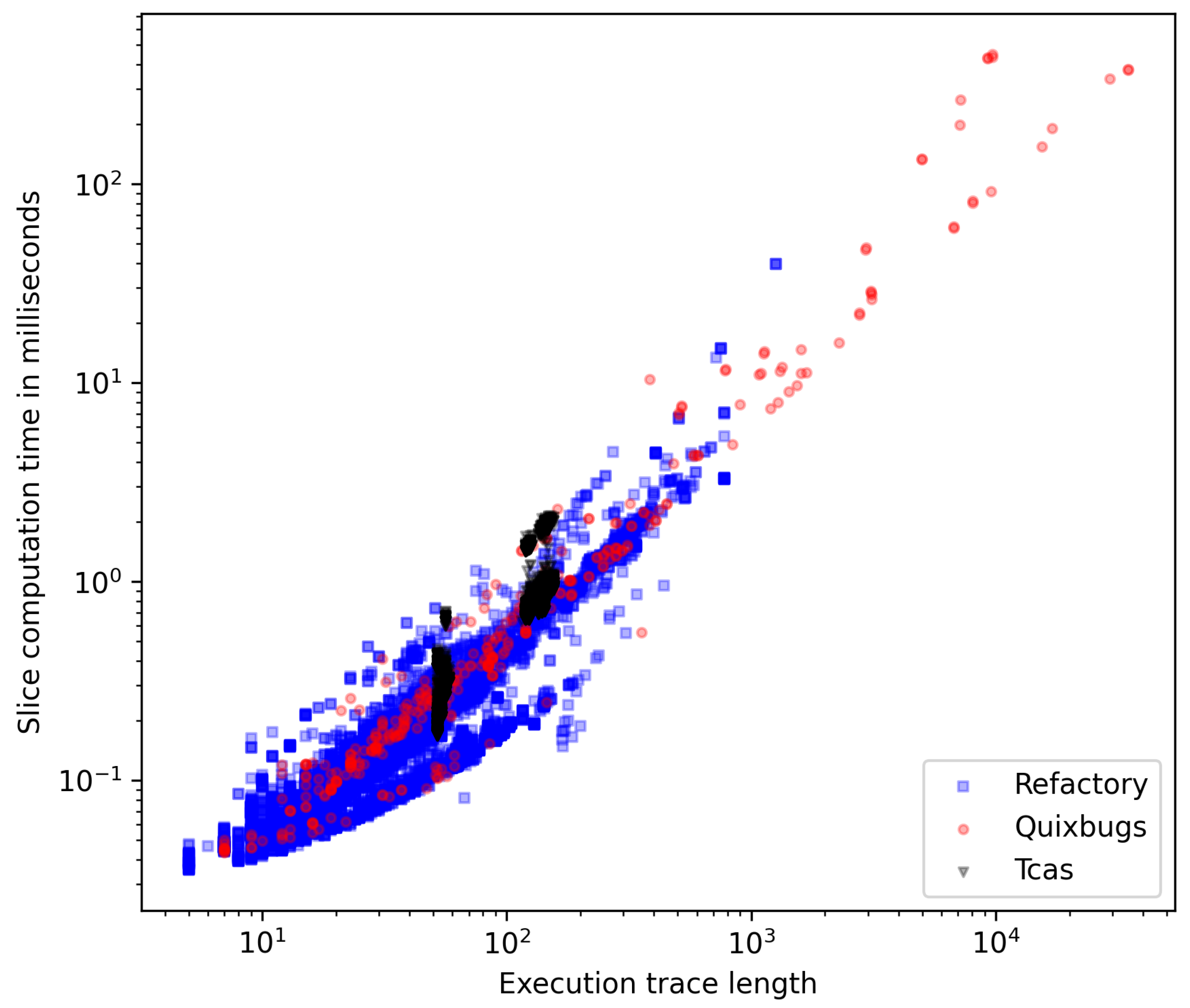
• The time span required for slicing correlates with the length of the execution trace.

7.6. Threats to Validity

The biggest threat to external validity is the representativeness of the used benchmark programs. Since our prototype implementation has many limitations, our evaluation is limited to small programs. We counteracted this threat by using three benchmarks containing programs with different structures such as nested conditionals, loops, and recursive functions. The differences in the structures are reflected in the results. While relevant slicing has no influence on the results of TCAS, it increases the slice size of the Refactory and QuixBugs programs, and while pruned slicing has no or only little effects on the programs of QuixBugs and the Refactory dataset, it reduces the size of the majority of TCAS slices.

To figure out whether the programs represent the structure of real-world programs, we compared the percentage of LOC containing Boolean operators in these three benchmarks to those of 40 open-source Python projects. The comparison revealed that reductions similar to those achieved in the TCAS programs are unrealistic. However, 39 of these 40 projects contain Boolean operators; therefore, pruned slicing might achieve reductions in slice size.

The developed prototype is a major threat to the internal validity of our results. While we designed our prototype with the greatest care, the complexity of the task was immense, particularly when it came to loops, recursive function calls, the immense range of Python language features, and detecting modifications of parameters within function calls. Therefore, bugs cannot be ruled out. To counteract this threat, we used metamorphic testing, which revealed several coding errors and enabled us to fix them. However, it is not possible to detect all coding errors with metamorphic testing.

Metamorphic testing primarily checks whether all statements that should be included in the slice are actually included, but it does not check whether all of the included statements are actually necessary. The latter check is not suitable for our slicer since our algorithm computes small but not necessarily minimal slices. Therefore, it cannot be ruled out that the slices computed by our slicer are larger than actually necessary.

8. Conclusions

In this paper, we have proposed an extension of dynamic and relevant slicing called pruned slicing. Pruned slicing reduces the size of dynamic and relevant slices by reasoning over the evaluation outcome of Boolean sub-expressions and their contribution to the final result of a nested Boolean expression.

We empirically evaluated the average slice sizes of dynamic, relevant, pruned dynamic, and pruned relevant slices for programs taken from three benchmarks containing Python programs, namely TCAS, the Refactory dataset, and QuixBugs. Even though all programs are small, their structures are different, which impacted the results. While the relevant slices of the TCAS programs were equal to the dynamic slices, the average relevant slice sizes of the Refactory and QuixBugs programs increased by 11.2% and 2.4%, respectively. Pruned slicing reduced the slice size of the TCAS programs by an average of 10.2%, but it did not reduce the slice sizes of the Refactory and QuixBugs programs. However, for QuixBugs, the number of Boolean operators was slightly reduced. The differences in execution time for computing dynamic and relevant slices and their pruned counterparts were negligible.

Our evaluation was limited to small programs because of the limitations of our proof-of-concept slicing tool. Developing a dynamic or relevant slicer from scratch that supports all features of a modern programming language is an enormous endeavor. In future work, we will explore the latest dynamic slicers for other programming languages and try to extend promising dynamic slicers with our pruning technique in order to perform our experiments on real-world programs.

Slicing is particularly useful for fault localization, either as a standalone approach or as a preprocessing step for another fault-localization technique. In both scenarios, small slices are preferred over large slices. Even though pruning does not always reduce the size of dynamic and relevant slices, it comes with negligible additional computational costs and should, therefore, be implemented in dynamic and relevant slicers.

References

- Weiser, M. Program Slicing. IEEE Trans. Softw. Eng. 1984, SE-10, 352–357. [Google Scholar] [CrossRef]
- Soha, P.A.; Gergely, T.; Horváth, F.; Vancsics, B.; Beszédes, Á. A Case Against Coverage-Based Program Spectra. In Proceedings of the IEEE Conference on Software Testing, Verification and Validation (ICST), Porto de Galinhas, Brazil, 12–16 April 2023; IEEE: New York, NY, USA, 2023; pp. 13–24. [Google Scholar] [CrossRef]
- Beizer, B. Software Testing Techniques, 2nd ed.; ITP Media: Yas South Abu Dhabi, United Arab Emirates, 1990; p. 580. [Google Scholar]
- Hirsch, T.; Hofer, B. What we can learn from how programmers debug their code. In Proceedings of the 8th International Workshop on Software Engineering Research and Industrial Practice (SER-IP), Madrid, Spain, 4 June 2021; pp. 37–40. [Google Scholar] [CrossRef]
- Korel, B.; Laski, J. Dynamic program slicing. Inf. Process. Lett. 1988, 29, 155–163. [Google Scholar] [CrossRef]
- Agrawal, H.; Horgan, J.; Krauser, E.; London, S. Incremental regression testing. In Proceedings of the Conference on Software Maintenance, Montreal, QC, Canada, 27–30 September 1993; pp. 348–357. [Google Scholar] [CrossRef]
- Pandas. Base.py. Available online: https://github.com/pandas-dev/pandas/blob/a00154dcfe5057cb3fd86653172e74b6893e337d/pandas/core/indexes/base.py (accessed on 11 March 2024).
- Steindl, C. Program Slicing for Programming Languages. Ph.D. Thesis, Johannes Kepler University, Linz, Austria, 1999. [Google Scholar]
- Lin, D.; Chen, A.; Koppel, J.; Solar-Lezama, A. QuixBugs: A Multi-Lingual Program Repair Benchmark Set Based on the Quixey Challenge. In Proceedings of the ACM SIGPLAN International Conference on Systems, Programming, Languages, and Applications: Software for Humanity (SPLASH Companion), Vancouver, BC, Canada, 23–27 October 2017; pp. 55–56. [Google Scholar] [CrossRef]
- Hu, Y.; Ahmed, U.Z.; Mechtaev, S.; Leong, B.; Roychoudhury, A. Re-factoring based program repair applied to programming assignments. In Proceedings of the 34th International Conference on Automated Software Engineering (ASE), San Diego, CA, USA, 11–15 November 2019; pp. 388–398. [Google Scholar] [CrossRef]
- Hutchins, M.; Foster, H.; Goradia, T.; Ostrand, T. Experiments on the effectiveness of dataflow- and control-flow-based test adequacy criteria. In Proceedings of the 16th International Conference on Software Engineering (ICSE), Sorrento, Italy, 16–21 May 1994; pp. 191–200. [Google Scholar] [CrossRef]
- Hirsch, T.; Hofer, B. Pruning Boolean Expressions to Shorten Dynamic Slices. In Proceedings of the 22nd International Working Conference on Source Code Analysis and Manipulation (SCAM), Limassol, Cyprus, 3–4 October 2022; IEEE: New York, NY, USA, 2022; pp. 1–11. [Google Scholar] [CrossRef]
- Bergeretti, J.F.; Carré, B.A. Information-flow and data-flow analysis of while-programs. ACM Trans. Program. Lang. Syst. 1985, 7, 37–61. [Google Scholar] [CrossRef]
- Li, X.; Orso, A. More Accurate Dynamic Slicing for Better Supporting Software Debugging. In Proceedings of the 13th International Conference on Software Testing, Verification and Validation (ICST 2020), Porto, Portugal, 24–28 October 2020; pp. 28–38. [Google Scholar] [CrossRef]
- Agrawal, H.; Demillo, R.A.; Spafford, E.H. Efficient Debugging with Slicing and Backtracking; Technical Report; Purdue University: West Lafayette, IN, USA, 1990. [Google Scholar]
- Tip, F. A Survey of Program Slicing Techniques. J. Program. Lang. 1995, 3, 121–189. [Google Scholar]
- Silva, J. A vocabulary of program slicing-based techniques. ACM Comput. Surv. 2012, 44, 1–41. [Google Scholar] [CrossRef]
- Wong, W.E.; Gao, R.; Li, Y.; Abreu, R.; Wotawa, F. A Survey on Software Fault Localization. IEEE Trans. Softw. Eng. 2016, 42, 707–740. [Google Scholar] [CrossRef]
- Hammacher, C. Design and Implementation of an Efficient Dynamic Slicer for Java. Bachelor’s Thesis, University of Saarland, Saarbrucken, Germany, 2008. [Google Scholar]
- Ahmed, K.; Lis, M.; Rubin, J. Slicer4J: A dynamic slicer for Java. In Proceedings of the 29th ACM Joint Meeting European Software Engineering Conference and Symposium on the Foundations of Software Engineering (ESEC/FSE), Athens, Greece, 23–28 August 2021; pp. 1570–1574. [Google Scholar] [CrossRef]
- Ahmed, K.; Lis, M.; Rubin, J. Mandoline: Dynamic Slicing of Android Applications with Trace-Based Alias Analysis. In Proceedings of the IEEE 14th International Conference on Software Testing, Verification and Validation (ICST 2021), Valencia, Spain, 4–13 April 2021; pp. 105–115. [Google Scholar] [CrossRef]
- Galindo, C.; Perez, S.; Silva, J. A Program Slicer for Java (Tool Paper). In Proceedings of the Software Engineering and Formal Methods, Berlin, Germany, 26–30 September 2022; pp. 146–151. [Google Scholar] [CrossRef]
- Galindo, C.; Pérez, S.; Silva, J. Program slicing of Java programs. J. Log. Algebr. Methods Program. 2023, 130, 100826. [Google Scholar] [CrossRef]
- Nguyen, H.V.; Kästner, C.; Nguyen, T.N. Cross-language program slicing for dynamic web applications. In Proceedings of the 10th Joint Meeting of the European Software Engineering Conference and the ACM SIGSOFT Symposium on the Foundations of Software Engineering (ESEC/FSE), Lisbon, Portugal, 5–9 September 2015; pp. 369–380. [Google Scholar] [CrossRef]
- Stiévenart, Q.; Binkley, D.W.; Roover, C.D. Static stack-preserving intra-procedural slicing of webassembly binaries. In Proceedings of the 44th International Conference on Software Engineering (ICSE ’22), Pittsburgh, PA, USA, 22–27 May 2022; pp. 2031–2042. [Google Scholar] [CrossRef]
- Galindo, C.; Pérez, S.; Silva, J. Exception-sensitive program slicing. J. Log. Algebr. Methods Program. 2023, 130, 100832. [Google Scholar] [CrossRef]
- Galindo, C.; Pérez, S.; Silva, J. Program Slicing Techniques with Support for Unconditional Jumps. In Proceedings of the 23rd International Conference on Formal Engineering Methods (ICFEM 2022), Madrid, Spain, 24–27 October 2022; pp. 123–139. [Google Scholar] [CrossRef]
- Nanda, M.G.; Ramesh, S. Interprocedural slicing of multithreaded programs with applications to Java. ACM Trans. Program. Lang. Syst. 2006, 28, 1088–1144. [Google Scholar] [CrossRef]
- Galindo, C.; Llorens, M.; Pérez, S.; Silva, J. Slicing Shared-Memory Concurrent Programs The Threaded System Dependence Graph Revisited. In Proceedings of the IEEE International Conference on Software Maintenance and Evolution (ICSME), Bogota, Colombia, 1–6 October 2023; pp. 73–83. [Google Scholar] [CrossRef]
- Ghosh, D.; Singh, J. A dynamic slicing-based approach for effective SBFL technique. Int. J. Comput. Sci. Eng. 2021, 24, 98–107. [Google Scholar] [CrossRef]
- Soremekun, E.; Kirschner, L.; Böhme, M.; Zeller, A. Locating Faults with Program Slicing: An Empirical Analysis. arXiv 2021, arXiv:2101.03008. [Google Scholar] [CrossRef]
- Messaoudi, S.; Shin, D.; Panichella, A.; Bianculli, D.; Briand, L.C. Log-Based Slicing for System-Level Test Cases. In Proceedings of the International Symposium on Software Testing and Analysis (ISSTA), Aarhus, Denmark, 12–16 July 2021; pp. 517–528. [Google Scholar]
- de Vos, M.; Pouwelse, J. ASTANA: Practical String Deobfuscation for Android Applications Using Program Slicing. arXiv 2021, arXiv:2104.02612. [Google Scholar]
- Wang, S.; Wang, X.; Sun, K.; Jajodia, S.; Wang, H.; Li, Q. GraphSPD: Graph-Based Security Patch Detection with Enriched Code Semantics. In Proceedings of the IEEE Symposium on Security and Privacy (SP), San Francisco, CA, USA, 21–25 May 2023; pp. 2409–2426. [Google Scholar] [CrossRef]
- Zhang, Z.; Lei, Y.; Yan, M.; Mao, X.; Su, T.; Yu, Y. Influential Global and Local Contexts Guided Trace Representation for Fault Localization. ACM Trans. Softw. Eng. Methodol. 2022, 1, 27. [Google Scholar] [CrossRef]
- Home Assistant: Network.py. Available online: https://github.com/home-assistant/core/blob/1242456ff1fc8f70ff48503f91d6d54d9a46cfbc/homeassistant/helpers/network.py (accessed on 11 March 2024).
- Python Documentation: Abstract Syntax Tree. Available online: https://docs.python.org/3/library/ast.html (accessed on 11 March 2024).
- Segura, S.; Fraser, G.; Sanchez, A.B.; Ruiz-Cortes, A. A Survey on Metamorphic Testing. IEEE Trans. Softw. Eng. 2016, 42, 805–824. [Google Scholar] [CrossRef]
- Python Documentation: Timeit—Measure Execution Time of Small Code Snippets. Available online: https://docs.python.org/3/library/timeit.html (accessed on 11 March 2024).
- Majd, A.; Vahidi-Asl, M.; Khalilian, A.; Baraani-Dastjerdi, A.; Zamani, B. Code4Bench: A multidimensional benchmark of Codeforces data for different program analysis techniques. J. Comput. Lang. 2019, 53, 38–52. [Google Scholar] [CrossRef]
- Tomassi, D.A.; Dmeiri, N.; Wang, Y.; Bhowmick, A.; Liu, Y.C.; Devanbu, P.T.; Vasilescu, B.; Rubio-Gonzalez, C. BugSwarm: Mining and Continuously Growing a Dataset of Reproducible Failures and Fixes. In Proceedings of the International Conference on Software Engineering (ICSE), Montreal, QC, Canada, 25–31 May 2019; pp. 339–349. [Google Scholar] [CrossRef]
- Radu, A.; Nadi, S. A dataset of non-functional bugs. In Proceedings of the International Working Conference on Mining Software Repositories (MSR), Montreal, QC, Canada, 26–27 May 2019; pp. 399–403. [Google Scholar] [CrossRef]
- Reis, S.; Abreu, R. SECBENCH: A Database of Real Security Vulnerabilities. In Proceedings of the International Workshop on Secure Software Engineering in DevOps and Agile Development (SecSE), Oslo, Norway, 11–15 September 2017; pp. 70–85. [Google Scholar]
- Widyasari, R.; Sim, S.Q.; Lok, C.; Qi, H.; Phan, J.; Tay, Q.; Tan, C.; Wee, F.; Tan, J.E.; Yieh, Y.; et al. BugsInPy: A database of existing bugs in Python programs to enable controlled testing and debugging studies. In Proceedings of the 28th ACM Joint Meeting on European Software Engineering Conference and Symposium on the Foundations of Software Engineering (ESEC/FSE), New York, NY, USA, 8–13 November 2020; pp. 1556–1560. [Google Scholar] [CrossRef]
- PyPiStats: Most Downloaded PyPI Packages. Available online: https://pypistats.org/top (accessed on 1 June 2021).
- GitHub Topics: Python. Available online: https://github.com/topics/python?l=python&o=desc&s=stars (accessed on 1 June 2021).
- Sawilowsky, S.S. New Effect Size Rules of Thumb. J. Mod. Appl. Stat. Methods 2009, 8, 597–599. [Google Scholar] [CrossRef]