Modeling and Analyzing Reaction Systems in Maude

Abstract

Reaction Systems (RSs) are a successful computational framework for modeling systems inspired by biochemistry. An RS defines a set of rules (reactions) over a finite set of entities (e.g., molecules, proteins, genes, etc.). A computation in this system is performed by rewriting a finite set of entities (a computation state) using all the enabled reactions in the RS, thereby producing a new set of entities (a new computation state). The number of entities in the reactions and in the computation states can be large, making the analysis of RS behavior difficult without a proper automated support. In this paper, we use the Maude language—a programming language based on rewriting logic—to define a formal executable semantics for RSs, which can be used to precisely simulate the system behavior as well as to perform reachability analysis over the system computation space. Then, by enriching the proposed semantics, we formalize a forward slicer algorithm for RSs that allows us to observe the evolution of the system on both the initial input and a fragment of it (the slicing criterion), thus facilitating the detection of forward causality and influence relations due to the absence/presence of some entities in the slicing criterion. The pursued approach is illustrated by a biological reaction system that models a gene regulation network for controlling the process of differentiation of T helper lymphocytes.

1. Introduction

Reaction systems (RSs) [1,2] are a computational framework inspired by the functioning of living cells and by biochemistry. Their constituents are a finite set of entities (a background set) and a finite set of reactions. Each reaction is a triple that consists of a set of entities whose presence is needed to enable the reaction, called reactants; a set of entities whose absence is needed to enable the reaction, called inhibitors; and a set of entities that are produced when the reaction takes place, called products. All entities must be included in a fixed background set. Applications of RSs are very general and range from the modeling of biological phenomena [3,4,5] to molecular chemistry [6]. The classical behavior of RSs is defined as a rewriting system whose states are sets of entities (those produced at the previous step, possibly joined with others provided by an external context that models the interaction with the environment).

1.1. Problem Statement

The number of entities in the reactions and in the computation states can be large and difficult to verify for its correctness by the users. Thus, automated verification and debugging tools can be very helpful.

The design of RSs for modeling some natural phenomenon is often conducted by domain experts to validate their hypotheses and requires some degree of abstraction. False assumptions or inaccuracies may be introduced as early as the design stage. Moreover, writing reactions is an error-prone activity, and verifying their behavior can be difficult even for RSs with just a few dozens of entities and reactions. For example, if some mistake is made at the design level and some inexplicable result is observed during the simulation, then an analysis of the computation may be necessary to understand the nature of the problem.

1.2. The Approach

Program slicing is a traditional method used to circumscribe the key parts of a program that may be responsible for a specific unexpected outcome. Originally, slicing was defined as a static technique by [7]. Later, Ref. [8] expanded upon this concept by introducing dynamic program slicing, which aids in the debugging process by identifying—at runtime—those fragments of a program containing the flawed code. Dynamic program slicing has been applied to several programming paradigms (see Silva [9] for a survey).

The idea explored in this paper is to define and implement a novel dynamic slicing technique, which builds on top of a formal executable semantics for RSs, suitable for analyzing RS processes. Both the RS semantics and the slicing algorithm will be specified in Maude [10]: a high-level programming language and system based on the rewriting logic framework of [11]. Maude [12] supports functional, concurrent, logic, and object-oriented computations and provides equational rewriting and reasoning modulo user-defined equations and algebraic axioms such as associativity, commutativity, and identity. Maude is well-suited to specify software systems. In fact, a Maude specification combines a set of rewrite rules R, which specifies the state transitions of a system, with an equational theory $\mathcal{E}$ that specifies system states as terms of an algebraic data type. The equations in $\mathcal{E}$ are implicitly oriented from left to right as rewrite rules and operationally used as simplification rules to perform rewriting modulo equations and axioms.

1.3. Contribution

The main contributions of this paper are listed below.

• We provide an elegant and concise Maude specification that rigorously formalizes an executable semantics for reaction systems. We also prove correctness of our implementation with regard to the usual set-theoretic reaction system characterization.
• We apply the previous formalization to a biological model for gene regulation and we take advantage of the rich Maude development environment [12] to support and simplify the analysis phase. More specifically, we first illustrate how the Maude built-in search facility can be used to perform reachability analysis on the model. Then, we employ the ANIMA system [13]—a visual program explorer for Maude computations that we developed in a previous work—to provide an incremental view of the evolution of a reaction system. In ANIMA, system biologists can explore the computation space of RSs in a stepwise manner by expanding state transitions one at a time, thereby focusing on selected aspects of the biological processes.
• By enriching the reaction system semantics, we also define a forward slicing algorithm for RSs and we formally prove its correctness. Forward slicing is a powerful tool to detect (forward) causality and influence relations among the entities produced in a biological model. It shows how (parts of) an initial input affect the production of (parts of) the output and helps estimate which input data need to be modified to accomplish a change in the outcome. Similarly to [2,14], our approach considers context-independent RSs (that is, RSs where the environment only provides a set of initial entities $C_0$). More precisely, our forward slicing methodology requires the user to select a subset $C_0^{\prime }$ of the initial input $C_0$ specifying the entities to be observed. Then, it proceeds by producing a computation that encodes two reaction system processes that progress in parallel: the original process that stems from $C_0$ and a secondary process (the sliced one) that originates from $C_0^{\prime }$ and that includes only the entities and reactions which are related to the partial input $C_0^{\prime }$. This way, the two processes can be easily compared to detect errors and/or causality relations.
• By applying our forward slicing technique to a gene regulation model, we show how computation states can be drastically reduced in size, favoring the system comprehension and detection of influence relations among entities.

1.4. Organization

In Section 2, we recall the basics of RSs. In Section 3, we introduce some preliminary notions on rewriting logic and Maude. We assume some basic knowledge of term rewriting [15] and some familiarity with the Maude language. In Section 4, we define a Maude specification that provides a precise execution model for RSs and we formally prove its correspondence with regard to the set-theoretic representation of reaction systems presented in Section 2. In Section 5, the Maude specification in Section 4 is used to explore and analyze an RS that specifies a gene regulation network. In Section 6, we first define a forward slicing algorithm for RSs and prove its correctness. Then, we show how our forward slicing method works in practice using the gene regulation example in Section 5. We discuss some related work in Section 7 and future work in Section 8, together with concluding remarks.

2. Reaction Systems

Let us recall some basic notions about reaction systems that are relevant to this work. For a full discussion on this topic, it is possible to consult [1,2].

An entity is a generic element (e.g., molecules, ions, atoms, and other chemicals) that may be present in biochemical reactions. Let S be a finite set of entities (the background set). A reaction in S is a triple $(R,I,P)$, where R, I, and P are finite sets of entities such that $R,I,P\subseteq S$ and $R\cap I=\varnothing$. The sets R, I, P, respectively, model sets of reactants, inhibitors, and products of the reaction. By $rac\left(S\right)$, we denote the set of all reactions on S.

Informally, a reaction can take place whenever all of its reactants are present in a given state while none of its inhibitors are present. If this happens, the reaction is enabled and creates its products. More formally, given a set $T\subseteq S$, a reaction $a=(R_a,I_a,P_a)$ is enabled by T, denoted $e{n}_a\left(T\right)$, if and only if $T\subseteq R_a$ and $T\cap I_a=\varnothing$. The result (or outcome) of a on T is defined by

$$re{s}_a\left(T\right)=\left\{\begin{array}{cc}{P}_a\hfill & \mathrm{if} e{n}_a\left(T\right)\hfill \\ \varnothing \hfill & otherwise\hfill \end{array}\right.$$

We assume that for each reaction $(R,I,P)$, R, I, and P are non-empty. This guarantees that, for each reaction a, there is always at least one product of a that is produced by at least one reactant of a. Note that, if an entity in a state is not sustained by at least one reaction which produces it, then it will disappear in the following state. This behavior reflects one of the core assumption of RSs, namely, the no permanency principle [2]. In other words, an entity from a current state vanishes unless it is produced by the system.

Given a set of reactions $A\subseteq rac\left(S\right)$ and a set of entities $T\subseteq S$, the result (or outcome) of A on T is ${\bigcup }_{a\in A}re{s}_a\left(T\right)$. This definition assumes that there is no conflict on the available resources. Indeed, RSs enjoy the threshold supply principle [2]: either an entity is present in the state and there is “enough” of it, or an entity is not present. To put it differently, two or more reactions that are enabled by T always generate their products, even if they share some entities, because there is always a sufficient amount of reactants in T to activate all the enabled reactions. Note that this assumption implies a major difference with standard models of concurrent systems, such as Petri nets.

Definition 1.

A reaction system (RS, in short) is a pair $\mathcal{A}=(S,A)$ such that S is a finite set of entities and $A\subseteq rac\left(S\right)$.

The dynamics of reaction systems is defined through the notion of interactive process, that is, a process that may react to external stimuli. More formally,

Definition 2.

Let $\mathcal{A}=(S,A)$ be a reaction system and let $n\ge 0$ be an integer, an n-step interactive process in $\mathcal{A}$ is a pair $\pi =(\gamma ,\delta )$ such that $\gamma =C_0,C_1,\dots ,C_n$ and $\delta =D_0,D_1,\dots ,D_n$ where

1.

$C_i,D_i\subseteq S$, for $i=0,\dots ,n$;

2.

$D_0=\varnothing$;

3.

$D_i=re{s}_A(D_{i-1}\cup C_{i-1})$, for $i=1,\dots ,n$.

The sequence $\gamma$ is called context sequence and represents the environment that may interact with the RS, while $\delta$ is the result sequence which is completely determined by reactions in A and contexts in $\gamma$.

It is worth noting that Definition 2 models reaction systems as open systems that may react to external inputs which are provided by the context sequence. Therefore, distinct context sequences may lead to distinct outcomes for the same RS $\mathcal{A}$, as illustrated in the following example.

Example 1.

Let $\mathcal{A}=(S,A)$ be a RS such that $S=\{\mathsf{a},\mathsf{b},\mathsf{c}\}$ and $A=\{a_1,a_2\}$ where

$$\begin{array}{cc}\hfill a_1& =\left(\right\{\mathsf{a},\mathsf{b}\},\{\mathsf{c}\},\{\mathsf{a}\left\}\right),\hfill \\ \hfill a_2& =\left(\right\{\mathsf{a}\},\{\mathsf{b}\},\{\mathsf{c}\left\}\right).\hfill \end{array}$$

Consider a three-step interactive process $\pi =(\gamma ,\delta )$ where $\gamma =C_0,C_1,C_2$ with $C_0=\{\mathsf{a},\mathsf{b}\}$, $C_1=\left\{\mathsf{c}\right\}$ and $C_2=\left\{\mathsf{b}\right\}$. Then, $\delta =D_0,D_1,D_2=\varnothing$, $\left\{\mathsf{a}\right\}$, $\left\{\mathsf{c}\right\}$.

Now, consider the three-step interactive process ${\pi }^{\prime }=({\gamma }^{\prime },{\delta }^{\prime })$, where the context sequence ${\gamma }^{\prime }=C_0^{\prime },$$C_1^{\prime },C_2^{\prime }=\{\mathsf{a},\mathsf{b}\},\{\mathsf{b},\mathsf{c}\},\left\{\mathsf{b}\right\}$ is a slight mutation of γ. Then, we obtain ${\delta }^{\prime }=D_0^{\prime },D_1^{\prime },D_2^{\prime }=\varnothing ,$$\left\{\mathsf{a}\right\},\varnothing$.

Given an interactive process $\pi =(\gamma ,\delta )$ such that $\gamma =C_0,C_1,\dots ,C_n$ and $\delta =D_0,$$D_1,\dots ,D_n$, we say that $\pi$ is a context-independent process if $C_i\subseteq D_i$, for $i=1,\dots ,n$. In this special case, the result sequence $\delta$ is completely determined by the initial context $C_0$. More specifically, $D_1$ only depends on $C_0$, and $D_{i+1}$ only depends on $D_i$, with $i=1,\dots ,(n-1)$. For this reason, we often denote a context-independent process as $\pi =(C_0,\delta )$.

3. Software Systems in Maude

The Maude system [10,12] is a formal language and tool set based on rewriting logic. Rewriting logic  [11] is a logical formalism that is based on two simple ideas: states of a system are represented as terms of an algebraic data type, specified in a Maude equational theory, and the behavior of a system is given by local transitions between states described by rewrite rules.

An equational theory specifies data types by declaring operators whose composition builds complex data structures from simpler ones. Maude equational theories are order-sorted: this means that operators have a typed structure over a set of sorts $\mathsf{\Gamma }$, and there exists a (possibly empty) poset (Γ, <) that models subsort relations between the sorts in $\mathsf{\Gamma }$. An operator f in an equational theory is specified in prefix notation by using the syntax $\mathtt{op}\mathtt{f}:{\mathtt{s}}_{\mathtt{1}}\dots {\mathtt{s}}_{\mathtt{n}}\to \mathtt{s}$, $\mathtt{n}\ge \mathtt{0}$, where ${\mathtt{s}}_{\mathtt{1}}\dots {\mathtt{s}}_{\mathtt{n}}$ denotes the sequence of argument sorts (i.e., the arity of $\mathtt{f}$), and $\mathtt{s}$ is the sort of the return value (the keyword $\mathtt{ops}$ can be used to declare multiple operators with the same type structure: e.g., $\mathtt{ops}\mathtt{f}\mathtt{g}\mathtt{h}:{\mathtt{s}}_{\mathtt{1}}\to {\mathtt{s}}_{\mathtt{2}}$). When the arity of $\mathtt{f}$ is the empty sequence, $\mathtt{f}$ is called constant. An operator can be specified in mixfix notation by using underscores as place holders for the input arguments (e.g., $\_\otimes \_:{\mathtt{s}}_{\mathtt{1}}{\mathtt{s}}_{\mathtt{2}}\to \mathtt{s}$). Binary operators may have attached an axiom declaration that specifies any combinations of algebraic laws such as associativity (assoc), commutativity (comm), and identity (id). By $\mathtt{Ax}$, we denote the set of all axioms attached to the operators in the equational theory. Variables are introduced together with their sort by means of the keyword $\mathtt{var}$ for a single variable declaration or the keyword $\mathtt{vars}$ for multiple declarations on a single line.

Equations in an equational theory define functions that can be used in term simplification. A term is a variable or an application of an operator to a list of terms. Assuming the equations fully define all the specified functions, each term $\mathtt{t}$ has a canonical form (modulo $\mathtt{Ax}$), which is denoted by ${\mathtt{t}}_{{\downarrow }_{\mathcal{E}}}$. The canonical form ${\mathtt{t}}_{{\downarrow }_{\mathcal{E}}}$ is obtained by using the equations, oriented left to right, to rewrite $\mathtt{t}$ (modulo $\mathtt{Ax}$) until no more rewrites are possible. Equations are specified by using the following syntax: $\mathtt{eq}\mathtt{l}=\mathtt{r}$, where $\mathtt{l}$ and $\mathtt{r}$ are terms whose sorts belong to the same connected component of $(\mathsf{\Gamma },<)$. An equational theory $\mathcal{E}$ in Maude is specified by a functional module, which is delimited by keywords $\mathtt{fmod}$ and $\mathtt{endfm}$, that contains sort, variable, operator and equation definitions.

Example 2.

The functional module of Listing 1 specifies an equational theory that models sets of entities. Line 4 defines three atomic entities via the constants $\mathtt{a}$, $\mathtt{b}$, $\mathtt{c}$ of sort $\mathtt{Entity}$. Sets are terms of sort $\mathtt{Entities}$ whose form is ${\mathtt{e}}_{\mathtt{1}}\dots {\mathtt{e}}_{\mathtt{n}}$, where each ${\mathtt{e}}_{\mathtt{i}}$ is a term of sort $\mathtt{Entity}.$ Sets are built using the associative and commutative operator $\_\_$ with identity $\mathtt{empty}$, plus the equation in Line 10 that models idempotence to allow for multiple occurrences of the same entity to be automatically simplified. The identity $\mathtt{empty}$ specifies the empty set. Note that, thanks to the subsort relation of Line 3, each term of sort $\mathtt{Entity}$ is also a term of sort $\mathtt{Entities}$; hence, atomic entities can be also interpreted as singletons.

Finally, Lines 11–12 provide an equational definition for the Boolean function $\mathtt{isEmpty}\left(\mathtt{E}\right)$ that verifies whether the set $\mathtt{E}$ is empty. Note that the attribute $\mathtt{owise}$ in Line 12 applies the equation in Line 12 whenever equation in Line 11 cannot be applied (that is, when $\mathtt{E}$ is not empty).

Canonical forms of a term $\mathtt{t}$ in Maude can be computed via the $\mathtt{red}$ command, that simplifies $\mathtt{t}$ using the equations and axioms in the functional module. For instance,

Maude> red a b a a c .

reduce in ENTITYSET : a b a a c .

rewrites: 2 in 0ms cpu (0ms real) (2000000 rewrites/second)

result Entities: a b c

and

Maude> red isEmpty(a b a a c) .

reduce in ENTITYSET : isEmpty(a b a a c) .

rewrites: 3 in 0ms cpu (0ms real) (3000000 rewrites/second)

result Bool: false

Listing 1. An equational theory for modeling sets of entities.

1 fmod ENTITYSET is

2   sorts Entity Entities .

3   subsort Entity < Entities .

4   ops a b c : -> Entity .

5   op empty : -> Entities .

6   op __ : Entities Entities -> Entities [assoc comm id: empty] .

7   op isEmpty : Entities -> Bool .

8   var x : Entity .

9   var E : Entities .

10   eq x x = x .

11   eq isEmpty(empty) = true .

12   eq isEmpty(E) = false [owise] .

13 endfm

A conditional rewrite rule is an expression of the form $\mathtt{crl}\left[\mathtt{lbl}\right]\mathtt{l}=>\mathtt{r}\mathtt{if}\mathtt{C}$, where $\mathtt{lbl}$ is a label that identifies the rule, $\mathtt{l}$ and $\mathtt{r}$ are terms whose sorts belong to the same connected component of $(\mathsf{\Gamma },<)$, and $\mathtt{C}$ is a (possibly empty) conjunction of Boolean expressions. When the condition $\mathtt{C}$ is empty, we simply write $\mathtt{rl}\left[\mathtt{lbl}\right]:\mathtt{l}=>\mathtt{r}$.

A rewrite theory $\mathcal{R}$ consists of an equational theory $\mathcal{E}$ plus a set of rewrite rules R. Rewrite theories in Maude are specified by system modules (delimited by keywords $\mathtt{mod}$ and $\mathtt{endm}$), which include a sequence of rewrite rules and one or more functional modules encoding a given equational theory. A rewrite theory is also called Maude specification.

Concurrent as well as nondeterministic software systems can be formalized through rewrite theories.

A software system, modeled as a rewrite theory, evolves by rewriting terms using equational rewriting, i.e., rewriting with the rewrite rules in R modulo the equations and axioms in $\mathcal{E}$ [11]. More precisely, (system) computations correspond to (possibly infinite) rewrite sequences ${\mathtt{t}}_{\mathtt{0}}{\stackrel{{\mathtt{r}}_{\mathtt{0}}}{⟶}}_{\mathit{R},\mathcal{E}}{\mathtt{t}}_{\mathtt{1}}{\stackrel{{\mathtt{r}}_{\mathtt{1}}}{⟶}}_{\mathit{R},\mathcal{E}}\dots$, where $\mathtt{t}{\stackrel{\mathtt{r}}{⟶}}_{\mathit{R},\mathcal{E}}{\mathtt{t}}^{\prime }$ denotes a transition (modulo $\mathcal{E}$) from term $\mathtt{t}$ to ${\mathtt{t}}^{\prime }$ via the rewrite rule of R that is uniquely labeled with $\mathtt{r}$. The length of a finite computation $\mathcal{C}$ is the number of transitions it includes. Hence, the length of the computation ${\mathtt{t}}_{\mathtt{0}}{\stackrel{{\mathtt{r}}_{\mathtt{0}}}{⟶}}_{\mathit{R},\mathcal{E}}{\mathtt{t}}_{\mathtt{1}}\dots {\stackrel{{\mathtt{r}}_{\mathtt{n}-\mathtt{1}}}{⟶}}_{\mathit{R},\mathcal{E}}{\mathtt{t}}_{\mathtt{n}}$ is n.

Note that each single transition $\mathtt{t}{\stackrel{\mathtt{r}}{⟶}}_{\mathit{R},\mathcal{E}}{\mathtt{t}}^{\prime }$ is actually implemented as a rewrite chain $\mathtt{t}{\to }_{\mathcal{E}}^{\ast }\left({\mathtt{t}}_{{\downarrow }_{\mathcal{E}}}\right)\stackrel{\mathtt{r}}{⟶}{\mathtt{t}}^{\prime }$, where the prefix $\mathtt{t}{\to }_{\mathcal{E}}^{\ast }{\mathtt{t}}_{{\downarrow }_{\mathcal{E}}}$ is an equational simplification sequence that rewrites $\mathtt{t}$ into its canonical form ${\mathtt{t}}_{{\downarrow }_{\mathcal{E}}}$ using $\mathcal{E}$; then, ${\mathtt{t}}_{{\downarrow }_{\mathcal{E}}}$ is rewritten to ${\mathtt{t}}^{\prime }$ using a rewrite rule $\mathtt{r}$ in R. Although advisedly omitted in our notation, all rewrites in the chain (either applying $\mathtt{r}$ or any of the equations in $\mathcal{E}$) are performed modulo the equational axioms of $\mathcal{E}$. Terms in a computations are also called states.

Example 3.

Consider the toy rewrite theory ${\mathcal{R}}_{toy}$ that is encoded in the Maude system module of Listing 2. ${\mathcal{R}}_{toy}$ includes the equational theory ${\mathcal{E}}_{toy}$ of Listing 1 via the import command $\mathtt{pr}$ at Line 2. ${\mathcal{E}}_{toy}$ is used to model states as sets of entities. The rewrite theory also contains three rewrite rules that allow for the current set (state) to be modified by removing an entity ($\mathtt{a}$, $\mathtt{b}$ or $\mathtt{c}$) from it. For instance, the following one-step computation can be produced in ${\mathcal{R}}_{toy}$:

$$\mathtt{b}\mathtt{b}\mathtt{a}\mathtt{c}\mathtt{a}{\stackrel{\mathtt{del}-\mathtt{a}}{⟶}}_{{\mathit{R}}_{\mathit{toy}},{\mathcal{E}}_{\mathtt{toy}}}\mathtt{b}\mathtt{c}$$

which is implemented by first simplifying the initial state $\mathtt{b}\mathtt{b}\mathtt{a}\mathtt{c}\mathtt{a}$ into the canonical form $\mathtt{a}\mathtt{b}\mathtt{c}$ by using the equation $\mathtt{eq}\mathtt{x}\mathtt{x}=\mathtt{x}$, associativity and commutativity of the binary operator $\_\_$. Then, the rewrite rule del-a is applied to the canonical form $\mathtt{a}\mathtt{b}\mathtt{c}$ to obtain $\mathtt{b}\mathtt{c}$. In symbols, $\mathtt{b}\mathtt{b}\mathtt{a}\mathtt{c}\mathtt{a}{\to }_{\mathcal{E}}^{\ast }\mathtt{a}\mathtt{b}\mathtt{c}\stackrel{\mathtt{del}-\mathtt{a}}{⟶}\mathtt{b}\mathtt{c}$

Listing 2. A toy rewrite theory.

1 mod TOY is

2   pr ENTITYSET .

3   var S : Entities .

4   rl [del-a] : (a S) => S .

5   rl [del-b] : (b S) => S .

6   rl [del-c] : (c S) => S .

7 endm

The transition space of all computations in $\mathcal{R}$ from the initial state ${\mathtt{t}}_{\mathtt{0}}$ can be represented as a computation tree $T_{\mathcal{R}}\left({\mathtt{t}}_{\mathtt{0}}\right)$ whose branches specify all of the computations in $\mathcal{R}$ that originate from ${\mathtt{t}}_{\mathtt{0}}$.

4. Formalizing Reaction Systems in Maude

In this section, we show how the set-theoretic representation of reaction systems of Section 2 can be encoded in Maude. More precisely, given an RS $\mathcal{A}$, we formulate a rewrite theory ${\mathcal{R}}_{\mathcal{A}}$ that provides an executable model for $\mathcal{A}$. We call ${\mathcal{R}}_{\mathcal{A}}$ the (Maude) encoding of $\mathcal{A}$. To achieve this goal, we proceed in two steps. First, we formulate an equational theory ${\mathcal{E}}_{\mathcal{A}}$ that implements the basic data structures and functionality which are required to model system states. Subsequently, we introduce a set of rewrite rule $R_{\mathcal{A}}$, which acts on top of ${\mathcal{E}}_{\mathcal{A}}$, to specify the system behavior of $\mathcal{A}$.

For the sake of readability, this section only describes the main code snippets of our Maude encoding. For the full implementation, please visit [16].

4.1. The Equational Theory ${\mathcal{E}}_{\mathcal{A}}$

Given a reaction system $\mathcal{A}=(S,A)$, the equational theory ${\mathcal{E}}_{\mathcal{A}}$ defines the type structure of the components of $\mathcal{A}$ via the sorts and subsort relations of Listing 3.

Listing 3. The sorts and sort poset of ${\mathcal{E}}_{\mathcal{A}}$.

1 sorts Bool Entity Entities Reaction Reactions Sequence MSequence State .

2 subsort Entity < Entities < Sequence < MSequence .

3 subsort Reaction < Reactions .

The equational theory ${\mathcal{E}}_{\mathcal{A}}$ is then populated with operators and equations that specify the building blocks of $\mathcal{A}=(S,A)$ according to the sort poset of Listing 3.

Assuming that ${\mathcal{E}}_{\mathcal{A}}$ includes a constant $\mathtt{s}$ of sort Entity for each entity $s\in S$, Listing 4 specifies the operators required to build the following data structures: set of entities, sequences of set of entities, and multisets of sequences of set of entities.

Listing 4. Equational definition for entities.

1 var x : Entity .

2 vars A B S S’ : Entities .

3 --- Sets of entities

4 op empty : -> Entities .

5 op __ : Entities Entities -> Entities [ assoc comm id: empty ] .

6 eq x x = x .

7 op _in_ : Entity Entities -> Bool .

8 eq x in (x A) = true .

9 eq x in A = false [ owise ] .

10 op _subset_ : Entities Entities -> Bool .

11 eq empty subset A = true .

12 eq (x A) subset B = (x in B) and (A subset B) .

13 op intersection : Entities Entities -> Entities .

14 eq intersection(A,empty) = empty .

15 eq intersection(A,B) = $intersect(A, B, empty) .

16 op $intersect : Entities Entities Entities -> Entities .

17 eq $intersect(empty, S’, A) = A .

18 eq $intersect((x S), S’, A) = $intersect(S, S’, if x in S’ then (x A) else A fi) .

19 op isDisjoint : Entities Entities -> Bool .

20 eq isDisjoint(empty,A) = true .

21 eq isDisjoint((x A), B) = if x in B then false else isDisjoint(A,B) fi .

22 --- Sequences of set of entities

23 op _,_ : Sequence Sequence -> Sequence [ assoc ] .

24 op empty : -> Sequence .

23 --- Multisets of Sequences

24 op _+_ : MSequence MSequence -> MSequence [ comm assoc ] .

More specifically, a set of entities is specified as already illustrated in Example 2, that is, using the associative and commutative operator __ with identity empty and the idempotence equation of Line 5. Hence, a set of entities is either a term ${\mathtt{e}}_{\mathtt{0}}{\mathtt{e}}_{\mathtt{1}}\dots {\mathtt{e}}_{\mathtt{n}}$, with ${\mathtt{e}}_{\mathtt{i}}$ of sort $\mathtt{Entity}$, or the constant empty. Furthermore, Listing 4 provides the equational definition of some usual functions that operate over sets and whose names are self-explanatory: in, subset, intersection, and isDisjoint.

Sequences of sets of entities are specified via the associative infix operator _,_ and the constant $\mathtt{empty}$. Non-empty sequences are thus terms of the form ${\mathtt{C}}_{\mathtt{0}},{\mathtt{C}}_{\mathtt{1}},\dots ,{\mathtt{C}}_{\mathtt{m}}$, with ${\mathtt{C}}_{\mathtt{i}}$ of sort $\mathtt{Entities}$, while $\mathtt{empty}$ denotes the empty sequence. Terms of sort Sequence will be used to define context sequences that feed reaction system processes.

Similarly, the commutative and associative operator _+_ defines multisets of sequences of sort MSequence; hence, several context sequences can be encoded in a single term of sort MSequence. Note that the subsort relations in Listing 3 allow for a single entity $\mathtt{e}$ to be interpreted as a set of entities, a sequence of sets of entities, and a multiset of sequences of sets of entities.

Reactions and their interaction with entities are specified by Listing 5.

Listing 5. Equational definition for reactions.

1 vars R I P T : Entities .

2 var a : Reaction .

3 var As : Reactions .

4 --- A reaction is a triple of terms of sort Entities

5 op [_,_,_] : Entities Entities Entities -> Reaction .

6 op _;_ : Reactions Reactions -> Reactions [assoc id: empty] .

7 op empty : -> Reactions .

8 op en : Reaction Entities -> Bool .

9 eq en([R,I,P],T)  = (R subset T) and isDisjoint(I,T) .

10 op apply : Reaction Entities -> Entities .

11 eq apply([R,I,P],T) = if en([R,I,P],T) then P else empty fi .

12 op applyAll : Reactions Entities -> Entities .

13 eq applyAll(empty,T) = empty .

14 eq applyAll((a ; As),T) = apply(a,T) applyAll(As,T) .

15 op <_|_|_> : Reactions MSequence Entities -> Conf .

A reaction is a term of the form [R,I,P] of sort Reaction, where $\mathtt{R}$, $\mathtt{I}$, $\mathtt{P}$ are sets of entities that, respectively, identify reactants, inhibitors, and products of the specified reaction. Lists of reactions are then modeled by means of the associative infix operator _;_ that builds terms of sort Reactions. An empty list of reactions is specified by the constant $\mathtt{empty}$. Again, note that any reaction is also a list of reactions by the subsort relation Reaction < Reactions.

The application of a reaction $(R,I,P)$ on a given set of entities T is defined at an equational level by means of the function apply([R,I,P],T) (Lines 10–11) that returns P if the function call en([R,I,P],T) is evaluated to be true; otherwise, it returns empty. This is a direct and straightforward encoding of the notion of reaction activation that we presented in Section 2, which is based on the set operators of Listing 4. For instance, the enabling predicate $e{n}_a\left(T\right)$, with $a=(R,I,P)$, is specified by the equation in Line 9 that verifies reactant inclusion $\mathcal{R}\subseteq T$ via (R subset T) and absence of inhibitors $I\cap T=\varnothing$ via isDisjoint(I,T). Therefore, given an RS $\mathcal{A}=(S,A)$, a reaction $a=(R,I,P)\in A$ and $T\subseteq S$, the function apply([R,I,P],T) computes a term representing $re{s}_a\left(T\right)$.

The function $\mathtt{applyAll}(\mathtt{A},\mathtt{T})$ computes the set of entities $re{s}_A\left(T\right)$ by applying all the reactions in the reaction list A to the set of entities encoded by the term T.

Example 4.

Consider the RS $\mathcal{A}=(S,A)$ of Example 1. Then, reactions in A are encoded by the term  [ a b,c,a ] ; [ a,b,c ]  and the function

applyAll([ a b,c,a ] ; [ a,b,c ], a b)

yields the term  a, which is the term encoding the unique product created by the reaction set A on $\{a,b\}$ (in symbols, $re{s}_A\left(\{a,b\}\right)=\left\{a\right\}$).

Finally, the ternary operator <_|_|_> in Listing 5 defines states of a reaction system as terms of sort $\mathtt{State}$ with form < A | M | D >, where A is a list of reactions, M is a multiset of context sequences, and D is a set of the entities that are currently present in the system. Roughly speaking, a term of sort $\mathtt{State}$ provides a snapshot of the whole configuration of the reaction system at a given time instant.

4.2. The Set of Rewrite Rules $R_{\mathcal{A}}$

The dynamics of a RS $\mathcal{A}=(S,A)$ involves state transitions orchestrated by the rewrite rules process and choice of Listing 6.

Listing 6. Rewrite rules of $R_{\mathcal{A}}$.

1 var A : Reactions .

2 vars C D : Entities .

3 vars Cs : Sequence .

4 var M : MSequence .

5 rl [choice] :   < A | Cs + M | D > => < A | Cs | D > .

6 rl [process] : < A | C,Cs | D > => < A | Cs | applyAll(A, C D) > .

The process rule implements state transitions obtained by reaction applications. More precisely, given a configuration < A | C,Cs | D > where $\mathtt{A}$ encodes a list of reactions, (C,Cs) is a term encoding a context sequence, and $\mathtt{D}$ encodes the set of entities currently present in the system state, process consumes the first context $\mathtt{C}$ of (C,Cs) and generates a new configuration $<\mathtt{A}\left|\mathtt{Cs}\right|{\mathtt{D}}^{\prime }>$, where ${\mathtt{D}}^{\prime }$ encodes the set of entities obtained by applying the reactions specified by A to the set of entities $C\cup D$ encoded by the term (C D) (in symbols, ${\mathtt{D}}^{\prime }=$applyAll(A, C D)).

It is worth noting that the process rule precisely captures the notion of interactive process of Definition 2, as stated by the following proposition:

Proposition 1.

Let $\mathcal{A}=(S,A)$ be an RS and let ${\mathcal{R}}_{\mathcal{A}}$ be the Maude encoding of $\mathcal{A}$.

(i) 

If $\pi =(\gamma ,\delta )$ is an n-step interactive process in $\mathcal{A}$, $n\ge 0$, such that $\gamma =C_0,C_1,\dots ,C_n$ and $\delta =D_0,D_1,\dots ,D_n$, then there exists the computation ${\mathcal{C}}_{\mathcal{A}}$ of length n in ${\mathcal{R}}_{\mathcal{A}}$

$$\begin{array}{cc}\hfill <\mathtt{A}|{\mathtt{C}}_{\mathtt{0}},{\mathtt{C}}_{\mathtt{1}},\dots ,{\mathtt{C}}_{\mathtt{n}}|\mathtt{empty}>& {\stackrel{\mathtt{process}}{⟶}}_{R_{\mathcal{A}},{\mathcal{E}}_{\mathcal{A}}}<\mathtt{A}|{\mathtt{C}}_{\mathtt{1}},\dots ,{\mathtt{C}}_{\mathtt{n}}|{\mathtt{D}}_{\mathtt{1}}>\hfill \\ & ⋮\hfill \\ \hfill <\mathtt{A}|{\mathtt{C}}_{\mathtt{n}-\mathtt{1}}|{\mathtt{D}}_{\mathtt{n}-\mathtt{1}}>& {\stackrel{\mathtt{process}}{⟶}}_{R_{\mathcal{A}},{\mathcal{E}}_{\mathcal{A}}}<\mathtt{A}\left|{\mathtt{C}}_{\mathtt{n}}\right|{\mathtt{D}}_{\mathtt{n}}>\hfill \end{array}$$

where ${\mathtt{C}}_{\mathtt{0}},{\mathtt{C}}_{\mathtt{1}},\dots ,{\mathtt{C}}_{\mathtt{n}}$ is a term encoding the context sequence $C_0,C_1,\dots ,C_n$ and ${\mathtt{D}}_{\mathtt{0}},{\mathtt{D}}_{\mathtt{1}},\dots ,{\mathtt{D}}_{\mathtt{n}}$ is a term encoding the result sequence $D_0,D_1,\dots ,D_n$.

(ii) 

If

$$\begin{array}{cc}\hfill <\mathtt{A}|{\mathtt{C}}_{\mathtt{0}},{\mathtt{C}}_{\mathtt{1}},\dots ,{\mathtt{C}}_{\mathtt{n}}|\mathtt{empty}>& {\stackrel{\mathtt{process}}{⟶}}_{R_{\mathcal{A}},{\mathcal{E}}_{\mathcal{A}}}<\mathtt{A}|{\mathtt{C}}_{\mathtt{1}},\dots ,{\mathtt{C}}_{\mathtt{n}}|{\mathtt{D}}_{\mathtt{1}}>\hfill \\ & ⋮\hfill \\ \hfill <\mathtt{A}|{\mathtt{C}}_{\mathtt{n}-\mathtt{1}}|{\mathtt{D}}_{\mathtt{n}-\mathtt{1}}>& {\stackrel{\mathtt{process}}{⟶}}_{R_{\mathcal{A}},{\mathcal{E}}_{\mathcal{A}}}<\mathtt{A}\left|{\mathtt{C}}_{\mathtt{n}}\right|{\mathtt{D}}_{\mathtt{n}}>\hfill \end{array}$$

is a computation of length n in ${\mathcal{R}}_{\mathcal{A}}$, $n\ge 0$, then there exists an n-step interactive process $\pi =(\gamma ,\delta )$ in $\mathcal{A}$, with $\gamma =C_0,C_1,\dots ,C_n$, $\delta =\varnothing ,D_1,\dots ,D_n$ where ${\mathtt{C}}_{\mathtt{0}},{\mathtt{C}}_{\mathtt{1}},\dots ,{\mathtt{C}}_{\mathtt{n}}$ and $\mathtt{empty},{\mathtt{D}}_{\mathtt{1}},\dots ,{\mathtt{D}}_{\mathtt{n}}$ are the terms encoding the sequences $C_0,C_1,\dots ,C_n$ and $\varnothing ,D_1,\dots ,D_n$.

Proof. 

(i) Let $\mathcal{A}=(S,A)$ be an RS and let ${\mathcal{R}}_{\mathcal{A}}$ be the Maude encoding of $\mathcal{A}$. Let $\pi =(\gamma ,\delta )$ be an n-step interactive process in $\mathcal{A}$ such that $n\ge 0$, $\gamma =C_0,C_1,\dots ,C_n$ and $\delta =D_0,D_1,\dots ,D_n$. To prove the proposition, we proceed by induction on n.

$n=0.$

This case is straightforward. We have $\pi =(\gamma ,\delta )=(C_0,D_0)=(C_0,\varnothing )$ and the initial state $<\mathtt{A}|{\mathtt{C}}_{\mathtt{0}}|\mathtt{empty}>$, where ${\mathtt{C}}_{\mathtt{0}}$ is the term encoding $C_0$ and $\mathtt{empty}$ the term encoding $D_0$. Now, it suffices to consider the computation in ${\mathcal{R}}_{\mathcal{A}}$ of length 0 that originates from $<\mathtt{A}|{\mathtt{C}}_{\mathtt{0}}|\mathtt{empty}>$.

$n>0$.

Let $\pi =(\gamma ,\delta )$ with $\gamma =C_0,\dots ,C_n$ and $\delta =D_0,\dots ,D_n=\varnothing ,\dots ,D_n$ be an n-step interactive process in $\mathcal{A}$. We consider the $(n-1)$-step interactive process ${\pi }^{\prime }=({\gamma }^{\prime },{\delta }^{\prime })$ with ${\gamma }^{\prime }=C_0,\dots ,C_{n-1}$ and ${\delta }^{\prime }=D_0,\dots ,D_n=\varnothing ,\dots ,D_{n-1}$. By induction hypothesis, there exists a computation ${\mathcal{C}}_{\mathcal{A}}^{\prime }$ of length $(n-1)$ in ${\mathcal{R}}_{\mathcal{A}}$

$$\begin{array}{cc}\hfill {\mathcal{C}}_{\mathcal{A}}^{\prime }=<\mathtt{A}|{\mathtt{C}}_{\mathtt{0}},{\mathtt{C}}_{\mathtt{1}},\dots ,{\mathtt{C}}_{\mathtt{n}-\mathtt{1}}|\mathtt{empty}>& {\stackrel{\mathtt{process}}{⟶}}_{R_{\mathcal{A}},{\mathcal{E}}_{\mathcal{A}}}<\mathtt{A}|{\mathtt{C}}_{\mathtt{1}},\dots ,{\mathtt{C}}_{\mathtt{n}-\mathtt{1}}|{\mathtt{D}}_{\mathtt{1}}>\hfill \\ & ⋮\hfill \\ \hfill <\mathtt{A}|{\mathtt{C}}_{\mathtt{n}-\mathtt{2}},{\mathtt{C}}_{\mathtt{n}-\mathtt{1}}|{\mathtt{D}}_{\mathtt{n}-\mathtt{2}}>& {\stackrel{\mathtt{process}}{⟶}}_{R_{\mathcal{A}},{\mathcal{E}}_{\mathcal{A}}}<\mathtt{A}\left|{\mathtt{C}}_{\mathtt{n}-\mathtt{1}}\right|{\mathtt{D}}_{\mathtt{n}-\mathtt{1}}>\hfill \end{array}$$

where ${\mathtt{C}}_{\mathtt{0}},{\mathtt{C}}_{\mathtt{1}},\dots ,{\mathtt{C}}_{\mathtt{n}-\mathtt{1}}$ is a term encoding the context sequence $C_0,C_1,\dots ,C_{n-1}$ and ${\mathtt{D}}_{\mathtt{0}},{\mathtt{D}}_{\mathtt{1}},\dots ,{\mathtt{D}}_{\mathtt{n}-\mathtt{1}}$ is a term encoding the result sequence $D_0,D_1,\dots ,D_{n-1}$.

Now, observe that, for any state transition

$$<\mathtt{A}|{\mathtt{C}}_{\mathtt{i}},{\mathtt{C}}_{\mathtt{i}+\mathtt{1}},\dots ,{\mathtt{C}}_{\mathtt{n}-\mathtt{1}}|{\mathtt{D}}_{\mathtt{i}}>{\stackrel{\mathtt{process}}{⟶}}_{R_{\mathcal{A}},{\mathcal{E}}_{\mathcal{A}}}<\mathtt{A}|{\mathtt{C}}_{\mathtt{i}+\mathtt{1}},\dots ,{\mathtt{C}}_{\mathtt{n}-\mathtt{1}}|{\mathtt{D}}_{\mathtt{i}+\mathtt{1}}>$$

that occurs in ${\mathcal{C}}_{\mathcal{A}}^{\prime }$, there also exists the state transition

$$<\mathtt{A}|{\mathtt{C}}_{\mathtt{i}},{\mathtt{C}}_{\mathtt{i}+\mathtt{1}},\dots ,{\mathtt{C}}_{\mathtt{n}-\mathtt{1}},{\mathtt{C}}_{\mathtt{n}}|{\mathtt{D}}_{\mathtt{i}}>{\stackrel{\mathtt{process}}{⟶}}_{R_{\mathcal{A}},{\mathcal{E}}_{\mathcal{A}}}<\mathtt{A}|{\mathtt{C}}_{\mathtt{i}+\mathtt{1}},\dots ,{\mathtt{C}}_{\mathtt{n}-\mathtt{1}},{\mathtt{C}}_{\mathtt{n}}|{\mathtt{D}}_{\mathtt{i}+\mathtt{1}}>$$

where ${\mathtt{C}}_{\mathtt{n}}$ is the term encoding the n-th context $C_n$ of $\gamma$. This is because the application of the $\mathtt{process}$ rule only consumes the head of the context sequence ${\mathtt{C}}_{\mathtt{i}},\dots ,{\mathtt{C}}_{\mathtt{n}-\mathtt{1}}$; thus, adding the context ${\mathtt{C}}_{\mathtt{n}}$ at the end of the current context sequence ${\mathtt{C}}_{\mathtt{i}},\dots ,{\mathtt{C}}_{\mathtt{n}-\mathtt{1}}$ does not alter (or disable) the rule application. Thus, we also have the following computation ${\mathcal{C}}_{\mathcal{A}}^{″}$ of length $n-1$:

$$\begin{array}{cc}\hfill {\mathcal{C}}_{\mathcal{A}}^{″}=<\mathtt{A}|{\mathtt{C}}_{\mathtt{0}},{\mathtt{C}}_{\mathtt{1}},\dots ,{\mathtt{C}}_{\mathtt{n}-\mathtt{1}},{\mathtt{C}}_{\mathtt{n}}|\mathtt{empty}>& {\stackrel{\mathtt{process}}{⟶}}_{R_{\mathcal{A}},{\mathcal{E}}_{\mathcal{A}}}<\mathtt{A}|{\mathtt{C}}_{\mathtt{1}},\dots ,{\mathtt{C}}_{\mathtt{n}-\mathtt{1}},{\mathtt{C}}_{\mathtt{n}}|{\mathtt{D}}_{\mathtt{1}}>\hfill \\ & ⋮\hfill \\ \hfill <\mathtt{A}|{\mathtt{C}}_{\mathtt{n}-\mathtt{2}},{\mathtt{C}}_{\mathtt{n}-\mathtt{1}},{\mathtt{C}}_{\mathtt{n}}|{\mathtt{D}}_{\mathtt{n}-\mathtt{2}}>& {\stackrel{\mathtt{process}}{⟶}}_{R_{\mathcal{A}},{\mathcal{E}}_{\mathcal{A}}}<\mathtt{A}|{\mathtt{C}}_{\mathtt{n}-\mathtt{1}},{\mathtt{C}}_{\mathtt{n}}|{\mathtt{D}}_{\mathtt{n}-\mathtt{1}}>\hfill \end{array}$$

where ${\mathtt{C}}_{\mathtt{0}},{\mathtt{C}}_{\mathtt{1}},\dots ,{\mathtt{C}}_{\mathtt{n}-\mathtt{1}},{\mathtt{C}}_{\mathtt{n}}$ is a term encoding the context sequence $C_0,C_1,\dots ,C_{n-1},C_n$ and ${\mathtt{D}}_{\mathtt{0}},{\mathtt{D}}_{\mathtt{1}},\dots ,{\mathtt{D}}_{\mathtt{n}-\mathtt{1}}$ is a term encoding the result sequence $D_0,D_1,\dots ,D_{n-1}$.

To conclude the proof, just note that there exists the state transition

$$c_n=<\mathtt{A}|{\mathtt{C}}_{\mathtt{n}-\mathtt{1}},{\mathtt{C}}_{\mathtt{n}}|{\mathtt{D}}_{\mathtt{n}-\mathtt{1}}>{\stackrel{\mathtt{process}}{⟶}}_{R_{\mathcal{A}},{\mathcal{E}}_{\mathcal{A}}}<\mathtt{A}\left|{\mathtt{C}}_{\mathtt{n}}\right|{\mathtt{D}}_{\mathtt{n}}>$$

since it is immediate to observe that the function call $\mathtt{applyAll}(\mathtt{A},{\mathtt{C}}_{\mathtt{n}-\mathtt{1}}{\mathtt{D}}_{\mathtt{n}-\mathtt{1}})$ yields ${\mathtt{D}}_{\mathtt{n}}$, which is the encoding of the result set $D_n$ in $\delta$. Therefore, by concatenating the computation ${\mathcal{C}}_{\mathcal{A}}^{″}$ with the state transition $c_n$, we obtain a computation ${\mathcal{C}}_{\mathcal{A}}$ such that

$$\begin{array}{cc}\hfill {\mathcal{C}}_{\mathcal{A}}=<\mathtt{A}|{\mathtt{C}}_{\mathtt{0}},{\mathtt{C}}_{\mathtt{1}},\dots ,{\mathtt{C}}_{\mathtt{n}}|\mathtt{empty}>& {\stackrel{\mathtt{process}}{⟶}}_{R_{\mathcal{A}},{\mathcal{E}}_{\mathcal{A}}}<\mathtt{A}|{\mathtt{C}}_{\mathtt{1}},\dots ,{\mathtt{C}}_{\mathtt{n}}|{\mathtt{D}}_{\mathtt{1}}>\hfill \\ & ⋮\hfill \\ \hfill <\mathtt{A}|{\mathtt{C}}_{\mathtt{n}-\mathtt{1}}|{\mathtt{D}}_{\mathtt{n}-\mathtt{1}}>& {\stackrel{\mathtt{process}}{⟶}}_{R_{\mathcal{A}},{\mathcal{E}}_{\mathcal{A}}}<\mathtt{A}\left|{\mathtt{C}}_{\mathtt{n}}\right|{\mathtt{D}}_{\mathtt{n}}>\hfill \end{array}$$

where ${\mathtt{C}}_{\mathtt{0}},{\mathtt{C}}_{\mathtt{1}},\dots ,{\mathtt{C}}_{\mathtt{n}}$ is a term encoding the context sequence $C_0,C_1,\dots ,C_n$ and ${\mathtt{D}}_{\mathtt{0}},{\mathtt{D}}_{\mathtt{1}},\dots ,{\mathtt{D}}_{\mathtt{n}}$ is a term encoding the result sequence $D_0,D_1,\dots ,D_n$.

(ii) Proof of (ii) is similar to (i) and proceeds by induction on the length n of the computation

$$\begin{array}{cc}\hfill <\mathtt{A}|{\mathtt{C}}_{\mathtt{0}},{\mathtt{C}}_{\mathtt{1}},\dots ,{\mathtt{C}}_{\mathtt{n}}|\mathtt{empty}>& {\stackrel{\mathtt{process}}{⟶}}_{R_{\mathcal{A}},{\mathcal{E}}_{\mathcal{A}}}<\mathtt{A}|{\mathtt{C}}_{\mathtt{1}},\dots ,{\mathtt{C}}_{\mathtt{n}}|{\mathtt{D}}_{\mathtt{1}}>\hfill \\ & ⋮\hfill \\ \hfill <\mathtt{A}|{\mathtt{C}}_{\mathtt{n}-\mathtt{1}}|{\mathtt{D}}_{\mathtt{n}-\mathtt{1}}>& {\stackrel{\mathtt{process}}{⟶}}_{R_{\mathcal{A}},{\mathcal{E}}_{\mathcal{A}}}<\mathtt{A}\left|{\mathtt{C}}_{\mathtt{n}}\right|{\mathtt{D}}_{\mathtt{n}}>\hfill \end{array}$$

□

Note that the reaction set A and the context sequence $\gamma$ of an RS $\mathcal{A}$ totally determine any interactive process on $\mathcal{A}$. In other words, when A and $\gamma$ are fixed, there is only one computation of length n in ${\mathcal{R}}_{\mathcal{A}}$ that specifies an n-step interactive process on $\mathcal{A}$.

The $\mathtt{choice}$ rule introduces non-determinism into reaction systems by allowing for multiple context sequences to be specified within a single state. By doing so, one has the possibility to feed a reaction system with distinct external inputs as already illustrated in Example 1. More specifically, given a state < A | Cs + M | D >, the choice rule non-deterministically selects a context sequence Cs within the multiset Cs + M, thereby yielding a new configuration < A | Cs | D > which only contains the selected context sequence Cs. Therefore, in this more general scenario, a computation in ${\mathcal{R}}_{\mathcal{A}}$ has typically the following form:

$$\begin{array}{cc}\hfill {\mathcal{C}}_{\mathcal{A}}=<\mathtt{A}|({\mathtt{C}}_{{\mathtt{0}}_{\mathtt{0}}}\dots {\mathtt{C}}_{{\mathtt{n}}_{\mathtt{0}}})+\dots +({\mathtt{C}}_{{\mathtt{0}}_{\mathtt{m}}}\dots {\mathtt{C}}_{{\mathtt{n}}_{\mathtt{m}}})|\mathtt{empty}>& {\stackrel{\mathtt{choice}}{⟶}}_{R_{\mathcal{A}},{\mathcal{E}}_{\mathcal{A}}}<\mathtt{A}\left|({\mathtt{C}}_{{\mathtt{0}}_{\mathtt{i}}}\dots {\mathtt{C}}_{{\mathtt{n}}_{\mathtt{i}}})\right|\mathtt{empty}>\hfill \\ & {\stackrel{\mathtt{process}}{⟶}}_{R_{\mathcal{A}},{\mathcal{E}}_{\mathcal{A}}}<\mathtt{A}\left|({\mathtt{C}}_{{\mathtt{1}}_{\mathtt{i}}}\dots {\mathtt{C}}_{{\mathtt{n}}_{\mathtt{i}}})\right|{\mathtt{D}}_{{\mathtt{1}}_{\mathtt{i}}}>\hfill \\ & ⋮\hfill \\ & {\stackrel{\mathtt{process}}{⟶}}_{R_{\mathcal{A}},{\mathcal{E}}_{\mathcal{A}}}<\mathtt{A}\left|{\mathtt{C}}_{{\mathtt{n}}_{\mathtt{i}}}\right|{\mathtt{D}}_{{\mathtt{n}}_{\mathtt{i}}}>\hfill \end{array}$$

with integers $m\ge 0$, $i\in \{0,\dots ,m\}$, $n_i\ge 0$. Intuitively, the first state transition uses the $\mathtt{choice}$ rule to select a context sequence $({\mathtt{C}}_{{\mathtt{0}}_{\mathtt{i}}}\dots {\mathtt{C}}_{{\mathtt{n}}_{\mathtt{i}}})$ among the ones that are available in the initial state, and then the reaction system evolves, using its reactions and the selected context sequence, by repeatedly applying the $\mathtt{process}$ rule.

Example 5.

Consider the RS $\mathcal{A}=(A,S)$ of Example 1. Let ${\mathcal{R}}_{\mathcal{A}}$ be the Maude encoding of $\mathcal{A}$.

Then, the two interactive processes π and ${\pi }^{\prime }$ of Example 1 are, respectively, simulated by the following two computations in ${\mathcal{R}}_{\mathcal{A}}$:

$$\begin{array}{cc}\hfill <[\mathtt{a}\mathtt{b},\mathtt{c},\mathtt{a}];[\mathtt{a},\mathtt{b},\mathtt{c}]\left|\right(\mathtt{a}\mathtt{b},\mathtt{c},\mathtt{b})+(\mathtt{a}\mathtt{b},\mathtt{b}\mathtt{c},\mathtt{b}\left)\right|\mathtt{empty}>& {\stackrel{\mathtt{choice}}{⟶}}_{R_{\mathcal{A}},{\mathcal{E}}_{\mathcal{A}}}\hfill \\ \hfill <[\mathtt{a}\mathtt{b},\mathtt{c},\mathtt{a}];[\mathtt{a},\mathtt{b},\mathtt{c}]\left|\right(\mathtt{a}\mathtt{b},\mathtt{c},\mathtt{b}\left)\right|\mathtt{empty}>& {\stackrel{\mathtt{process}}{⟶}}_{R_{\mathcal{A}},{\mathcal{E}}_{\mathcal{A}}}\hfill \\ \hfill <[\mathtt{a}\mathtt{b},\mathtt{c},\mathtt{a}];[\mathtt{a},\mathtt{b},\mathtt{c}]\left|\right(\mathtt{c},\mathtt{b}\left)\right|\mathtt{a}>& {\stackrel{\mathtt{process}}{⟶}}_{R_{\mathcal{A}},{\mathcal{E}}_{\mathcal{A}}}\hfill \\ \hfill <[\mathtt{a}\mathtt{b},\mathtt{c},\mathtt{a}];[\mathtt{a},\mathtt{b},\mathtt{c}]\left|\mathtt{b}\right|\mathtt{c}>\end{array}$$

and

$$\begin{array}{cc}\hfill <[\mathtt{a}\mathtt{b},\mathtt{c},\mathtt{a}];[\mathtt{a},\mathtt{b},\mathtt{c}]\left|\right(\mathtt{a}\mathtt{b},\mathtt{c},\mathtt{b})+(\mathtt{a}\mathtt{b},\mathtt{b}\mathtt{c},\mathtt{b}\left)\right|\mathtt{empty}>& {\stackrel{\mathtt{choice}}{⟶}}_{R_{\mathcal{A}},{\mathcal{E}}_{\mathcal{A}}}\hfill \\ \hfill <[\mathtt{a}\mathtt{b},\mathtt{c},\mathtt{a}];[\mathtt{a},\mathtt{b},\mathtt{c}]\left|\right(\mathtt{a}\mathtt{b},\mathtt{b}\mathtt{c},\mathtt{b}\left)\right|\mathtt{empty}>& {\stackrel{\mathtt{process}}{⟶}}_{R_{\mathcal{A}},{\mathcal{E}}_{\mathcal{A}}}\hfill \\ \hfill <[\mathtt{a}\mathtt{b},\mathtt{c},\mathtt{a}];[\mathtt{a},\mathtt{b},\mathtt{c}]\left|\right(\mathtt{b}\mathtt{c},\mathtt{b}\left)\right|\mathtt{a}>& {\stackrel{\mathtt{process}}{⟶}}_{R_{\mathcal{A}},{\mathcal{E}}_{\mathcal{A}}}\hfill \\ \hfill <[\mathtt{a}\mathtt{b},\mathtt{c},\mathtt{a}];[\mathtt{a},\mathtt{b},\mathtt{c}]\left|\mathtt{b}\right|\mathtt{empty}>\end{array}$$

5. Exploring Computations in a Reaction System

The Maude formalization of Section 4 provides a generic, abstract framework for the execution and exploration of computations in a reaction system. Arbitrary reaction systems as well as arbitrary external context sequences can be plugged into the framework and then analyzed using the tools available in the Maude ecosystem. In the following, we illustrate such Maude capabilities using a more realistic biological example.

Example 6.

Let us consider the RS ${\mathcal{A}}_{GR}=(S_{GR},A_{GR})$ of [17] that models a network for gene regulation. Roughly speaking, these networks represent the interactions among genes regulating the activation of specific cell functions. The considered RS specifies a fragment of the network for controlling the process of differentiation of T helper lymphocytes, which play a fundamental role in the immune system. Entities in $S_{GR}$ represent genes, gene expression levels, and other functional molecules. High and medium expression levels for the same gene are specified by two distinct constants, e.g., $\mathtt{tbeth}$ and $\mathtt{tbetm}$ represent high expression level and medium expression level for the tbet gene, respectively. Listing 7 illustrates the list of the 32 reactions that specifies ${\mathcal{A}}_{GR}$.

Listing 7. Reactions for controlling the differentiation of T helper (Th) lymphocytes.

op GR : -> Reactions [ctor] .

eq GR = [ stat4 , irak s4ir tbeth, ifngammam ] ;

[ tbetm, irak s4ir, ifngammam ] ;

[ tbetm, s4ir tbeth, ifngammam ] ;

[ stat4 tbetm , s4ir , ifngammam  ] ;

[ stat4 tbetm, irak tbeth, ifngammam ] ;

[ stat4 irak, empty, ifngammah ] ;

[ tbeth, empty, ifngammah ] ;

[ gata3, stat1h stat1m, il4 ] ;

[ ifngammam, empty, ifngammarm ] ;

[ ifngammah socs1, empty, ifngammarm ] ;

[ ifngammah, socs1, ifngammarh ] ;

[ il4, socs1, il4r ] ;

[ il12, stat6, il12r ] ;

[ il18, stat6, il18r ] ;

[ ifnbeta, empty, ifnbetar ] ;

[ ifnbetar, ifngammarh, stat1m ] ;

[ ifngammarm, empty, stat1m ] ;

[ ifngammarh, empty, stat1h ] ;

[ il4r, empty, stat6 ] ;

[ il12r, gata3, stat4 ] ;

[ il18r, empty, irak ] ;

[ stat1h, empty, socs1 ] ;

[ stat1m, empty, socs1 ] ;

[ tbeth, empty, socs1 ] ;

[ tbetm, empty, socs1 ] ;

[ stat6, tbeth tbetm, gata3 ] ;

[ gata3, tbeth tbetm, gata3 ] ;

[ tbetm, tbeth gata3 stat1h, tbetm ] ;

[ stat1m, tbeth gata3 stat1h, tbetm ] ;

[ tbeth, gata3, tbeth ] ;

[ stat1h, gata3, tbeth ] ;

[ il12r il18r, gata3, s4ir ] .

Given the Maude encoding ${\mathcal{R}}_{{\mathcal{A}}_{GR}}$ of ${\mathcal{A}}_{GR}$, interactive processes can be directly generated in ${\mathcal{R}}_{{\mathcal{A}}_{GR}}$ using the Maude built-in command $\mathtt{rew}$, that produces rewrite sequences (computations) in ${\mathcal{R}}_{{\mathcal{A}}_{GR}}$. More specifically, the n-step interactive process $\pi =(\gamma ,\delta )$, with $\gamma =C_0,\dots ,C_n$ and $\delta =D_0,\dots ,D_n$ is simulated in ${\mathcal{R}}_{{\mathcal{A}}_{GR}}$ by executing the command $\mathtt{rew}\left[\mathtt{n}\right]<\mathtt{GR}|{\mathtt{C}}_{\mathtt{0}},\dots ,{\mathtt{C}}_{\mathtt{n}}|\mathtt{empty}>$, where $\mathtt{GR}$ specifies the reactions in Listing 7.

Example 7.

Consider the following initial state

$$\mathtt{init}=<\mathtt{GR}|\mathtt{ifngammah},\mathtt{empty},\mathtt{empty},\mathtt{stat}\mathtt{1}\mathtt{h}\mathtt{il}\mathtt{4},\mathtt{empty},\mathtt{empty},\mathtt{empty}|\mathtt{empty}>$$

where the external input is provided by the first context $\mathtt{ifngammah}$ and the fourth context $\mathtt{stat}\mathtt{1}\mathtt{h}\mathtt{il}\mathtt{4}$, while the remaining contexts are empty. Then, the command

Maude> rew [7] init .

rewrite [7] in RS : < GR | ifngammah,empty,empty,stat1h il4,empty,empty,empty |

empty > .

rewrites: 1626 in 0ms cpu (0ms real) (8603174 rewrites/second)

result State: < [stat4,irak s4ir tbeth,ifngammam] ;

[tbetm,irak s4ir,ifngammam]

...

[il12r il18r, gata3,s4ir] |

empty |

tbeth stat1m ifngammarm socs1 ifngammah >

generates a computation of length 7 that models a seven-step interactive process, whose final state contains the entities tbeth, stat1m, ifngammarm, socs1, ifngammah. In particular, we can observe that the provided context sequence enforces the presence of the tbet gene (entity $tbeth$) at step 7.

The Maude system is also endowed with a search facility that allows one to explore (following a breadth-first strategy) the reachable state space originating from an initial state. Reachability queries can be specified via the $\mathtt{search}$ command by means of the following syntax:

$$\mathtt{search}[\mathtt{n},\mathtt{m}]\mathtt{st}=>\ast \mathtt{sp}\mathtt{such}\mathtt{that}\mathtt{Cond}$$

(1)

where $\mathtt{n}$, $\mathtt{m}$ are, respectively, (optional) upper bounds on the number of solutions to be found and the depth of the search, $\mathtt{st}$ is an initial state, $\mathtt{sp}$ is a state pattern that models the form of the terms that must be reached, $\mathtt{cond}$ is an optional Boolean condition that must be satisfied by the reached states. When there is no condition, the syntax is simplified in $\mathtt{search}[\mathtt{n},\mathtt{m}]\mathtt{st}=>\ast \mathtt{sp}$. A solution of the reachability query (1) is any computation from the initial state $\mathtt{st}$ to a state ${\mathtt{st}}^{\prime }$ that matches the pattern $\mathtt{sp}$ and meets the condition $\mathtt{Cond}$.

Example 8.

Consider the initial state $\mathtt{init}$ of Example 7 whose initial context includes $\mathtt{ifngammah}$. The following reachability query

$$\mathtt{search}[\mathtt{1},\mathtt{7}]\mathtt{init}=>\ast <\mathtt{Rs}:\mathtt{Reactions}|\mathtt{Cs}:\mathtt{Sequence}|\mathtt{tbetm}\mathtt{T}:\mathtt{Entities}>$$

verifies whether there exists a computation (up to length 7) that starts from $\mathtt{init}$ and reaches a state that contains the entity $\mathtt{tbetm}$ in its products. The outcome of the query is the following:

No solution.

states: 7  rewrites: 1625 in 0ms cpu (0ms real) (5584192 rewrites/second)

Since there is no solution, we can derive that we cannot reach a medium gene expression level for tbet ($\mathtt{tbetm}$), if we start from an initial context that includes a highly expressed gene ifngamma ($\mathtt{ifngammah}$) using the context sequence encoded in $\mathtt{init}$.

On the contrary, from $\mathtt{ifngammah}$, we are always able to reach $\mathtt{tbeth}$, as witnessed by the execution of the following reachability query:

$$\mathtt{search}[\mathtt{1},\mathtt{7}]\mathtt{init}=>\ast <\mathtt{Rs}:\mathtt{Reactions}|\mathtt{Cs}:\mathtt{Sequence}|\mathtt{tbeth}\mathtt{T}:\mathtt{Entities}>$$

whose solution is

Solution 1 (state 3)

states: 4  rewrites: 788 in 0ms cpu (0ms real) (4581395 rewrites/second)

Rs --> [stat4,irak s4ir tbeth,ifngammam] ;

[tbetm,irak s4ir,ifngammam] ;

...

[il12r il18r,gata3,s4ir]

Cs --> stat1h il4,empty,empty,empty

T:Entities --> socs1

Therefore, starting from $\mathtt{init}$, the system evolves to a state that contains $\mathtt{tbeth}$ and $\mathtt{socs}\mathtt{1}$ in exactly four steps.

Although Maude $\mathtt{rew}$ and $\mathtt{search}$ commands are two powerful tools for the execution and exploration of reaction systems, they definitely lack a user-friendly interface that facilitates the inspection of reaction system behavior. A valid solution to this problem is offered by the ANIMA system [13]—a visual program explorer for Maude computations that we developed in a previous work. 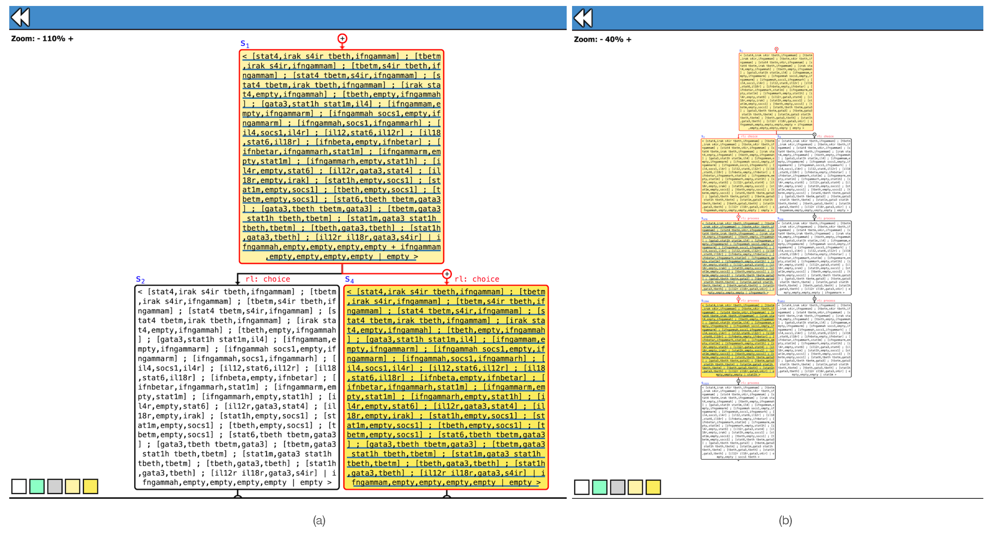In ANIMA, system biologists can explore the computation space of RSs in a stepwise manner by expanding state transitions one at a time with a simple point-and-click interface, thereby producing anincremental visual representation of the whole computation tree with regard to a given initial state. Let us see an example.

Example 9.

Consider the Maude encoding ${\mathcal{R}}_{{\mathcal{A}}_{GR}}$ of ${\mathcal{A}}_{GR}$ together with the following initial state:

$$\mathtt{init}=<\mathtt{GR}|\mathtt{ifngammah},\mathtt{empty},\mathtt{empty},\mathtt{empty},\mathtt{empty}+\mathtt{ifngammam},\mathtt{empty},\mathtt{empty},\mathtt{empty},\mathtt{empty}|\mathtt{empty}>$$

that includes two distinct context sequences, respectively, modeling a high gene expression level $\mathtt{ifngammah}$ and a medium gene expression level $\mathtt{ifngammam}$ in their initial contexts. By feeding  ANIMA  with ${\mathcal{R}}_{{\mathcal{A}}_{GR}}$ and $\mathtt{init}$, we can interactively generate the computation tree with regard to $\mathtt{init}$ by clicking on the node tree to be expanded. Figure 1a zooms into the first (non-deterministic) transition that applies the $\mathtt{choice}$ rule to select one of the two context sequences available in $\mathtt{init}$, while Figure 1b illustrates a partial expansion of the two possible evolutions of the system that depend on the chosen context sequence.

Note that the reader can fully reproduce this example by simply accessing  ANIMA  at the  http://safe-tools.dsic.upv.es/anima, (accessed on 14 March 2024) and selecting  Gene-Regulation-RS  from the list of pre-loaded examples.

As witnessed by Example 9, computations in a Maude specification ${\mathcal{R}}_{\mathcal{A}}$ can be textually large, hindering the comprehension and analysis of the reaction system behavior. The next section specifies a forward slicing technique that drastically reduces the complexity of system computations and facilitates the detection of causality relations in context-independent processes.

6. Forward Slicing of Context-Independent Processes

In this section, we present a forward slicing technique for context-independent processes. Although the generalization of the proposed slicing technique to generic interactive processes is not technically difficult, we prefer to focus on context-independent processes, since their behavior is totally defined by a single input context $C_0$ and having such a limited input allows one to precisely study the forward causalities of a reaction system. This approach is also advocated by [2], where a rigorous notion of minimal influence distance between entities is formalized within all possible context-independent state sequences.

Given a reaction system $\mathcal{A}=(S,A)$ and a context-independent process $\pi =(C_0,\delta )$ in $\mathcal{A}$, with $\delta =D_0,\dots ,D_n$, forward slicing aims at producing a partial view of $\pi$ that only depends on a selected subset $C_0^{\prime }$ of $C_0$ which is called slicing criterion. Forward slicing allows one to evaluate the impact of a set of input entities across the whole process, thereby giving answers to questions such as does the presence (or the absence) of an entity e in the slicing criterion affect the production of the entity $e^{\prime }$ in a later stage of π?

The forward slicing of context-independent processes can be specified by a rewrite theory ${\mathcal{R}}_{\mathcal{A}}^{▹}$ that slightly modifies and improves the Maude encoding ${\mathcal{R}}_{\mathcal{A}}$ of Section 4. ${\mathcal{R}}_{\mathcal{A}}^{▹}$ includes an extended version ${\mathcal{E}}_{\mathcal{A}}^{▹}$ of the equational theory ${\mathcal{E}}_{\mathcal{A}}$ that provides a richer algebraic data type for system states, as well as a new set of rewrite rules $R_{\mathcal{A}}^{▹}$ that implements an augmented reaction system semantics that models both a context-independent process and its sliced counterpart. We say that ${\mathcal{R}}_{\mathcal{A}}^{▹}$ is the forward slicing encoding for $\mathcal{A}$. In the following, we present the main data structures and core functions included in ${\mathcal{R}}_{\mathcal{A}}^{▹}$. The full specification is available at [16].

6.1. The Equational Theory ${\mathcal{E}}_{\mathcal{A}}^{▹}$

The code snippet in Listing 8 illustrates the key modifications introduced by ${\mathcal{E}}_{\mathcal{A}}^{▹}$, with respect to ${\mathcal{E}}_{\mathcal{A}}$.

Listing 8. Equational theory ${\mathcal{E}}_{\mathcal{A}}^{▹}$: main changes with regard to ${\mathcal{E}}_{\mathcal{A}}$.

1 sort Result .

2 op {_|_} : Reactions Entities -> Result .

3 vars A A’ : Reactions .

4 var Res : Result .

5 vars P P’ T : Entities .

6 op fail : -> Reaction .

7 op apply : Reaction Entities -> Reaction .

8 eq apply([R,I,P],T) = if en([ R,I,P],T) then [ R,I,P ] else fail fi .

9 op applyAll+ : Reactions Entities -> Result .

10 eq applyAll+(A,T) = $applyAll(A,T,{ empty | empty }) .

11 op $applyAll : Reactions Entities Result -> Result .

12 eq $applyAll(empty,T,Res) = Res .

13 eq $applyAll(([ R,I,P ] ; A), T , { A’ | P’ }) =

14          $applyAll(A, T, if apply([ R,I,P ],T) =/= fail  then

15                                   {[ R,I,P ] ; A’ | P P’}

16                            else

17                                   { A’ | P’ }

18                            fi

19                    ) .

20 op <_|_|_|_|_> : Reactions Entities Reactions Entities Reactions -> State .

21 op +<_|_> : Reactions Entities -> State .

22 op -<_|_> : Reactions Entities -> State .

Roughly speaking, ${\mathcal{E}}_{\mathcal{A}}^{▹}$ extends ${\mathcal{E}}_{\mathcal{A}}$ into two main directions.

Firstly, the function $\mathtt{applyAll}(\mathtt{A},\mathtt{T})$ in ${\mathcal{E}}_{\mathcal{A}}$, which computes the set of entities $re{s}_A\left(T\right)$, has been replaced by the function $\mathtt{applyAll}+(\mathtt{A},\mathtt{T})$ (see Lines 9–19 of Listing 8) whose resulting outcome is now a pair $\left\{{\mathtt{A}}^{\prime }\right|{\mathtt{T}}^{\prime }\}$ that keeps track of both the entities ${\mathtt{T}}^{\prime }$ produced by applying $\mathtt{A}$ on $\mathtt{T}$ and the sublist of reactions ${\mathtt{A}}^{\prime }$ which only includes the reactions of $\mathtt{A}$ that are enabled by $\mathtt{T}$ and thus are responsible for the production of ${\mathtt{T}}^{\prime }$. Note that, to implement this extension, we also need to slightly modify the function $\mathtt{apply}\left(\right[\mathtt{R},\mathtt{I},\mathtt{P}],\mathtt{T})$ (Lines 7–8), which now uses the special constant $\mathtt{fail}$ to explicitly signal that the reaction $[\mathtt{R},\mathtt{I},\mathtt{P}]$ cannot be applied to $\mathtt{T}$. Let us see an example.

Example 10.

Consider the RS ${\mathcal{A}}_{GR}=(S_{GR},A_{GR})$ of Example 6, whose reaction list is specified by the term $\mathtt{GR}$. The execution of the function call $\mathtt{applyAll}+(\mathtt{GR},\mathtt{stat}\mathtt{1}\mathtt{h}\mathtt{gata}\mathtt{3})$ yields the following outcome:

Maude> red applyAll+(GR,stat1h gata3) .

reduce in FORWARDSLICER-RS : applyAll+(GR, gata3 stat1h) .

rewrites: 341 in 0ms cpu (0ms real) (341000000 rewrites/second)

result Result: {[gata3,tbeth tbetm,gata3] ; [stat1h,empty,socs1] |

gata3 socs1}

which shows that only two reactions of $\mathtt{GR}$ (out of 32) are enabled by $\mathtt{stat}\mathtt{1}\mathtt{h}$ and $\mathtt{gata}\mathtt{3}$, thereby creating the new entities $\mathtt{gata}\mathtt{3}$ and $\mathtt{socs}\mathtt{1}$.

Secondly, ${\mathcal{E}}_{\mathcal{A}}^{▹}$ refines the notion of state, which we introduced in ${\mathcal{E}}_{\mathcal{A}}^{▹}$, by means of three novel operators (Lines 20–22) that allow system states to have multiple forms. A system state now can be

• A term of the form $<\mathtt{A}\left|\mathtt{D}\right|\mathtt{Au}|{\mathtt{D}}^{\prime }|{\mathtt{Au}}^{\prime }>$, where $\mathtt{A}$, $\mathtt{Au}$, ${\mathtt{Au}}^{\prime }$ are terms of sort $\mathtt{Reactions}$ and $\mathtt{D}$ and ${\mathtt{D}}^{\prime }$ are terms of sort $\mathtt{Entities}$. Intuitively, a state of this form stores the current configuration of a context-independent process together with its sliced counterpart. More formally, given a reaction list $\mathtt{A}$, $\mathtt{D}$ represents the entities which are currently present in the system, and $\mathtt{Au}$ is a list of reactions —included in $\mathtt{A}$— that have been used to produce $\mathtt{D}$. Similarly, ${\mathtt{D}}^{\prime }$ is the set of entities currently observed in the sliced counterpart that were produced by using the reactions in ${\mathtt{Au}}^{\prime }$.
• A term of the form $-<{\mathtt{A}}^{\prime }|{\mathtt{P}}^{\prime }>$, where ${\mathtt{A}}^{\prime }$ is a term of sort $\mathtt{Reactions}$ and ${\mathtt{P}}^{\prime }$ is a term of sort $\mathtt{Entities}$. This data structure is used to extract, from the current state, the entity set ${\mathtt{P}}^{\prime }$ of those entities that cannot be computed from the slicing criterion ${\mathtt{C}}_{\mathtt{0}}^{\prime }$ since the reactions in ${\mathtt{A}}^{\prime }$ did not take place. In other words, this state highlights the missing entities, that is, those entities that can be computed from the initial context ${\mathtt{C}}_{\mathtt{0}}$ but cannot be computed from the slicing criterion ${\mathtt{C}}_{\mathtt{0}}^{\prime }$.
• A term of the form $+<{\mathtt{A}}^{\prime }|{\mathtt{P}}^{\prime }>$, where ${\mathtt{A}}^{\prime }$ is a term of sort $\mathtt{Reactions}$ and ${\mathtt{P}}^{\prime }$ is a term of sort $\mathtt{Entities}$. This data structure is used to extract, from the current state, the entity set ${\mathtt{P}}^{\prime }$ of those entities that can be only computed from the slicing criterion ${\mathtt{C}}_{\mathtt{0}}^{\prime }$ since the reactions in ${\mathtt{A}}^{\prime }$ did not take place in the original process. Put differently, this state identifies the spurious entities, that is, those entities that can be computed from the slicing criterion ${\mathtt{C}}_{\mathtt{0}}^{\prime }$ but cannot be computed from the initial context ${\mathtt{C}}_{\mathtt{0}}$. Generation of spurious entities is typically caused by the absence of one or more inhibitors in ${\mathtt{C}}_{\mathtt{0}}^{\prime }$ that are instead present in ${\mathtt{C}}_{\mathtt{0}}$. This fact allows for a given reaction to take place in the sliced process, but it is blocked in the original process.

6.2. The Set of Rewrite Rules $R_{\mathcal{A}}^{▹}$

The forward slicing algorithm of context-independent processes is implemented by the three rewrite rules of Listing 9.

Listing 9. Rewrite rules of $R_{\mathcal{A}}^{▹}$.

1 vars D D’ D-new D-new’ : Entities .

2 vars A Au Au’ Au-new Au-new’ : Reactions .

3 crl [process-fs] : < A | D | Au | D’ | Au’ > =>

4                    < A | D-new | Au-new Au | D-new’ | Au-new’ Au’ > if

5                        { Au-new’ | D-new’ } := applyAll+(A,D’) /\

6                        { Au-new  | D-new } := applyAll+(A,D) .

7 rl [slice+] : < A | D | Au | D’ | Au’ > => +< (Au’ \ Au) | D’ \ D > .

8 rl [slice-] : < A | D | Au | D’ | Au’ > => -< (Au \ Au’) | D \ D’ > .

The process-fs rule is the backbone of the whole forward slicing algorithm. It allows the system to transition from a state

$$<\mathtt{A}|{\mathtt{D}}_{\mathtt{i}}|{\mathtt{Au}}_{\mathtt{i}}\left|{\mathtt{D}}_{\mathtt{i}}^{\prime }\right|{\mathtt{Au}}_{\mathtt{i}}^{\prime }>$$

to a state

$$<\mathtt{A}|{\mathtt{D}}_{\mathtt{i}+\mathtt{1}}|{\mathtt{Au}}_{\mathtt{i}+\mathtt{1}}\left|{\mathtt{D}}_{\mathtt{i}+\mathtt{1}}^{\prime }\right|{\mathtt{Au}}_{\mathtt{i}+\mathtt{1}}^{\prime }>$$

where

• $\mathtt{A}$ is a reaction list that models the reactions in the RS $\mathcal{A}=(S,A)$;
• ${\mathtt{D}}_{\mathtt{i}+\mathtt{1}}$ is a term encoding the set of entities obtained by applying the reaction list $\mathtt{A}$ on the set of entities encoded by ${\mathtt{D}}_{\mathtt{i}}$;
• ${\mathtt{Au}}_{\mathtt{i}+\mathtt{1}}$ is a reaction list that contains all and only the reactions used to produce ${\mathtt{D}}_{\mathtt{i}+\mathtt{1}}$;
• ${\mathtt{D}}_{\mathtt{i}+\mathtt{1}}^{\prime }$ is a term encoding the set of entities obtained by applying the reaction list $\mathtt{A}$ on the set of entities encoded by ${\mathtt{D}}_{\mathtt{i}}^{\prime }$;
• ${\mathtt{Au}}_{\mathtt{i}+\mathtt{1}}^{\prime }$ is a reaction list that contains all and only the reactions used to produce ${\mathtt{D}}_{\mathtt{i}+\mathtt{1}}^{\prime }$;

Note that the $\mathtt{process}‐\mathtt{fs}$ rule uses the function $\mathtt{applyAll}+$ to generate the entities and reactions at step $(i+1)$ by exploiting the information at step i.

In this scenario, all the computations of the form

$$<\mathtt{A}|{\mathtt{C}}_{\mathtt{0}}\left|\mathtt{empty}\right|{\mathtt{C}}_{\mathtt{0}}^{\prime }|\mathtt{empty}>{\stackrel{\mathtt{process}‐\mathtt{fs}}{⟶}}_{R_{\mathcal{A}}^{▹},{\mathcal{E}}_{\mathcal{A}}^{▹}}\dots {\stackrel{\mathtt{process}‐\mathtt{fs}}{⟶}}_{R_{\mathcal{A}}^{▹},{\mathcal{E}}_{\mathcal{A}}^{▹}}<\mathtt{A}|{\mathtt{D}}_{\mathtt{n}}|{\mathtt{A}}_{\mathtt{n}}\left|{\mathtt{D}}_{\mathtt{n}}^{\prime }\right|{\mathtt{A}}_{\mathtt{n}}^{\prime }>$$

define two context-independent processes in $\mathcal{A}$ that evolve concurrently: $\pi =(C_0,\delta )$, with $\delta =D_0,\dots ,D_n$ and ${\pi }^{\prime }=(C_0^{\prime },{\delta }^{\prime })$, with ${\delta }^{\prime }=D_0^{\prime },\dots ,D_n^{\prime }$. When $C_0^{\prime }\subseteq C_0$, we say that ${\pi }^{\prime }$ is a sliced version of $\pi$. Basically, a sliced version ${\pi }^{\prime }$ of $\pi$ encodes the behavior of an RS $\mathcal{A}$ on the reduced set of input entities specified by the slicing criterion $C_0^{\prime }$.

Proposition 2.

Let $\mathcal{A}=(S,A)$ be an RS and let ${\mathcal{R}}_{\mathcal{A}}^{▹}$ be the forward slicing encoding of $\mathcal{A}$. Let $C_0,C_0^{\prime }$ be two sets of entities such that $C_0^{\prime }\subseteq C_0$. Let ${\mathtt{C}}_{\mathtt{0}}$ and ${\mathtt{C}}_{\mathtt{0}}^{\prime }$ be two terms, respectively, encoding $C_0$ and $C_0^{\prime }$. If

$$\begin{array}{cc}\hfill <\mathtt{A}|{\mathtt{C}}_{\mathtt{0}}\left|\mathtt{empty}\right|{\mathtt{C}}_{\mathtt{0}}^{\prime }|\mathtt{empty}>& {\stackrel{\mathtt{process}‐\mathtt{fs}}{⟶}}_{R_{\mathcal{A}}^{▹},{\mathcal{E}}_{\mathcal{A}}^{▹}}<\mathtt{A}|{\mathtt{D}}_{\mathtt{1}}|{\mathtt{A}}_{\mathtt{1}}\left|{\mathtt{D}}_{\mathtt{1}}^{\prime }\right|{\mathtt{A}}_{\mathtt{1}}^{\prime }>\hfill \\ & ⋮\hfill \\ \hfill <\mathtt{A}|{\mathtt{D}}_{\mathtt{n}-\mathtt{1}}|{\mathtt{A}}_{\mathtt{n}-\mathtt{1}}\left|{\mathtt{D}}_{\mathtt{n}-\mathtt{1}}^{\prime }\right|{\mathtt{A}}_{\mathtt{n}-\mathtt{1}}^{\prime }>& {\stackrel{\mathtt{process}‐\mathtt{fs}}{⟶}}_{R_{\mathcal{A}}^{▹},{\mathcal{E}}_{\mathcal{A}}^{▹}}<\mathtt{A}|{\mathtt{D}}_{\mathtt{n}}|{\mathtt{A}}_{\mathtt{n}}\left|{\mathtt{D}}_{\mathtt{n}}^{\prime }\right|{\mathtt{A}}_{\mathtt{n}}^{\prime }>\hfill \end{array}$$

is a computation of length n in ${\mathcal{R}}_{\mathcal{A}}^{▹}$, $n\ge 0$, then there exist two n-step context-independent processes $\pi =(C_0,\delta )$, with $\delta =D_0,\dots ,D_n$ and ${\pi }^{\prime }=(C_0^{\prime },{\delta }^{\prime })$, with ${\delta }^{\prime }=D_0^{\prime },\dots ,D_n^{\prime }$ such that ${\mathtt{D}}_{\mathtt{0}},\dots ,{\mathtt{D}}_{\mathtt{n}}$ and ${\mathtt{D}}_{\mathtt{0}}^{\prime },\dots ,{\mathtt{D}}_{\mathtt{n}}^{\prime }$ are the terms encoding the result sequences $D_0,\dots ,D_n$ and $D_0^{\prime },\dots ,D_n^{\prime }$. and ${\pi }^{\prime }$ is a sliced version of π.

Proof. 

The proof is by induction on the length n of the computation

$$\begin{array}{cc}\hfill {\mathcal{C}}_n=<\mathtt{Rs}|{\mathtt{C}}_{\mathtt{0}}\left|\mathtt{empty}\right|{\mathtt{C}}_{\mathtt{0}}^{\prime }|\mathtt{empty}>& {\stackrel{\mathtt{process}‐\mathtt{fs}}{⟶}}_{R_{\mathcal{A}}^{▹},{\mathcal{E}}_{\mathcal{A}}^{▹}}<\mathtt{A}|{\mathtt{D}}_{\mathtt{1}}|{\mathtt{A}}_{\mathtt{1}}\left|{\mathtt{D}}_{\mathtt{1}}^{\prime }\right|{\mathtt{A}}_{\mathtt{1}}^{\prime }>\hfill \\ & ⋮\hfill \\ \hfill <\mathtt{A}|{\mathtt{D}}_{\mathtt{n}-\mathtt{1}}|{\mathtt{A}}_{\mathtt{n}-\mathtt{1}}\left|{\mathtt{D}}_{\mathtt{n}-\mathtt{1}}^{\prime }\right|{\mathtt{A}}_{\mathtt{n}-\mathtt{1}}^{\prime }>& {\stackrel{\mathtt{process}‐\mathtt{fs}}{⟶}}_{R_{\mathcal{A}}^{▹},{\mathcal{E}}_{\mathcal{A}}^{▹}}<\mathtt{A}|{\mathtt{D}}_{\mathtt{n}}|{\mathtt{A}}_{\mathtt{n}}\left|{\mathtt{D}}_{\mathtt{n}}^{\prime }\right|{\mathtt{A}}_{\mathtt{n}}^{\prime }>\hfill \end{array}$$

$n=0.$

This case is trivial. The computation ${\mathcal{C}}_0$ does not include any rewrite step and thus leaves the initial state $<\mathtt{Rs}|{\mathtt{C}}_{\mathtt{0}}\left|\mathtt{empty}\right|{\mathtt{C}}_{\mathtt{0}}^{\prime }|\mathtt{empty}>$ unchanged. Note that this state encodes two 0-step context-independent processes: ${\pi }_0=(C_0,{\delta }_0)$, with ${\delta }_0=D_0=\varnothing$ and ${\pi }_0^{\prime }=(C_0^{\prime },{\delta }_0^{\prime })$, with ${\delta }_0^{\prime }=D_0^{\prime }=\varnothing$.

$n>0.$

By inductive hypothesis, there is a computation of length $n-1$

$$\begin{array}{cc}\hfill {\mathcal{C}}_{n-1}=<\mathtt{Rs}|{\mathtt{C}}_{\mathtt{0}}\left|\mathtt{empty}\right|{\mathtt{C}}_{\mathtt{0}}^{\prime }|\mathtt{empty}>& {\stackrel{\mathtt{process}‐\mathtt{fs}}{⟶}}_{R_{\mathcal{A}}^{▹},{\mathcal{E}}_{\mathcal{A}}^{▹}}<\mathtt{A}|{\mathtt{D}}_{\mathtt{1}}|{\mathtt{A}}_{\mathtt{1}}\left|{\mathtt{D}}_{\mathtt{1}}^{\prime }\right|{\mathtt{A}}_{\mathtt{1}}^{\prime }>\hfill \\ & ⋮\hfill \\ \hfill <\mathtt{A}|{\mathtt{D}}_{\mathtt{n}-\mathtt{2}}|{\mathtt{A}}_{\mathtt{n}-\mathtt{2}}\left|{\mathtt{D}}_{\mathtt{n}-\mathtt{2}}^{\prime }\right|{\mathtt{A}}_{\mathtt{n}-\mathtt{2}}^{\prime }>& {\stackrel{\mathtt{process}‐\mathtt{fs}}{⟶}}_{R_{\mathcal{A}}^{▹},{\mathcal{E}}_{\mathcal{A}}^{▹}}<\mathtt{A}|{\mathtt{D}}_{\mathtt{n}-\mathtt{1}}|{\mathtt{A}}_{\mathtt{n}-\mathtt{1}}\left|{\mathtt{D}}_{\mathtt{n}-\mathtt{1}}^{\prime }\right|{\mathtt{A}}_{\mathtt{n}-\mathtt{1}}^{\prime }>\hfill \end{array}$$

such that there exist two $(n-1)$-step context-independent processes ${\pi }_{n-1}=(C_0,{\delta }_{n-1})$, with $\delta =D_0,\dots ,D_{n-1}$, and ${\pi }_{n-1}^{\prime }=(C_0^{\prime },{\delta }_{n-1}^{\prime })$, with ${\delta }^{\prime }=D_0^{\prime },\dots ,D_{n-1}^{\prime }$, where ${\mathtt{D}}_{\mathtt{0}},\dots ,{\mathtt{D}}_{\mathtt{n}-\mathtt{1}}$, and ${\mathtt{D}}_{\mathtt{0}}^{\prime },\dots ,{\mathtt{D}}_{\mathtt{n}-\mathtt{1}}^{\prime }$ are the terms that encode the result sequences $D_0,\dots ,$$D_{n-1}$ and $D_0^{\prime },\dots ,D_{n-1}^{\prime }$, respectively. Furthermore, ${\pi }_{n-1}^{\prime }$ is a sliced version of ${\pi }_{n-1}$.

Observe also that it is always possible to perform the rewrite step

$$r=<\mathtt{A}|{\mathtt{D}}_{\mathtt{n}-\mathtt{1}}|{\mathtt{A}}_{\mathtt{n}-\mathtt{1}}|{\mathtt{D}}_{\mathtt{n}-\mathtt{1}}^{\prime }|{\mathtt{A}}_{\mathtt{n}-\mathtt{1}}^{\prime }>{\stackrel{\mathtt{process}‐\mathtt{fs}}{⟶}}_{R_{\mathcal{A}}^{▹},{\mathcal{E}}_{\mathcal{A}}^{▹}}<\mathtt{A}|{\mathtt{D}}_{\mathtt{n}}|{\mathtt{A}}_{\mathtt{n}}\left|{\mathtt{D}}_{\mathtt{n}}^{\prime }\right|{\mathtt{A}}_{\mathtt{n}}^{\prime }>$$

which uses the function applyAll+ to generate ${\mathtt{D}}_{\mathtt{n}}$ and ${\mathtt{D}}_{\mathtt{n}}^{\prime }$ from ${\mathtt{D}}_{\mathtt{n}-\mathtt{1}}$ and ${\mathtt{D}}_{\mathtt{n}-\mathtt{1}}^{\prime }$. Since ${\mathtt{D}}_{\mathtt{n}-\mathtt{1}}$ and ${\mathtt{D}}_{\mathtt{n}-\mathtt{1}}^{\prime }$ are the terms encoding the set of entities $D_{n-1}$ and $D_{n-1}^{\prime }$, we have that ${\mathtt{D}}_{\mathtt{n}}$ and ${\mathtt{D}}_{\mathtt{n}}^{\prime }$ are the terms encoding the set of entities $D_n$ and $D_n^{\prime }$. Therefore, to prove the proposition, it suffices to consider the computation ${\mathcal{C}}_n$ of length n that concatenates the computation ${\mathcal{C}}_{n-1}$ with the rewrite step r. □

While the process-fs rule formalizes system progress in ${\mathcal{R}}_{\mathcal{A}}^{▹}$, the $\mathtt{slice}-$ and $\mathtt{slice}+$ rules extract specific pieces of information from a given computation state $\mathtt{st}$ that allow for the original process $\pi$ and its sliced counterpart ${\pi }^{\prime }$ to be compared on $\mathtt{st}$.

More precisely, given a state $\mathtt{st}=<\mathtt{A}|{\mathtt{D}}_{\mathtt{i}}|{\mathtt{A}}_{\mathtt{i}}\left|{\mathtt{D}}_{\mathtt{i}}^{\prime }\right|{\mathtt{A}}_{\mathtt{i}}^{\prime }>$, the $\mathtt{slice}-$ rule uses the set difference operator (To be more precise, ∖ is an overloaded operator that can be applied to both entity sets and reaction lists.)\ to compute the new state $-<({\mathtt{A}}_{\mathtt{i}}$\${\mathtt{A}}_{\mathtt{i}}^{\prime }\left)\right|{\mathtt{D}}_{\mathtt{i}}$\${\mathtt{D}}_{\mathtt{i}}^{\prime }>$ that isolates

• The entities $({\mathtt{D}}_{\mathtt{i}}$\${\mathtt{D}}_{\mathtt{i}}^{\prime })$ in $\mathtt{st}$ that can be computed in (the i-th step of) $\pi$ but not in (the i-th step of) ${\pi }^{\prime }$.
• The reactions $({\mathtt{A}}_{\mathtt{i}}$\${\mathtt{A}}_{\mathtt{i}}^{\prime })$ in $\mathtt{st}$ that were enabled in $\pi$ but not in ${\pi }^{\prime }$ until the i-th step.

Note that $({\mathtt{A}}_{\mathtt{i}}$\${\mathtt{A}}_{\mathtt{i}}^{\prime })$ represents the reason of the missing information $({\mathtt{D}}_{\mathtt{i}}$\${\mathtt{D}}_{\mathtt{i}}^{\prime })$: in other words, entities encoded by $({\mathtt{D}}_{\mathtt{i}}$\${\mathtt{D}}_{\mathtt{i}}^{\prime })$ cannot be produced in the i-th step of ${\pi }^{\prime }$ because reactions $({\mathtt{A}}_{\mathtt{i}}$\${\mathtt{A}}_{\mathtt{i}}^{\prime })$ were never enabled in ${\pi }^{\prime }$ up to the i-th step.

Dually, the $\mathtt{slice}+$ computes the new state $+<({\mathtt{A}}_{\mathtt{i}}^{\prime }$\${\mathtt{A}}_{\mathtt{i}}\left)\right|{\mathtt{D}}_{\mathtt{i}}^{\prime }$\${\mathtt{D}}_{\mathtt{i}}>$ that isolates:

• The entities $({\mathtt{D}}_{\mathtt{i}}^{\prime }$\${\mathtt{D}}_{\mathtt{i}})$ in $\mathtt{st}$ that can be computed in (the i-th step of) ${\pi }^{\prime }$ but not in (the i-th step of) $\pi$.
• The reactions $({\mathtt{A}}_{\mathtt{i}}^{\prime }$\${\mathtt{A}}_{\mathtt{i}})$ in $\mathtt{st}$ that were enabled in ${\pi }^{\prime }$ but not in $\pi$ until the i-th step.

Intuitively, $\mathtt{slice}+$ collects the spurious entities $({\mathtt{D}}_{\mathtt{i}}^{\prime }$\${\mathtt{D}}_{\mathtt{i}})$ of $\mathtt{st}$, that is, those entities of $\mathtt{st}$ computed in ${\pi }^{\prime }$ by using the reactions $({\mathtt{A}}_{\mathtt{i}}^{\prime }$\${\mathtt{A}}_{\mathtt{i}})$ that are not enabled in $\pi$ (up to the i-th step).

It is worth noting that, all the three rules process-fs, $\mathtt{slice}-$, and $\mathtt{slice}+$ can be non-deterministically applied to each system state. Therefore, at each state, the system can (i) evolve via the process-fs rule, (ii) compute the missing entities in ${\pi }^{\prime }$ by applying $\mathtt{slice}-$, or (iii) compute the spurious entities by applying $\mathtt{slice}+$. Let us see an example.

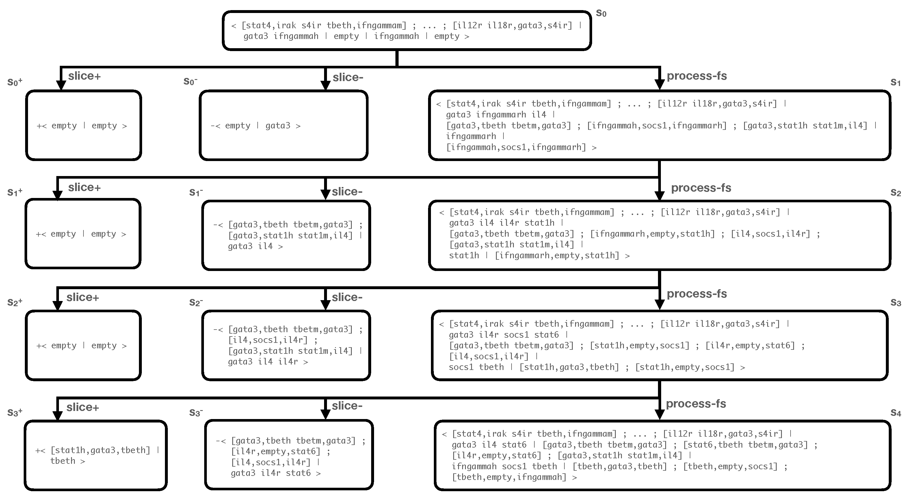
Example 11.

Let ${\mathcal{A}}_{GR}=(S_{GR},A_{GR})$ be the RS of Example 6. Let $C_0=\{\mathit{ifngammh},gata3\}$ be an initial context and let $C_0^{\prime }=\left\{\mathit{ifngammah}\right\}$ be a slicing criterion for $C_0$. Given the initial state

$$\mathtt{init}=<\mathtt{GR}|{\mathtt{C}}_{\mathtt{0}}\left|\mathtt{empty}\right|{\mathtt{C}}_{\mathtt{0}}^{\prime }|\mathtt{empty}>$$

where $\mathtt{GR}$ is the reaction list encoding the 32 reactions in $A_{GR}$, ${\mathtt{C}}_{\mathtt{0}}$ and ${\mathtt{C}}_{\mathtt{0}}^{\prime }$ are terms encoding $C_0$ and $C_0^{\prime }$, the (fragment of the) computation tree $T_{{\mathcal{R}}_{{\mathcal{A}}_{GR}}^{▹}}\left(\mathtt{init}\right)$ of Figure 2 can be computed in ${\mathcal{R}}_{{\mathcal{A}}_{GR}}^{▹}$. Note that each tree level $\mathtt{i}$ (except for the root level) contains three states:

(i) 

The current state ${\mathtt{s}}_{\mathtt{i}}$ which is produced by the application of the  process-fs  rule on the previous state ${\mathtt{s}}_{(\mathtt{i}-\mathtt{1})}$;

(ii) 

Two states ${\mathtt{s}}_{{(\mathtt{i}-\mathtt{1})}^{-}}$ and ${\mathtt{s}}_{{(\mathtt{i}-\mathtt{1})}^{+}}$ that specify the states which are computed by, respectively, applying the  slice-  and  slice+  rules to the state ${\mathtt{s}}_{(\mathtt{i}-\mathtt{1})}$.

Compact state views, which are produced by  slice-  and  slice+, allow one to immediately grasp what is going on in the process and its sliced counterpart.

For instance, by inspecting all the applications of  slice+  in the tree, we can immediately note that only state ${\mathtt{s}}_{\mathtt{3}}$ introduces a spurious entity (up to level 3); concretely, the entity  tbeth  which appears in the state

s₃₊ = +< [stat1h,gata3,tbeth] | tbeth >

Hence, we can infer that the gene expression $\mathit{tbeth}$ can be computed for the slicing criterion $C_0^{\prime }$ but not for the full initial context $C_0$ in the considered tree fragment. Indeed, the reaction  [stat1h,gata3,tbeth], which occurs in ${\mathtt{s}}_{{\mathtt{3}}^{+}}$, is enabled in the sliced process ${\pi }^{\prime }$ but not in the original one π. Since $\mathit{gata}\mathit{3}$ belongs to $C_0$ but not to $C_0^{\prime }$, we can safely say that $\mathit{gata}\mathit{3}$ blocks the creation of $\mathit{tbeth}$ in π.

Also, by looking at the applications of the  slice-  rule, we can easily detect the information that the slicing criterion $C_0^{\prime }$ cannot produce for a given computation state. For example, the state ${\mathtt{s}}_{{\mathtt{3}}^{-}}$ tells us that $\mathit{gata}\mathit{3}$, $\mathit{il}\mathit{4}\mathit{r}$, and $\mathit{stat}\mathit{6}$ are missing entities that cannot be created in the sliced process ${\pi }^{\prime }$ that reaches state ${\mathtt{s}}_{\mathtt{3}}$. This is due to the fact that reactions  [gata3,tbeth tbetm,gata3],  [il4r,empty,stat6], and  [il4,socs1,il4r]  take place only in π but not in ${\pi }^{\prime }$.

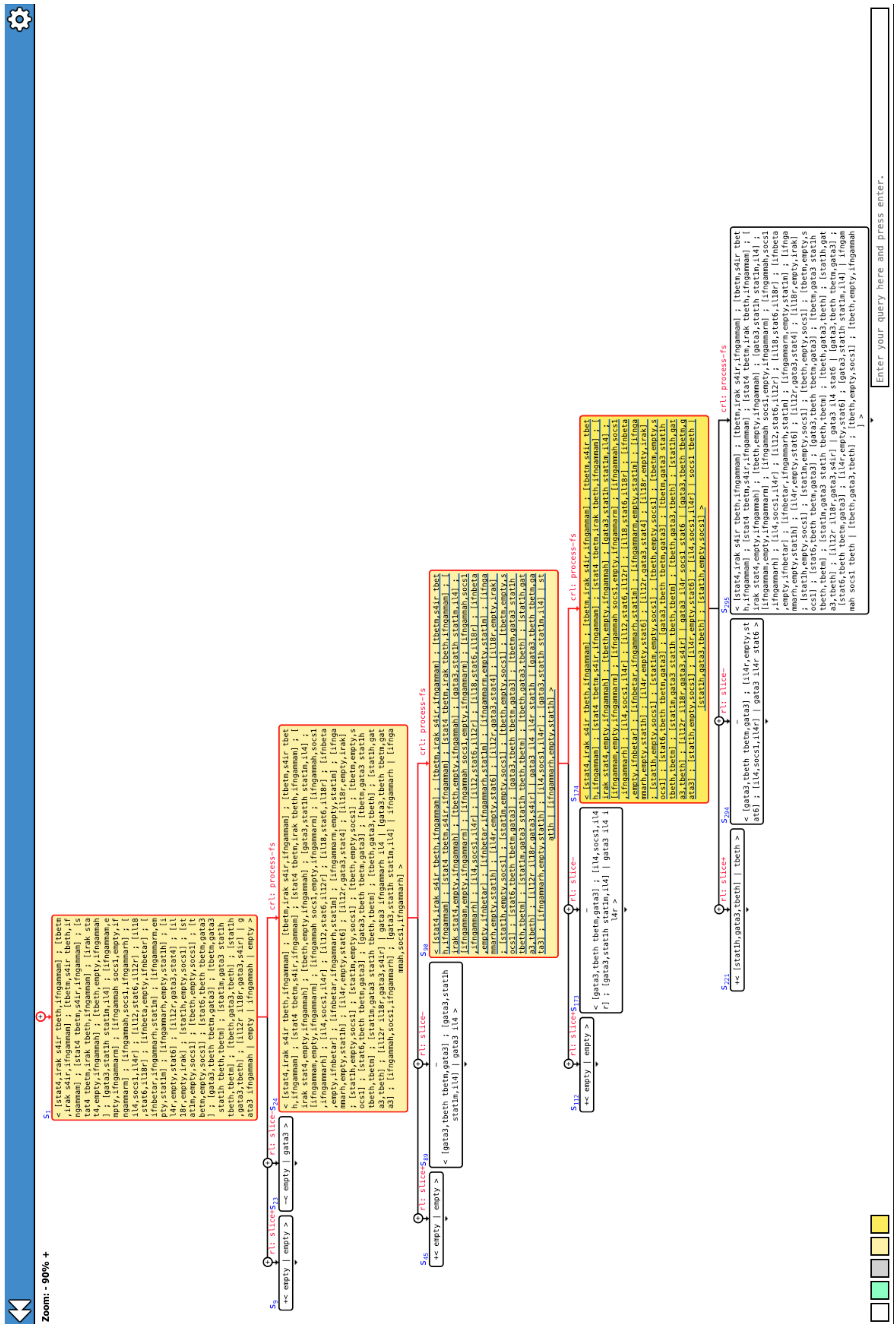
Finally, note that theANIMAsystem, which we presented in Section 5, can also be used to interactively execute the proposed forward slicing algorithm, allowing system biologists to visually explore system states and their associated compact views in a more user-friendly and incremental way. In this regard, Figure 3 illustrates the generation of the computation tree of Figure 2 withinANIMA. To reproduce this experiment, the reader can accessANIMAat thehttp://safe-tools.dsic.upv.es/anima(accessed on 14 March 2024) and select Forward Slicing of Gene-Regulation-RS from the list of pre-loaded examples.

Figure 2. Fragment of the computation tree $T_{{\mathcal{R}}_{{\mathcal{A}}_{GR}}^{▹}}\left(\mathtt{init}\right)$.

Figure 2. Fragment of the computation tree $T_{{\mathcal{R}}_{{\mathcal{A}}_{GR}}^{▹}}\left(\mathtt{init}\right)$.

Figure 3. Forward slicing of context-independent processes in ANIMA.

Figure 3. Forward slicing of context-independent processes in ANIMA.

7. Related Work

Several tools are already available to simulate RSs or to verify that certain properties are met. In [18,19], some authors developed BioReSolve [20]: a PROLOG interpreter for reaction system analysis. The verification capabilities integrated into BioReSolve have been crafted from scratch. In contrast, our approach offers a rewriting-based modeling of RSs, leveraging the extensive functionalities of the Maude environment, which provides multiple built-in functions and third-party tools for program analysis. Other implementations of RSs include brsim [21], a Basic Reaction System Simulator written in Haskell and distributed under the terms of GNU GPLv3 license [22] whose online version WEBRSIM makes all the features of brsim available through a friendly web interface [23]; HERESY [24], a GPU-based Highly Efficient REaction SYstem simulator, that exploits the large number of computational units inside GPUs to boost performance [25]; cl-rs [26], an optimised Common Lisp simulator for RSs presented in [27].

Model checking has been deeply studied in the context of reaction systems. [28] defines rsCTL, a temporal logic for reaction systems. The logic is interpreted over the models for the context-restricted reaction systems that generalize standard reaction systems by controlling context sequences. In [29,30], a variant of Linear Time Temporal Logic that is interpreted over models of reaction systems with discrete concentrations is presented: the approach adopts a suitable encoding in SMT together with bounded model checking for the formal verification of temporal properties over RSs. The verification technique has been implemented into the ReactICS system [31]. A more theoretical work that investigates model checking of reaction systems through computational complexity lenses is also presented in [32]. This work provides several complexity results for decision procedures related to properties of central interest in biomodeling (e.g., mass conservation, steady states, stationary processes).

We believe that model-checking and (trace and program) slicing may be successfully combined together to improve the analysis and comprehension of counter-examples generated by model-checkers when properties of interest are refuted.

Notably, the Maude language has already been successfully used in the analysis of biological systems. For instance, Pathway Logic [33] is a symbolic approach to the modeling and analysis of biological systems that is implemented in Maude. This logical framework allow metabolic pathways to be simulated and formally verified.

Dynamic program slicing has been applied previously to other programming paradigms, such as imperative programming [8], functional programming [34], and term rewriting and its extensions [35,36]. None of these approaches are suitable for RSs, which have a completely different computation behavior based on the non-monotonic enabling mechanism of reactions. In [37], we extended BioReSolve with a slicing algorithm which proceeds backwards. Some entities in the last state of a computation of an RS are selected and then the algorithm proceeds backwards, simplifying the computation and leaving only the entities which are essential to derive the selected ones. Unfortunately, this way we cannot know in advance which entities of the initial state of the computation will be left in the backward sliced computation. In this paper, we define a dual forward slicing algorithm in which we observe some entities in the initial state and we proceed forward. The two (backward and forward) slicing methodologies clearly derive different information as they focus on input information from different states and apply different algorithms. While the forward slicing results in a form of impact analysis that identifies the scope and potential consequences of changing the program input, backward slicing allows for provenance analysis to be performed in search of the origins of the selected entities.

8. Conclusions and Future Work

In this paper, we have defined the first implementation of reaction systems in Maude, a language based on rewriting logic, which has a very well-developed environment with tools for program analysis and verification. Our Maude implementation provides an interpreter for RSs that supports exploration capabilities via Maude built-in commands as well as third-party systems such as the ANIMA system. Also, we have defined an algorithm for forward slicing of context-independent processes. Our implementation of forward slicing gives a parallel execution of the standard and the sliced computation, so that users can compare each state of the original computation with the corresponding sliced one, and obtain useful information to analyze and possibly debug RS processes. To evaluate the feasibility and usefulness of the proposed approach, our forward slicing algorithm has been used to analyze an example of a gene regulatory network.

As future work, we want to study the combination of the forward slicing algorithm with the backward one which we have defined in [37]. We believe that this integration can improve the quality of the analysis, allowing for more erroneous/unexpected behaviours to be detected. We also want to extend the forward slicing algorithm to a language for concurrent multiparty communications [38], and investigate possible extensions that exploit static analysis techniques [39,40,41] as well as dynamic verification methodologies [42,43].