A Reactive Deep Learning-Based Model for Quality Assessment in Airport Video Surveillance Systems

Abstract

Monitoring the correct operation of airport video surveillance systems is of great importance in terms of the image quality provided by the cameras. Performing this task using human resources is time-consuming and usually associated with a delay in diagnosis. For this reason, in this article, an automatic system for image quality assessment (IQA) in airport surveillance systems using deep learning techniques is presented. The proposed method monitors the video surveillance system based on the two goals of “quality assessment” and “anomaly detection in images”. This model uses a 3D convolutional neural network (CNN) for detecting anomalies such as jitter, occlusion, and malfunction in frame sequences. Also, the feature maps of this 3D CNN are concatenated with feature maps of a separate 2D CNN for image quality assessment. This combination can be useful in improving the concurrence of correlation coefficients for IQA. The performance of the proposed model was evaluated both in terms of quality assessment and anomaly detection. The results show that the proposed 3D CNN model could correctly detect anomalies in surveillance videos with an average accuracy of 96.48% which is at least 3.39% higher than the compared methods. Also, the proposed hybrid CNN model could assess image quality with an average correlation of 0.9014, which proves the efficiency of the proposed method.

1. Introduction

An airport terminal monitoring system comprises a digital distributed network infrastructure, encompassing management servers, storage servers, digital cameras, and other essential equipment [1]. At present, the monitoring and management systems used in the airports can realize the monitoring of video loss, disconnection of encoder equipment, server failure, hard disk failure, and other equipment status, but cannot realize the monitoring of some soft faults such as video image quality problems [2,3]. Because the network digital camera in the video acquisition, coding, transmission and decoding, and other conventional video information processing processes, often produces video data damage, resulting in video image quality decline, hindering people from obtaining information from the video image, serious distortion will also affect the monitoring effect, resulting in monitoring failure [4]. The soft failure of the system caused by video quality is the main component of the system failure, which will also have a bad impact on the normal use of the system and reduce the efficiency of airport air defense security [5]. However, in terms of surveillance video quality monitoring, airport operation and maintenance personnel still use manual inspection. With the increasing number of terminal surveillance cameras and the continuous improvement in surveillance video quality requirements, the traditional manual inspection method has several disadvantages.

In addition to being time-consuming, laborious, and inefficient, manual inspection is not good in terms of failure response speed, and surveillance video signals in various failures often cannot be found in time by operation and maintenance personnel, which results in a loss of data or loss of video quality [6]. Also, manual inspection has certain limitations and instabilities caused by people’s lack of concentration, fatigue or other factors, so that such manual inspection results are not objective [7]. On the other hand, due to the limited number of displays, maintenance personnel often monitor multiple cameras at the same time in a monitor screen or randomly extract the camera display, resulting in some monitoring points being missed or ignored [8].

In the face of thousands of front-end cameras, the operation and maintenance mode of manual video quality analysis and detection has long been difficult to sustain, and manual maintenance generally adopts periodic sampling inspection, which makes it difficult to achieve the purpose of 24 h real-time monitoring [9]. Therefore, to improve the inspection efficiency of the monitoring system and realize real-time monitoring of monitoring quality, it is of great significance to design a system based on video image quality assessment.

The mentioned challenges in the manual inspection of airport video surveillance systems have motivated the current research. The main objective of this research is to design a video quality assessment system based on video analysis technology to achieve real-time monitoring of security monitoring in airport areas, which can evaluate the quality of a surveillance video and automatically record it in the database for later statistics and queries. This research separates this main objective into two minor goals. First, to introduce an automatic model for detecting anomalies such as malfunctioning, jitter or malicious occlusion in videos. Second, to describe the quality of recorded videos as a quantitative metric. The strategies resulting from the fulfillment of these two goals are utilized for the formation of a warning system that is activated in case of anomaly/quality degrading detection in surveillance videos. The current research uses a combination of deep learning models to meet the mentioned goals. In the proposed method, a new combination of CNN models is presented for detecting anomalies and assessing the quality of monitoring data simultaneously. This model includes a 3D CNN for detecting anomalies in video frame sequences. In the proposed hybrid model, the concatenation of feature maps of the aforementioned 3D CNN model with a 2D CNN model is used for video quality assessment. In the architecture of these CNN models, hybrid pooling layers are used, based on which the generality of learning models can be improved. The contributions of this paper is twofold: First, this paper presents a new 3D CNN model based on hybrid pooing layers for detecting anomalies in airport video surveillance systems. Second, this article presents a novel parallel model based on 2D and 3D CNNs for quality assessment in airport video surveillance systems. The remainder of this section is dedicated to review of the related works.

1.1. Related Works

The current research includes the two research fields of image quality assessment and video anomaly detection. Each of these research fields includes a detailed background, and we will continue to review some of the recent efforts in each one.

1.1.1. Image Quality Assessment

Image quality assessment involves extracting features related to image quality through subjective and objective means, and then assessing the degree of image distortion using statistical learning techniques. There are two types of evaluation methods: subjective and objective. Subjective evaluation involves a group of raters assessing image quality, usually represented by mean opinion score (MOS) or difference mean opinion score (DMOS) [10]. MOS normalizes observer scores, while DMOS normalizes scores based on the difference between undistorted and distorted images.

Due to the impracticality and heavy workload of subjective evaluation, objective image quality evaluation algorithms are more suitable for practical problems. The objective evaluation method involves the computer calculating the quality index of the image using algorithms. However, different objective evaluation indicators can differ significantly from subjective perceptions.

Objective evaluation indexes can be divided into three types based on the presence of reference image information when predicting distorted image quality: full reference (FR), reduced reference (RR), and no reference (NR) image quality evaluation methods [11]. FR-IQA, which focuses on full-reference image quality evaluation, has seen significant advancements with the emergence of influential algorithms. Traditional algorithms like the Peak-Signal-to-Noise Ratio (PSNR) are commonly used to evaluate image quality after compression compared to the original image [12]. PSNR measures the distortion after compression, with higher values indicating lower distortion. While PSNR is widely used, it has limitations, such as being highly influenced by pixels, low consistency with subjective evaluation, and not considering important characteristics of the Human Visual System (HVS).

To address these limitations, evaluation methods based on the HVS have been proposed, such as error sensitivity analysis and the Structural Similarity Index (SSIM) [12]. SSIM assumes that HVS can extract structural information from the scene independently of local brightness and contrast. Improved FR algorithms based on SSIM, such as FSIM and FSIMc, have been developed by incorporating color feature measures, weighted averages, and phase consistency information. The Multi-Scale Structural Similarity Index (MS-SSIM) [12] and Information Content Weighted Structural Similarity Index (IW-SSIM) [13] have also been introduced, combining image details at different resolutions and observation conditions into quality assessment algorithms. Overall, FR-IQA algorithms are continuously improving in terms of performance, speed, and accuracy.

For situations where obtaining a reference image is not possible, such as in many practical applications, the semi-reference image quality evaluation method (RR-IQA) has been developed. Although the full reference image quality evaluation method has shown good results, RR-IQA only requires partial information or indirect features of the reference image. Maalouf et al. [14] proposed an RR algorithm based on group transformation, which extracts texture and gradient information from the reference and distorted images using an image group. The information is then processed through CSF filtering and threshold value to obtain the sensitivity coefficient, which is used to estimate the image quality by comparing the sensitivity coefficient of the distorted image with that of the reference image. Omari et al. [15] proposed an RR-IQA algorithm that operates on blocked or blurred degraded images by using local harmonic analysis to detect images from the edge and calculate local harmonic amplitude information. This information is then used with the distorted images to estimate image quality. Other RR-IQA methods are based on Natural Scene Statistics (NSS).

Typically, image quality assessment (IQA) methods require reference images for accurate evaluation, which yields good results. However, in practical scenarios, reference images are often unavailable or too expensive, making the task of no reference image quality evaluation (NR-IQA) more meaningful. NR-IQA algorithms mainly focus on detecting specific types of distortion like blur, block effects, and various forms of noise. For instance, algorithms estimating sharpness and blur have shown effectiveness in evaluating the quality of fuzzy images. NR-IQA methods can assess the degree of blur in an image, employing edge analysis techniques such as Sobel and Canny for extracting image edges. SVM-based methods are also utilized, where features from the spatial or transform domain are extracted and a Support Vector Regression (SVR) model is trained based on existing data, or an SVM + SVR model is used for distorted images. Representative algorithms in this context include BIQI, DIIVINE, BiQI, and SVR. Gupta et al. [16] introduced the DIIVINE algorithm, which employs controllable pyramid wavelet decomposition to extract statistical features from normalized wavelet coefficients and establish regression models. Mittal et al. [17] proposed the BRISQUE algorithm, which builds a regression model by extracting statistical features from the spatial normalization coefficient of images. However, the estimation effect of the quality score is not superior to that of the best blind degradation type method. Alternatively, probabilistic models like BLIINDS [18] and NIQE, as well as codebook-based methods like CORNIA [12], have been used. Additionally, CORNIA demonstrated that image features can be directly learned from the original image pixels, eliminating the need for manual extraction.

In recent years, the field of image quality evaluation has witnessed the emergence of deep learning-based algorithms. Deep learning, particularly Convolutional Neural Networks (CNNs), has demonstrated remarkable performance in various image processing tasks. The deep structure of CNNs enables the effective learning of complex mappings between input and output. One notable advantage of CNNs is their ability to directly take the original image as input and incorporate feature learning into the training process. This deep structure allows for efficient learning of complex mappings while requiring minimal domain knowledge.

Researchers, such as Kang et al. [19], have successfully utilized CNNs to accurately predict no reference image quality assessment (NR-IQA). Their approach involved a five-layer CNN model consisting of convolution, max–min pooling, and fully connected layers. By using overlapped sampled image blocks as input, the network model extracted relevant features from the corresponding spatial domain and predicted the quality fraction of the image blocks. This integrated approach of feature learning and regression in the optimization process resulted in a more efficient model for estimating image quality. The method demonstrated superior performance on LIVE datasets and exhibited excellent generalization ability in cross-dataset experiments. Additionally, local distortion experiments were conducted to validate the CNN’s local quality estimation ability.

Another deep learning-based approach, introduced by Gu et al. [20], is the Deep learning-based Image Quality Index (DIQI). In this method, the RGB image is converted to the YIQ color space, and 3000 features are extracted. A sparse auto-encoder is then trained using the L-BFGS algorithm. The input data are represented as a matrix of s × 3000, where s denotes the number of training samples. The output is calculated using a linear function, and the weights of each DNN layer are fine-tuned based on the loss function using a backpropagation algorithm. Experimental results have demonstrated the effectiveness of DIQI, and when compared to classical Full Reference (FR) and Reduced Reference (RR) IQA algorithms, it showcased the promising potential of DNN in IQA research.

Liu et al. [21] introduced the RankIQA model for evaluating the quality of unreferenced images. Unlike previous models that focused on feature extraction and network improvements, RankIQA addresses the issue of limited image datasets. It achieves this by employing data preprocessing techniques to generate distorted images of various levels and ordering types from known quality images. The model utilizes a weight-sharing network to sort images based on their quality using the generated sorted image set. Subsequently, the entire network is fine-tuned, and the trained network is transformed into a traditional convolutional neural network to estimate the image quality score from a single image. The authors propose an efficient backpropagation method in the weight-sharing network, which exhibits faster convergence and lower loss compared to standard pairwise and hard negative sampling. Experimental results on the TID2013 dataset demonstrate that RankIQA surpasses state-of-the-art methods by 5%. Additionally, in the LIVE dataset, RankIQA outperforms existing NR-IQA techniques and even the latest FR-IQA techniques, highlighting its ability to infer image quality without reference images.

In [22,23], researchers propose deep learning approaches for blind image quality assessment that achieve state-of-the-art performance in both synthetic and authentic distortion scenarios. In [22], a deep bilinear model called DB-CNN is introduced, consisting of two streams of CNNs specialized in different distortion scenarios. For synthetic distortions, the model pre-trains a CNN to classify the type and level of distortion in an input image. For authentic distortions, a pre-trained VGG-16 CNN is used for image classification. The features from the two streams are bilinearly pooled to obtain a final quality prediction. The model is fine-tuned on target databases using a variant of stochastic gradient descent. In [23], a Distortion Graph Representation (DGR) learning framework named LIQA is proposed. Each distortion is represented as a graph within this framework. It includes two sub-networks: Type Discrimination Network (TDN) and the Fuzzy Prediction Network (FPN). TDN aims to embed the DGR into a compact code to better discriminate distortion types and learn the relationships between them. FPN, on the other hand, extracts the distributional characteristics of the samples in a DGR and predicts fuzzy degrees based on a Gaussian prior.

1.1.2. Video Anomaly Detection

Anomaly detection in video surveillance systems may include tasks such as detecting video jitter, occlusion, anomaly in lighting, unauthorized objects and so on. This section reviews some of the efforts for each task.

A.

Video jitter detection

Video jitter is characterized by an overall displacement between frames, making the detection of this displacement crucial in identifying jitter. Various methods are commonly used for displacement estimation, including the optical flow method [24], block matching method, feature point matching method, and gray projection method [25]. The optical flow method utilizes fast corner detection and LK sparse optical flow. However, it heavily relies on the detection of feature points, which can lead to inaccurate results when there are limited corner points in the current environment. Additionally, obtaining better results requires a larger computational effort. Furthermore, the optical flow method is prone to producing incorrect estimates of moving objects in real-world environments, making it less robust [24]. The feature point matching method is more dependent on the search for feature points compared to the optical flow method. This often requires a significant computational load to find more accurate feature points, resulting in slower processing speeds. On the other hand, the gray projection method is commonly used due to its relatively lower computational requirements and better overall performance. Therefore, it is a viable option for practical applications [25].

B.

Surveillance video occlusion

At present, the occlusion boundary detection methods based on video sequences fall into two categories [26]: motion analysis-based models and machine learning-based models. The motion analysis-based models only use motion estimation to determine the occlusion boundary, but any error in the motion vector field may cause a high error in detecting the occlusion boundary, and the generality of this method is poor [27]. To overcome the shortcomings of motion analysis-based methods, some scholars have proposed a machine learning-based occlusion boundary detection. The most representative is Stein’s occlusion detection model, which uses supervised learning, is based on multiple color images, and completes occlusion boundary detection by combining motion cues and local edge cues. It can be seen from the analysis that the occlusion boundary detection method based on the idea of supervised learning can solve the existing problems in the motion analysis method to a certain extent [28]. However, in many practical problems, although a large amount of data can be easily obtained, it requires high material resources and manpower to mark these data, and in some cases, it is impossible to complete the data marking. As a result, supervised learning is not possible. The phenomenon of less labeled data and more unlabeled data is more obvious in online applications. Given this, scholars also put forward the occlusion boundary detection method based on unsupervised online learning [29]. The typical one is based on video sequence, which realizes occlusion boundary detection through a hedging algorithm. Although this method does not need to label the data, it does not fully utilize the effective information of multi-frame images in the video sequence and only performs occlusion detection based on a single feature, which still needs to be improved in terms of accuracy and application scope [30].

Research in [31] presented an efficient deep learning framework for video anomaly detection that leverages pre-trained deep models and combines auto-encoders with SHapley Additive exPlanations (SHAP) for interpretability. Research in [32] introduces an innovative deep multiple instance ranking approach to identify anomalies in surveillance videos. This method leverages weakly labeled training data, where video-level labels are employed instead of clip-level annotations, enabling anomaly detection without the burden of extensive manual segmentation.

The structure of the rest of this article is as follows: In Section 2, the details of the proposed method are described. The results of implementing the proposed method are discussed in Section 3, and the conclusions drawn from the study are presented at the end of this section.

2. Materials and Methods

An efficient model for quality assessment and anomaly detection in surveillance videos, in addition to using powerful techniques, should be fed appropriate data. In this section, these two cases are explained. Therefore, first, the data used in the research are described and then, the proposed strategy for quality assessment and anomaly detection in surveillance videos is presented.

2.1. Data Acquisition

Investigations have shown that currently, there is no dual-purpose database for the tasks of quality assessment and anomaly detection in airport surveillance videos. For this reason, in this research, an effort was made to collect a database that can simultaneously support these two goals. For this purpose, a database containing more than 4.5 h of video was collected, the videos of which were collected through 1650 airport surveillance cameras at different hours of the day and night and under different lighting conditions. All samples were obtained through https://airportwebcams.net (accessed on 30 January 2024). The color system of all samples is RGB and the frame rate of each sample is equal to 5 FPS. Each sample belongs to a unique camera. Also, the length of each video sample is 10 s and the resolution of each sample is 2 MP ($1080\times 1920$). In this way, the number of frames in the collected database will be 82.5 K RGB images. Each sample is included with two target variables: the quality measure, which is subjectively determined in the range of [0, 1], and the type of anomaly in the video. A total of 3 observers were used to determine the subjective scores of dataset samples. In this case, each observer was asked to rate each sample on the scale of 1 (very low) to 5 (very good). Then, for each sample, the average of the scores determined by the observers was normalized to the range of [0, 1]. Also, to ensure consistency and reliability of the scoring system, all observers were trained and their scoring was calibrated using a separate set of videos. The type of anomaly in each sample can belong to one of the following four categories: 1—normal/no anomaly (806 samples), 2—jitter (273 samples), 3—occlusion (219 samples), and 4—lighting (352 samples).

2.2. Proposed Method

In the following, a new deep learning-based approach for quality assessment and anomaly detection in airport surveillance systems is described. The proposed model uses a combination of CNNs to simultaneously fulfill its objectives. A high-level view of the structure of the proposed model is shown in Figure 1. As shown in Figure 1, the presented architecture includes a 3D CNN and a 2D CNN. The 3D CNN in the proposed model can be used individually for anomaly detection in input videos. In this case, first a subset of input frame sequence with maximum standard deviation is extracted from the input video. Then, the selected frames are fed to the 3D CNN model to classify anomaly types in the input video. In case of anomaly detection by this CNN model, the sequence and anomaly type are stored in a database and also, and a notification is sent to the operator. The 3D CNN and the 2D CNN cooperate with each other for extracting the quality-related features from input. The 2D CNN is fed with a single frame which has the minimum standard deviation in frame sequence.

In proposed model, the features extracted through the Fully Connected (FC) layers of both CNNs are concatenated to form a more powerful feature extraction model. The features extracted through the 3D CNN (denoted as FC₁ in Figure 1) can describe the relationship between anomalies and image quality in frame sequence, while the features of 2D CNN (denoted as FC₂ in Figure 1) are specifically extracted based on the quality features of the image. As will be shown, both of these feature sets are effective in improving the accuracy of quality assessment. The concatenated features are reduced by the FC layer and finally, the quality of input is estimated through a regression layer. In the proposed model, the estimated quality (denoted as Q in Figure 1) is compared with an experimental threshold ($\delta$). If Q is less than $\delta$ for an input video, a notification is sent to the operator reporting quality problem in the surveillance camera. In the following, both CNN models are described in detail.

2.2.1. The Proposed 3D CNN for Anomaly Detection

As mentioned, in the proposed model, a 3D CNN model is used to process a subset of the sequence of surveillance video frames. The proposed 3D CNN model is depicted in Figure 2. This CNN model was designed to fulfill two tasks: First, this model is used to detect the anomaly in the input frame sequences. This output is created through the classification layer in the illustrated structure, and based on it, normality or the presence of anomaly (jitter, occlusion, and light abnormality) can be determined. Second, this CNN model provides a part of the necessary features for video quality assessment through its fully connected layer. In this case, the activation values obtained from the FC₁ layer are considered as extracted features in this CNN model. It should be noted that this 3D CNN is trained based on anomaly types of samples.

In order to decrease the processing time of this model, the dimensions of each frame were changed to $600\times 338$. Also, the proposed CNN model was fed through a subset of 10 frame sequences in each anomaly detection period. Let us consider the sequence of input video frames as ${\mathrm{V}}_{\mathrm{r}\mathrm{g}\mathrm{b}}$. Since the pattern of content changes in the video can reveal important information about the type of anomaly, the frame selection process was based on the content changes of the frames. For this purpose, first, each frame in the ${\mathrm{V}}_{\mathrm{r}\mathrm{g}\mathrm{b}}$ sequence was converted to a grayscale color system to obtain a sequence such as ${\mathrm{V}}_{\mathrm{g}\mathrm{r}\mathrm{a}\mathrm{y}}$. Then, the average of all ${\mathrm{V}}_{\mathrm{g}\mathrm{r}\mathrm{a}\mathrm{y}}$ frames was calculated as a matrix like ${\mathrm{M}}_{\mathrm{w}\times \mathrm{h}}$ by averaging the intensity values of all pixels across all frames. In the following, the sum of the difference of the pixels of each frame in ${\mathrm{V}}_{\mathrm{g}\mathrm{r}\mathrm{a}\mathrm{y}}$ with the M matrix was calculated. This process refers to subtracting the corresponding pixels of each frame from the average grayscale frame M. This process normalizes the intensity values of each frame relative to the overall average. By doing this, the amount of changes in each frame was described in the form of a numerical value, and based on these values, 10 frames with the largest amount of difference were determined. The selected frame indices were extracted from ${\mathrm{V}}_{\mathrm{r}\mathrm{g}\mathrm{b}}$, which result in a matrix as $S_{338\times 600\times 10\times 3}$.

Based on Figure 2, this 3D CNN model includes a simple structure consisting of three 3D convolution layers with strides (1,1,1). After each convolution layer, a PReLU layer was used as an activation function. Unlike the ReLU layer, PReLU layers use a learnable parameter such as α to pass negative values. The operator of this layer was formulated as follows [33]:

$$Y=\left\{\begin{array}{c}X. if x>0\\ \alpha X. else\end{array}\right.$$

(1)

where X is the input of the layer, while Y represents its output. Two advantages of PReLU layers make their use effective in improving the generality of the deep model. First, due to not having a zero slope, the feature removal problem is solved by this layer. Second, this layer is effective in increasing the speed of training. The proposed 3D CNN model uses hybrid pooling layers to improve the generality of the model because the commonly used pooling layers, such as max pooling and average pooling, each have their disadvantages. For example, max layers lead to overfitting problems and average layers in combination with ReLU layers may lead to sparse feature maps. In the hybrid pooling layer, a learnable parameter such as p is used for the heterogeneous combination of two pooling functions, max and average, so that the defects of these two models can be solved. The hybrid pooling layer operator can be formulated as follows [34]:

$$S_{hyb}=p\times S_{avg}+\left(1-p\right)\times S_{max}$$

(2)

where $S_{max}$ and $S_{avg}$ represent the result of max pooling and average pooling, respectively. After extracting feature maps by the third hybrid pooling layer, two FC layers are utilized for extracting the features of the frame sequence and finally, the anomaly is identified using a classification layer. As mentioned earlier, the activation weights of layer FC₁ are also used for concatenating with features of a 2D CNN to assess the quality of the input video.

2.2.2. The Proposed 2D CNN for Quality Assessment

In this research, a 2D CNN is used to more accurately describe the quality-related features in surveillance videos. The model is fed through an RGB frame, with the lowest standard deviation in the input frame sequence. The structure of 2D CNN is depicted in Figure 3. The proposed 2D CNN for extracting quality-related features from the video has a similar structure of layer orders to the 3D CNN, with the difference that two-dimensional convolution and pooling layers are used in this model. On the other hand, every input frame is fed to this model without changing the dimensions so that the destructive effects of reducing the dimensions of the sample do not cause errors in the quality evaluation process. Also, the 2D CNN is finalized with a regression layer which is used for training CNN only. In this case, the 2D CNN model is trained by the quality target values of the samples.

Same as the 3D CNN, the proposed 2D CNN uses three consecutive convolution modules. Each convolution module starts with a 2D convolution layer, which is followed by a PReLU layer and finalized by a hybrid pooling layer. The feature maps produced by the third hybrid pooling layer are flattened and finally reduced by a fully connected layer. During the evaluation phase, the activation weights of this layer are concatenated with the feature vector extracted by the 3D CNN (see Figure 1). The structure of layers in our 2D and 3D CNNs is presented in

Table 1. The structure of the layers in proposed 2D and 3D CNNs.

Layer Type	2D CNN Setting	3D CNN Setting
Input	1080 × 1920 × 3	338 × 600 × 10 × 3
Convolution1 ([Dims], [N filters])	[30 × 30], [32]	[32 × 32 × 5], [16]
Hybrid Pooling1	2 × 2	2 × 2 × 2
Convolution2 ([Dims], [N filters])	[10 × 10], [48]	[16 × 16 × 3], [48]
Hybrid Pooling2	2 × 2	2 × 2 × 2
Convolution3 ([Dims], [N filters])	[8 × 8], [64]	[8 × 8 × 2], [128]
Hybrid Pooling3	2 × 2	2 × 2 × 2
Fully Connected 1	400	300

.

It should be noted that the parameters of both CNN models were set using the BayesOpt2017 tool.

3. Results and Discussion

Implementation of the proposed method was performed using MATLAB 2021a software. The performance of the proposed method was tested from two aspects: accuracy in detecting anomalies and accuracy in quality assessment. Both the CNN models in the proposed architecture were trained using stochastic gradient descent with momentum (SGDM) optimizer. Maximum training epochs for 3D CNN were considered as 150 while this parameter for 2D CNN was 120. The initial learning rate for both models was 0.005 with a drop factor of 0.2 and a drop period of 5. The size of the mini-batch in 3D CNN was 256, while this parameter in 2D CNN was 128. All experiments were conducted on a personal computer with an Intel Core i7 processor operating at 3.4 GHz and 32 GB of RAM (Intel Corporation, Santa Clara, CA, USA). Additionally, the feature extraction processes for CNN models were executed in parallel. The training of both 2D and 3D CNN models was carried out using an NVIDIA GeForce GTX 1080 graphics card (NVIDIA Corporation, Santa Clara, CA, USA). In the following sections, the database specifications, evaluation metrics, and a discussion of the implementation results are provided.

3.1. Evaluation Metrics

For both “anomaly detection” and “quality evaluation” tasks, a 10-fold cross-validation technique was utilized. In this process, the database samples were divided into 10 non-overlapping subsets, and the evaluation was performed 10 times. In each iteration, 9 subsets were used for training the model, and the remaining subset was used for evaluation. After each iteration, the performance of the model was evaluated based on different criteria and finally, the average value obtained for each criterion was calculated.

In the case of the anomaly detection task, the predicted labels by the proposed algorithm were compared with the actual labels of the test samples (actual anomaly type in sample), and based on that, accuracy, precision, recall, and the F-measure were calculated. Since accuracy and recall are used for evaluating performance in binary classification problems, these metrics were calculated separately for each target class, considering the current class as positive and other classes as negative. Precision represents the algorithm’s accuracy in classifying samples of each class separately. On the other hand, recall indicates the proportion of positive samples that were correctly classified. The F-measure is a harmonic mean of precision and recall. These metrics can be calculated based on the following formulas:

$$Precision=100\times \frac{TP}{TP+FP}$$

(3)

$$Recall=100\times \frac{TP}{TP+FN}$$

(4)

$$F-Measure=2\times \frac{Precision\times Recall}{Precison+Recall}$$

(5)

In the equations provided above, TP refers to the count of correctly identified positive samples. FN represents the count of positive samples that are incorrectly classified into other (negative) categories. Additionally, FP also represents the count of samples belonging to other (negative) categories that were mistakenly classified into positive categories.

In contrast, when evaluating quality, the Spearman order correlation coefficient (SROCC), Pearson linear correlation coefficient (PLCC), and Concordance Coefficient Correlation (CCC) were utilized to determine the relationship between predicted quality scores and subjective scores.

The SROCC was employed to assess the predictive monotonicity of image quality assessment models and can be calculated using the following formula:

$$SROCC=1-\frac{6\sum _{i=1}^N{d}_i^2}{N(N^2-1)}$$

(6)

where N denotes the total number of samples, and $d_i$ represents the discrepancy between the subjective quality score ranking and the objective quality score ranking of the i-th image.

PLCC was used to evaluate the prediction accuracy of the image quality evaluation model. Before calculating PLCC, a nonlinear regression is required for the objective quality score obtained from the model evaluation and the subjective quality score obtained from the artificial evaluation. The commonly used five-parameter nonlinear regression logistic function formula is as follows:

$$p={\beta }_1(0.5-\frac{1}{\exp \left({\beta }_2\left(\widehat{p}-{\beta }_3\right)\right)}+{\beta }_4\widehat{p}+{\beta }_5)$$

(7)

where $\widehat{p}$ represents the objective score calculated by the model, p is the score calculated by the regression operation, and ${\beta }_i, (i=1,\dots ,5)$ are the model parameters. PLCC is calculated as the following equation:

$$PLCC=\frac{\sum _{i=1}^N(s_i-\overline{s})(p_i-\overline{p})}{\sqrt{\sum _{i=1}^N{\left(s_i-\overline{s}\right)}^2 \sum _{j=1}^N{\left(p_j-\overline{p}\right)}^2}}$$

(8)

where N is the total count of samples, s_i, and p_i, respectively, refer to the subjective and objective quality scores of the i-th sample, and $\overline{s}$ and $\overline{p}$ are the average subjective quality scores and objective quality scores, respectively.

Finally, the CCC metric shows the degree of agreement in correlation coefficients among subjective and objective quality values [15].

$$CCC\left(T,P\right)=\frac{2\times Corr(T,P)\times {\sigma }_T\times {\sigma }_P}{{\sigma }_T^2+{\sigma }_P^2+{\left({\mu }_T-{\mu }_P\right)}^2}$$

(9)

In the above equation, T and P represent vectors of subjective and objective quality values, and $Corr(T, P)$ describes the Pearson correlation coefficient between these two vectors. Additionally, ${\sigma }_s$ and ${\mu }_s$ represent the standard deviation and mean of the s values, respectively.

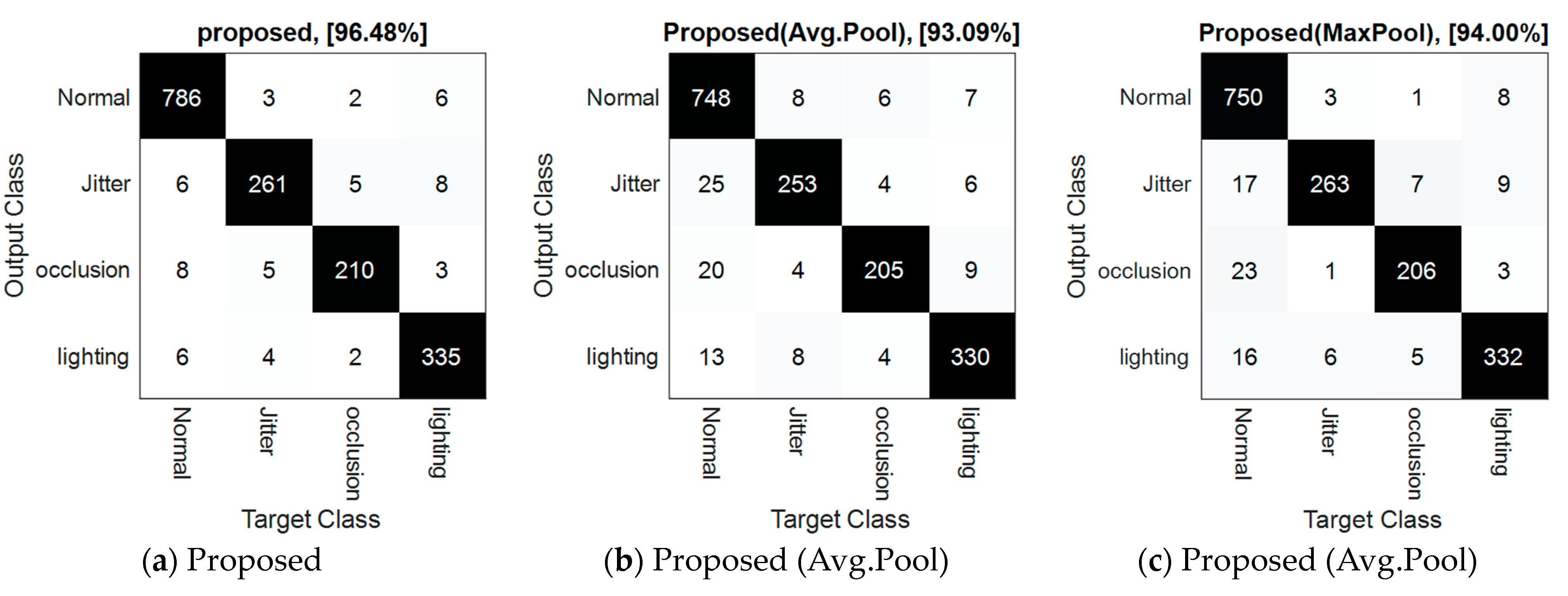
3.2. Performance of the Proposed Method in Anomaly Detection

The proposed method was implemented using MATLAB 2021a software. All experiments were performed on a personal computer running the Windows 10 operating system on an Intel Core i7 processor with a processing frequency of 3.2 GHz, and 16 GB RAM. The implementation of the CNN model was performed based on the CUDA capability of the NVidia GeForce GTX 1080 graphics adapter.

To examine the effectiveness of the proposed 3D CNN model in detecting anomalies, its performance was compared with the following configurations:

• Proposed (Avg. Pooling): In this configuration, all pooling layers in the 3D CNN model used in the proposed method were of the average pooling type.
• Proposed (Max Pooling): In this configuration, all pooling layers in the 3D CNN model used in the proposed method were of the max pooling type.
• Two-dimensional CNN: In this configuration, the anomaly detection is performed using the 2D CNN model only. It should be noted that in this case, the learning model is fed with one frame each time.

In addition to the above three cases, the performance of the proposed 3D CNN model in anomaly detection was compared with the ResNet50 and VGG-16 networks.

In Figure 4, the average accuracy of the proposed method for identifying anomalies in videos is compared with other methods. It should be noted that the results presented in this figure and other graphs in this section are the aggregate results of 10 repetitions of the experiments. Based on Figure 4, the proposed method can achieve an accuracy of 96.48% in identifying video anomalies, and it outperforms the compared methods. On the other hand, if the hybrid pooling layers of the proposed 3D CNN are replaced with average pooling layers, the detection accuracy will decrease to 93.09%. Similarly, if the hybrid pooling strategy is ignored and feature extraction is performed by the Max Pooling-based CNN model, the detection of anomalies can be performed with an accuracy of 94%. In contrast, in the case of replacing the proposed 3D CNN with a 2D CNN (with a similar architecture), the detection accuracy decreases to 89.33%. These comparisons indicate that firstly, the use of the proposed 3D CNN model can perform better compared to 2D convolutional models such as 2D CNN, ResNet50, and VGG-16, and increase the detection accuracy by at least 5.15%; secondly, comparing the performance of the hybrid pooling mechanism with CNN models using static pooling functions demonstrates that this mechanism is capable of extracting more accurate anomaly-related features, and based on the extracted features, the detection accuracy can be increased by at least 3.39%. These results demonstrate the effectiveness of the techniques employed in the proposed method for improving the accuracy of video anomaly detection.

The confusion matrix can provide more detailed insights into the performance of classification methods in identifying various video anomalies. In Figure 5, the confusion matrix of the proposed method and other methods in classifying database samples is presented.

In these confusion matrices, each column represents the actual labels of the test samples, and the rows represent the labels assigned by each classification method. For example, in Figure 5a, out of 806 samples belonging to the “normal” class (the sum of values in the first column of the matrix), the proposed method correctly classified 786 samples, and only 20 samples were misclassified into other categories. The interpretation of classification results for other existing categories is similarly possible. The proposed 3D CNN model could correctly classify 95.6% of jitter anomalies. On the other hand, the performance of this model in correctly classifying occlusion and lighting anomalies was 95.89% and 95.17%, respectively, which are significantly higher than the compared methods. Overall, the comparison of these confusion matrices shows that the proposed method has superiority over other methods in classifying samples of most categories and managed to increase the accuracy of anomaly detection by at least 3.39%.

Figure 6 compares the performance of different methods in detecting various video anomalies based on precision, recall, and F-measure metrics in the database.

In each of the plotted graphs in Figure 6a–c, the first dimension represents the classes related to video anomalies, and the second dimension corresponds to the compared methods. By examining these graphs, it can be inferred that the proposed method, when using layers of hybrid pooling in 3D CNN, can classify different categories with higher efficiency compared to other methods. Figure 6d presents the average metrics of precision, recall, and the F-measure. These graphs demonstrate the overall performance of different methods in terms of classification quality. Furthermore, the numerical results obtained from the experiments conducted in this section are presented in

Table 2. Comparison of the performance of the models in anomaly detection.

Method	Accuracy	F-Measure	Recall	Precision
Proposed	96.4848	95.6734	96.0460	95.3241
Proposed (AvgPool)	93.0909	92.0620	93.2088	91.0522
Proposed (MaxPool)	94	93.1615	94.4428	92.0419
2D CNN	89.3333	87.909	89.1707	86.8763
ResNet50	91.3333	89.8329	90.9986	88.8237
VGG-16	90.5455	88.7227	89.7765	87.7941

.

The comparison of the accuracy, precision, recall, and F-measure metrics in Table 2 and Figure 6 confirms that the proposed method can identify various video anomalies with higher quality compared to the other models. Based on these results, the proposed method can improve the metrics of precision, recall, and the F-measure. Higher precision validates that the outputs generated by the proposed method are more likely to be correct for each type of anomaly compared to other methods. Additionally, higher recall indicates that the proposed method has been able to correctly identify a higher rate of samples belonging to different anomaly types. Figure 7 illustrates the ROC curve obtained from the detection of various anomalies in video samples.

Based on the data presented in Figure 7, the proposed method demonstrates superior true positive rates and lower false positive rates compared to the other methods being compared. Additionally, the proposed method exhibits a larger area under the ROC curve. Thus, it can be inferred that the method proposed in this paper achieves a better performance in accurately categorizing different video anomalies based on their frame sequences.

3.3. Performance of the Proposed Method in Quality Assessment

In this section, the performance of the proposed hybrid model is evaluated in video quality assessment using SROCC, PLCC, and CCC criteria. In this experiment, the performance of the proposed model has been evaluated in two modes.

-

Proposed (3D + 2D CNNs): In this case, according to the procedure presented in Section 3, quality assessment is performed based on the combination of 3D CNN and 2D CNN features.

-

Proposed (2D CNN Only): In this case, only the 2D CNN model is used to assessment of video quality. In other words, the features extracted by 3D CNN are ignored in the proposed model. The purpose of comparing the proposed method with this state is to evaluate the effectiveness of the proposed hybrid strategy.

In addition to the above situations, the performance of the proposed method was compared with the RANKIQA [21], DB-CNN [22], and LIQA [23] methods. Figure 8 shows the results of quality assessment on two samples of the database.

As shown in Figure 8, in similar scenes, the quality of the left image is significantly higher than that of the right image. The score of the left image is 60.1215 and the score of the right image is 40.2418. The proposed hybrid model can objectively evaluate image quality in real scenes. The better image quality is, the higher the evaluation score is, and it is more consistent with subjective evaluation.

Figure 9 compares the performance of different methods in quality assessment using SROCC, PLCC, and CCC criteria. In this figure, the first dimension represents each of the SROCC, PLCC, and CCC metrics, while the second dimension represents quality assessment methods.

The results presented in Figure 9 show that the proposed method is superior to the compared methods in terms of the evaluated metrics. According to the obtained results, if only the 2D CNN model is used to assess the quality of samples, correlation-based criteria will be significantly reduced. This feature shows that the 3D CNN model can be effective in describing the temporal features of video frames for quality assessment purposes, so combining the features of these two CNN models can be effective in obtaining a more accurate model for quality assessment. According to these results, the LIQA [23] model has the closest performance to the proposed approach, but the simplicity of the proposed architecture compared to methods such as LIQA or DB-CNN makes our method suitable for real-world applications.

Figure 10 compares the performance of different methods using a Taylor diagram. In this diagram, the efficiency of methods in quality assessment was evaluated in terms of correlation, standard deviation, and normalized RMSD at the same time.

Figure 10 shows that the quality values assessed by the proposed method, in addition to being consistent with the subjective quality values, also have fewer differences. These results show that the scale of quality values produced by the proposed method is more consistent with the subjective quality values and this indicates the ability to understand and analyze the output of the proposed model better than other methods.

Table 3. The performance of different methods in terms of quality assessment.

Method	PLCC	SRCC	CCC
Proposed (3D + 2D CNNs)	0.9014	0.8926	0.8972
Proposed (2D CNN Only)	0.7931	0.7729	0.7764
RANKIQA [21]	0.8276	0.8175	0.8196
DB-CNN [22]	0.8661	0.8569	0.8617
LIQA [23]	0.8891	0.8806	0.8854

summarizes the performance of different methods in terms of quality assessment.

3.4. Conclusions

In this paper, a new model for quality assessment and anomaly detection in airport surveillance systems was presented. The proposed model utilizes a 3D CNN and a 2D CNN for achieving fulfilling these tasks. The 3D CNN in the proposed model can be used individually for anomaly detection in input videos. The results show that the proposed 3D CNN model was able to correctly detect anomalies in surveillance videos with an average accuracy of 96.48%, which is at least 3.39% higher than the compared methods. On the other hand, the 3D CNN and the 2D CNN cooperated to extract the quality-related features from the input. In this case, the concatenated features of these two CNNs were used by a regression layer to predict the quality of the input video. The results showed that the quality values assessed by the proposed method, in addition to being consistent with the subjective quality values, also had fewer differences. The higher accuracy and lesser complexity of the model prove the efficiency of this approach for being used in real-world scenarios.

References

1. Lyu, Z.; Luo, J. A surveillance video real-time object detection system based on edge-cloud cooperation in airport apron. Appl. Sci. 2022, 12, 10128. [Google Scholar] [CrossRef]
2. Balasundaram, A.; Dilip, G.; Manickam, M.; Sivaraman, A.K.; Gurunathan, K.; Dhanalakshmi, R.; Ashokkumar, S. Abnormality identification in video surveillance system using DCT. Intell. Autom. Soft Comput. 2021, 32, 693–704. [Google Scholar] [CrossRef]
3. Thai, P.; Alam, S.; Lilith, N.; Nguyen, B.T. A computer vision framework using convolutional neural networks for airport-airside surveillance. Transp. Res. Part C Emerg. Technol. 2022, 137, 103590. [Google Scholar] [CrossRef]
4. Zhang, X.; Shu, C.; Li, S.; Wu, C.; Liu, Z. AGVS: A New Change Detection Dataset for Airport Ground Video Surveillance. IEEE Trans. Intell. Transp. Syst. 2022, 23, 20588–20600. [Google Scholar] [CrossRef]
5. Zhang, X.; Qiao, Y. A video surveillance network for airport ground moving targets. In Proceedings of the Mobile Networks and Management: 10th EAI International Conference, MONAMI 2020, Chiba, Japan, 10–12 November 2020; Proceedings 10. Springer International Publishing: Berlin/Heidelberg, Germany, 2020; pp. 229–237. [Google Scholar]
6. Chen, P.; Li, L.; Wu, J.; Dong, W.; Shi, G. Contrastive self-supervised pre-training for video quality assessment. IEEE Trans. Image Process. 2021, 31, 458–471. [Google Scholar] [CrossRef]
7. Dost, S.; Saud, F.; Shabbir, M.; Khan, M.G.; Shahid, M.; Lovstrom, B. Reduced reference image and video quality assessments: Review of methods. EURASIP J. Image Video Process. 2022, 2022, 1–31. [Google Scholar] [CrossRef]
8. Kumar, C.; Singh, S. Security standards for real time video surveillance and moving object tracking challenges, limitations, and future: A case study. Multimedia Tools Appl. 2023, 1–32. [Google Scholar] [CrossRef]
9. Pareek, P.; Thakkar, A. A survey on video-based human action recognition: Recent updates, datasets, challenges, and applications. Artif. Intell. Rev. 2021, 54, 2259–2322. [Google Scholar] [CrossRef]
10. Streijl, R.C.; Winkler, S.; Hands, D.S. Mean opinion score (MOS) revisited: Methods and applications, limitations and alternatives. Multimedia Syst. 2016, 22, 213–227. [Google Scholar] [CrossRef]
11. Barman, N.; Zadtootaghaj, S.; Schmidt, S.; Martini, M.G.; Möller, S. An objective and subjective quality assessment study of passive gaming video streaming. Int. J. Netw. Manag. 2020, 30, e2054. [Google Scholar] [CrossRef]
12. Sara, U.; Akter, M.; Uddin, M.S. Image quality assessment through FSIM, SSIM, MSE and PSNR—A comparative study. J. Comput. Commun. 2019, 7, 8–18. [Google Scholar] [CrossRef]
13. Wang, Z.; Li, Q. Information content weighting for perceptual image quality assessment. IEEE Trans. Image Process. 2010, 20, 1185–1198. [Google Scholar] [CrossRef] [PubMed]
14. Maalouf, A.; Larabi, M.C. CYCLOP: A stereo color image quality assessment metric. In Proceedings of the 2011 IEEE International Conference on Acoustics, Speech and Signal Processing (ICASSP), Prague, Czech Republic, 22–27 May 2011; pp. 1161–1164. [Google Scholar]
15. Omari, M.; Abdelouahed, A.A.; Hassouni, M.E.; Cherif, H. Improving Reduced Reference Image Quality Assessment Methods By Using Color Information. Int. J. Comput. Inf. Syst. Ind. Manag. Appl. (IJCISIM) 2018, 10, 183–196. [Google Scholar]
16. Gupta, P.; Moorthy, A.K.; Soundararajan, R.; Bovik, A.C. Generalized Gaussian scale mixtures: A model for wavelet coefficients of natural images. Signal Process. Image Commun. 2018, 66, 87–94. [Google Scholar] [CrossRef]
17. Mittal, A.; Moorthy, A.K.; Bovik, A.C. No-reference image quality assessment in the spatial domain. IEEE Trans. Image Process. 2012, 21, 4695–4708. [Google Scholar] [CrossRef] [PubMed]
18. Yan, Q.; Gong, D.; Zhang, Y. Two-stream convolutional networks for blind image quality assessment. IEEE Trans. Image Process. 2018, 28, 2200–2211. [Google Scholar] [CrossRef] [PubMed]
19. Kang, L.; Ye, P.; Li, Y.; Doermann, D. Convolutional neural networks for no-reference image quality assessment. In Proceedings of the IEEE Conference on Computer Vision and Pattern Recognition, Honolulu, HI, USA, 21–26 July 2014; pp. 1733–1740. [Google Scholar]
20. Gu, K.; Zhai, G.; Yang, X.; Zhang, W. Deep learning network for blind image quality assessment. In Proceedings of the 2014 IEEE International Conference on Image Processing (ICIP), Paris, France, 27–30 October 2014; IEEE: New York City, NY, USA; pp. 511–515. [Google Scholar]
21. Liu, X.; Van De Weijer, J.; Bagdanov, A.D. Rankiqa: Learning from rankings for no-reference image quality assessment. In Proceedings of the IEEE International Conference on Computer Vision, Macao, China, 4–8 December 2017; pp. 1040–1049. [Google Scholar]
22. Zhang, W.; Ma, K.; Yan, J.; Deng, D.; Wang, Z. Blind image quality assessment using a deep bilinear convolutional neural network. IEEE Trans. Circuits Syst. Video Technol. 2020, 30, 36–47. [Google Scholar] [CrossRef]
23. Liu, J.; Zhou, W.; Li, X.; Xu, J.; Chen, Z. LIQA: Lifelong blind image quality assessment. IEEE Trans. Multimedia 2022, 25, 5358–5373. [Google Scholar] [CrossRef]
24. Lim, A.; Ramesh, B.; Yang, Y.; Xiang, C.; Gao, Z.; Lin, F. Real-time optical flow-based video stabilization for unmanned aerial vehicles. J. Real-Time Image Process. 2019, 16, 1975–1985. [Google Scholar] [CrossRef]
25. Zhang, W.; Shi, X.; Jin, T.; Chen, S.; Xu, Y.; Sun, W.; Xue, Y.; Yu, Z. A moving object detection algorithm of jitter video. In Proceedings of the 2019 4th Asia-Pacific Conference on Intelligent Robot Systems (ACIRS), Nagoya, Japan, 13–15 July 2019; IEEE: New York City, NY, USA; pp. 63–67. [Google Scholar]
26. Lejmi, W.; Khalifa, A.B.; Mahjoub, M.A. Challenges and methods of violence detection in surveillance video: A survey. In Proceedings of the Computer Analysis of Images and Patterns: 18th International Conference, CAIP 2019, Salerno, Italy, 3–5 September 2019; Proceedings, Part II 18. Springer International Publishing: Berlin/Heidelberg, Germany, 2019; pp. 62–73. [Google Scholar]
27. Zhu, H.; Wei, H.; Li, B.; Yuan, X.; Kehtarnavaz, N. A review of video object detection: Datasets, metrics and methods. Appl. Sci. 2020, 10, 7834. [Google Scholar] [CrossRef]
28. Ning, C.; Menglu, L.; Hao, Y.; Xueping, S.; Yunhong, L. Survey of pedestrian detection with occlusion. Complex Intell. Syst. 2021, 7, 577–587. [Google Scholar] [CrossRef]
29. Li, F.; Li, X.; Liu, Q.; Li, Z. Occlusion handling and multi-scale pedestrian detection based on deep learning: A review. IEEE Access 2022, 10, 19937–19957. [Google Scholar] [CrossRef]
30. Ansari, M.A.; Singh, D.K. Human detection techniques for real time surveillance: A comprehensive survey. Multimedia Tools Appl. 2021, 80, 8759–8808. [Google Scholar] [CrossRef]
31. Wu, C.; Shao, S.; Tunc, C.; Satam, P.; Hariri, S. An explainable and efficient deep learning framework for video anomaly detection. Clust. Comput. 2021, 25, 2715–2737. [Google Scholar] [CrossRef] [PubMed]
32. Sultani, W.; Chen, C.; Shah, M. Real-world anomaly detection in surveillance videos. In Proceedings of the IEEE Conference on Computer Vision and Pattern Recognition, Salt Lake City, UT, USA, 18–23 June 2018; pp. 6479–6488. [Google Scholar]
33. Crnjanski, J.; Krstić, M.; Totovic, A.R.; Pleros, N.; Gvozdić, D. Adaptive sigmoid-like and PReLU activation functions for all-optical perceptron. Opt. Lett. 2021, 46, 2003–2006. [Google Scholar] [CrossRef]
34. Tong, Z.; Tanaka, G. Hybrid pooling for enhancement of generalization ability in deep convolutional neural networks. Neurocomputing 2019, 333, 76–85. [Google Scholar] [CrossRef]
Figure 1. The structure of the proposed method for anomaly detection and quality assessment.
Electronics 13 00749 g001
Figure 2. The proposed 3D CNN model for anomaly detection.
Electronics 13 00749 g002
Figure 3. The structure of the proposed 2D CNN for quality assessment.
Electronics 13 00749 g003
Figure 4. Average accuracy of the proposed method and other methods in anomaly detection.
Electronics 13 00749 g004
Figure 5. Confusion matrix of different methods of video anomaly detection.
Electronics 13 00749 g005aElectronics 13 00749 g005b
Figure 6. Comparison of the performance of different methods based on (a) precision, (b) recall, and (c) F-measure for each class, and (d) average of these metrics.
Electronics 13 00749 g006
Figure 7. ROC curve resulting from the detection of video anomalies by various models.
Electronics 13 00749 g007
Figure 8. Quality assessment by the proposed method on two samples of the database.
Electronics 13 00749 g008
Figure 9. Comparing the performance of different methods in quality assessment using SROCC, PLCC, and CCC criteria.
Electronics 13 00749 g009
Figure 10. Comparing the performance of different methods in quality assessment using SROCC, PLCC, and CCC.
Electronics 13 00749 g010