Article

Multi-Indicator Fused Resilience Assessment of Power Grids Considering Wind-Photovoltaic Output Uncertainty during Typhoon Disasters

1
National Key Laboratory of Power Systems in Shenzhen, Shenzhen International Graduate School, Tsinghua University, Shenzhen 518055, China
2
Shenzhen National Climate Observatory, Shenzhen 518040, China
*
Author to whom correspondence should be addressed.
Electronics 2024, 13(4), 745; https://doi.org/10.3390/electronics13040745
Submission received: 31 December 2023 / Revised: 26 January 2024 / Accepted: 30 January 2024 / Published: 13 February 2024
(This article belongs to the Special Issue Advances in Enhancing Energy and Power System Stability and Control)

Abstract

:
Extreme weather events such as typhoons pose a serious threat to the safe operation of power grids. In the field of power system resilience assessment during typhoon disasters, a parametric typhoon wind field model combined with actual historical meteorological data has not been well adopted, and the conventional renewable energy uncertainty modeling methods are not suitable for typhoon disaster periods. In this paper, a multi-indicator fused resilience assessment strategy considering wind-photovoltaic uncertainty and component failure during typhoon disasters is proposed. Firstly, based on the actual historical meteorological data of typhoons, an uncertainty model of typhoon wind speed is established by a rolling non-parametric Dirichlet process Gaussian mixture model. Then, a spatial–temporal contingency set is constructed by considering the best-fit wind field model and stress–strength interference model for failure probability of transmission lines. On this basis, a holistic resilience assessment framework is established from the perspectives of priority, robustness, rapidity, and sustainability, and the entropy weight method combined with the technology for order preference by similarity to an ideal solution is leveraged to obtain the comprehensive resilience indicator. Finally, numerical studies are performed on the IEEE-30 bus test system to identify vulnerable lines and improve system resilience during typhoon disasters.

1. Introduction

In recent years, the frequent occurrence of extreme natural disasters has posed serious challenges to the power grid. Although the power grid has taken a series of security and stability measures to ensure its safe and stable operation, in some extreme events (such as extreme weather), the last line of defense of the power grid is likely to be breached, resulting in large-scale blackouts. In 2012, Hurricane Sandy hit the East Coast of the United States, causing power outages for over 7.5 million users in 15 states and Washington, D.C. [1]. In 2018, Typhoon Mangkhut caused a power outage on 416 10 kV transmission lines of the Shenzhen power grid and a momentary loss of voltage in 6 110 kV substations, affecting 182,400 users. Super Typhoon Lekima, which landed on the southeast coast of China in August 2019, caused more than 4000 line faults and a power outage of 6,769,500 users. To a certain extent, this shows that the power grid is insufficient to cope with such high-impact low-probability (HILP) events [2]. Owing to the characteristics of HILP, once the extreme event occurs, it will cause huge losses, and proactive measures must be taken to cope with the high impact of the extreme events. In this context, the concept of power grid resilience has been put forward by the academic community, industry, and government departments to describe the ability of the power grid to prevent, resist, respond, and quickly restore power supply in the face of extreme events [3], among which extreme natural disasters (such as typhoons, rainstorms, and ice hazards) are a typical representative of such extreme events. With the increasing proportion of renewable energy generation in the power grid, photovoltaic (PV) power output is closely related to incident irradiance and temperature, while wind power output is closely related to wind speed and air density [4]. It is noteworthy that the risks posed by climate change and the integration of renewable energy are not independent but interrelated [5]. Obviously, renewable-energy-based power grids will be more susceptible to extreme weather conditions, thus posing a serious threat to the safety and stability of the power grid [6]. Therefore, it is of great practical significance to explore the resilience of power grids against extreme natural disasters such as typhoons.
Scholars have made significant research contributions in assessing power grid resilience under extreme typhoon weather [7]. In terms of modeling typhoon weather conditions [8], although parametric typhoon wind field models have been widely studied in the fields of meteorology and building structural reliability [9], their application in power system resilience is still relatively rare. Most of the existing literature only utilizes a certain wind field model and hypothetical data, without verifying the applicability of the model or comparing which of these models is better. Several studies have employed physical or empirical typhoon wind field models, like Batts [10,11] and Yan Meng [12], to simulate typhoon weather conditions and determine wind speeds in the areas affected by typhoons. However, these research methods lack practical basis, and the wind speed results obtained may not match the actual situation. As the continuous refinement of typhoon track prediction algorithms progresses, it is imperative to incorporate typhoon track data to enhance the accuracy of power system resilience assessment [13]. Regarding the impact mechanism of extreme weather on the power grid, component failure probability models are commonly utilized to depict the extent of damage to the power grid under different weather conditions. Numerous studies have been conducted, utilizing an exponential function known as fragility curve based on the design wind speed of towers and lines [10,14,15], to fit the relationship between component failure probability and typhoon wind speed, thus establishing a vulnerability model for transmission lines to reflect the real-time impact of severe weather condition on the operational status of components [16]. For example, in [17], the authors utilized fragility curves to simulate the damage caused by wind to transmission lines, towers, and substations. However, this model is too idealistic to reflect the variation in wind loads imposed on the transmission lines considering the wind direction and the variation coefficient of the design wind loads. Most of the current studies consider the time-varying characteristics of extreme disasters, yet often tend to treat the system spatially as a small area in geographical extent, thereby uniformly calculating the component failure probability, ignoring the fact that extreme typhoon disasters possess the characteristics in both spatial and temporal dimensions.
The existing modeling of renewable energy output uncertainty is usually based on commonly used probability distributions (such as Weibull distribution) or relies on long-term measurement data. However, the renewable energy output under normal meteorological conditions cannot be directly applied during typhoon disasters. The analysis of power grid resilience under hurricane wind conditions from 2017 to 2050 indicates that as the penetration level of renewable energy increases, the restoration cost and capacity loss will increase dramatically [17]. A stochastic modeling approach for solar irradiance under hurricanes was developed by fusing datasets of historical global horizontal irradiance and Atlantic hurricane activity, suggesting that the environmental conditions imposed by hurricanes can substantially reduce solar power generation [18]. Reference [19] conducted a long-term reliability assessment of the Texas interconnection using multiple climate models. However, the studies considering the fluctuations in renewable energy output caused by extreme climate conditions are rarely applied to the power system resilience assessment [20], and few studies have considered the spatial–temporal uncertainty of renewable energy sources. In addition, with the development of digital technology and the widespread application of big data, the weather forecasting, information acquisition, and analysis will be updated and upgraded, and research on the data-driven method integrating meteorological data and power grid information will be more extensive [21].
In the research of resilience assessment methods and indicators, some indicators describing the power grid usually include economic indicators [22], reliability indicators [23], and system stability indicators [24]. The typical performance transitions of a power grid facing disturbance events were often divided into the pre-disaster prevention stage, the mid-disaster resistance stage, and the post-disaster recovery stage [25,26]. The research on the quantitative resilience assessment commonly employed simulation methods to simulate the dynamic performance of the power grid during fault and recovery stages by constructing optimization models [27,28]. Then, the multi-stage resilience indicators were calculated based on the optimization model results [29,30]. However, most of the current research mainly focused on evaluating specific disaster scenarios, ignoring the diversity of disasters [31] and the uncertainty of renewable energy in the power grid, and less considered multiple contingencies beyond N-3 [18,32]. In addition, the size of the missing area in the system performance curve was often used as a resilience indicator and subsequently improved [25,29,33,34]. Other resilience indicators were constructed based on graph theory [35] and statistical methods [36]. Regarding the existing studies on the resilience assessment, most of them put forward or employ a single resilience indicator to assess resilience of power grids in the face of natural disasters, which has certain limitations [37]. For instance, using the resilience trapezoidal area as a single resilience indicator makes it difficult to distinguish the impact of load loss time and degree, resulting in the same results on resilience indicators for short-term but large-loss scenarios and long-term but small-loss scenarios [38]. On the other hand, few studies employ the multidimensional resilience assessment framework [39], and the associated indicators often lack intuitiveness.
In this paper, the power grid resilience assessment method considering renewable energy output uncertainty in the face of extreme typhoon weather is elaborately investigated, and a holistic power grid resilience assessment framework is proposed. Firstly, a spatial–temporal model of typhoon events is established based on actual historical meteorological data and the typhoon wind field model to simulate the scenarios of renewable energy output and the spatial–temporal wind loads imposed on the transmission lines and towers, which realistically reflect the spatial–temporal impacts of the extreme typhoon weather from the power source and the network sides on the power grid. In particular, based on actual historical meteorological data, the temporal wind-PV output uncertainty during the typhoon event is modeled by using a rolling Dirichlet process Gaussian mixture model (DPGMM). Then, the wind loads on transmission lines and towers are calculated, and the spatial–temporal failure probabilities of the transmission lines and towers are calculated based on the stress–strength interference model. On this basis, the contingency set is screened, and the system performance curve is obtained through the optimal load shedding strategy. At the same time, combined with the system performance curve, a comprehensive assessment framework of power grid resilience is proposed, which integrates multi-dimensional resilience indicators. The entropy weight method (EWM) and the technique for order preference by similarity to an ideal solution (TOPSIS) are employed for the solution of the proposed framework. Finally, the detailed case studies are performed on an improved IEEE-30 bus test system during typhoons with different intensities, aiming to verify the effectiveness of the proposed resilience assessment framework.
The main contributions of this paper are summarized as follows:
(1)
A holistic power grid resilience assessment framework considering renewable energy output uncertainty in the face of extreme typhoon weather is proposed, aiming to effectively analyze the ability of the power grid to withstand natural disasters.
(2)
A spatial–temporal uncertainty model of typhoon wind speed is established by utilizing a rolling non-parametric DPGMM based on the actual historical meteorological data of typhoons.
(3)
The optimal wind field model and the actual typhoon best track data are leveraged to model the typhoon wind field, thereby obtaining the spatial–temporal contingency set of the power grid.
(4)
A comprehensive assessment framework of power grid resilience is constructed by employing the EWM and TOPSIS.
The remainder of the paper is organized as follows. Section 2 describes the holistic research framework and the problem formulation, including wind field model, wind-PV output uncertainty model, component failure probability model, contingency set generation strategy considering time series, optimal load shedding strategy, and comprehensive resilience assessment framework. Section 3 discusses the corresponding solution strategy for the proposed resilience framework. The detailed simulations performed on an improved IEEE-30 bus test system can be found in Section 4. Finally, a concluding remark is given in Section 5.

2. Problem Formulation

This paper presents a resilience assessment framework considering the renewable energy output uncertainty and line failure in the face of extreme typhoon weather. Based on the actual historical meteorological data and a kind of data-driven technology called rolling DPGMM, the joint probability density of wind-PV output is first modeled. Then, the applicability of the parametric typhoon wind field model is verified, and the optimal typhoon wind field models are selected to simulate the wind speeds in the geographical area of the power grid and to calculate the wind loads on the lines and towers. Based on the stress–strength interference model, the failure probability of each transmission line at different times is calculated, and the spatial–temporal contingency set is generated by applying the quasi-Monte Carlo method. On this basis, the optimal load shedding strategy is used to simulate different wind-PV output scenarios multiple times, aiming to obtain the system performance curves. Finally, a multi-indicator fused assessment framework for power grid resilience is proposed, and the EWM and TOPSIS are leveraged to determine the comprehensive resilience indicator. The corresponding holistic research framework is shown in Figure 1.

2.1. Wind Field Model

The typhoon wind field model, designed for disaster risk assessment, is capable of numerically simulating and establishing the relationship between wind speed and atmospheric pressure in areas affected by typhoons and the typhoon center. Generally, a parametric wind field model can calculate the gradient wind field by utilizing a specific wind profile function, which requires the input of key parameters including central pressure, maximum wind radius, radial wind profile shape coefficient, and moving speed and moving direction of typhoon center [40]. On this basis, taking into account the underlying surface, the boundary layer model is utilized to calculate the reduction coefficient from the gradient wind speed to the wind speed at 10 m above the surface, so that the near-surface wind field model can be obtained. The typhoon track data used in this paper come from the typhoon best track data released by Typhoon Online of the National Meteorological Center (http://typhoon.nmc.cn accessed on 15 August 2023), which serve as the input parameters for the wind field model, allowing it to output the wind speed data for any location within the affected area.

2.1.1. Key Parameter Estimation

Most typhoon wind field models necessitate the radius of maximum wind (RMW) as a key parameter. Due to the lack of relevant RMW data provided in the measured data, this study adopts a parameterized approach as shown in Equation (1) to estimate the RMW [41].
R max = e ( 5.0237 0.0247 Δ P )
where R max is the RWM, and Δ P is the pressure difference between the typhoon central pressure and peripheral pressure.

2.1.2. Gradient Layer Typhoon Model

In the typhoon wind field model, most of the initially proposed wind field models are characterized by circular symmetric wind fields [42] (such as the Rankine and Batts wind field models). To reflect the asymmetry of the wind field, the wind speed at a certain location is often regarded as the vector sum of the circulation wind speed and the moving wind speed, as shown in Equation (2). The circulation wind speed is obtained by a circular symmetric wind field model by assuming that the pressure gradient, Coriolis force, and centrifugal force are balanced, while the moving wind speed is obtained by a moving wind field model [43]. Commonly used wind field models mainly include the Rankine and Batts circular symmetric models based on Rankine vortices, the Schloemer model based on e-exponential wind fields, the Jelenianski-II model based on exponential wind fields, and the Holland [44] model proposed by using gradient wind relationships. This paper mainly focuses on the four aforementioned wind field models and conducts applicability verification using the measured typhoon data to identify and select the optimal wind field models among them.
V = V r + V m
  • Batts wind field model [45]
The Batts wind field model is a representative of the circularly symmetric wind field model, which is widely used due to its simple form, as shown in Equation (3).
V r = V max × r R max r R max V r = V max × ( R max r ) a r > R max
where Rmax is the distance between the typhoon center and the strongest wind zone, that is, the RMW; Vmax is the maximum wind speed; r is the distance from the component location to the typhoon center; and a is a constant in the range of 0.5 to 0.7 and taken as 0.5 in this paper.
2.
Schloemer wind field model [46]
The Schloemer wind field model is asymmetric, including a circular symmetric wind field and moving wind field. The circular symmetric wind field model is shown as Equation (4).
V r = V max ( R max r ) e ( 1 R max r )
The moving wind field model is shown as Equation (5).
V m = V T 3 R 3 / 2 r 3 / 2 R 3 + r 3 + R 3 / 2 r 3 / 2
where V T is the typhoon center moving speed, which can be approximately calculated by V T = β Δ L a t 2 + Δ L o n 2 Δ t if the data is missing; β is the conversion factor from latitude and longitude to kilometers, which is approximately 110.7 km/deg.
3.
Jelenianski-II wind field model [47]
The typhoon pressure model [48] is given as:
P = P c + 1 4 ( r R max ) 3 ( P P c ) 0 < r R max P = P c + ( 1 3 r 4 R max ) ( P P c ) r > R max
where P c , P are the typhoon central pressure and the peripheral pressure, respectively; P c is obtained from the typhoon best track data; P in the northwest Pacific is generally taken as 1010 hpa.
The circular symmetric wind field model is given as:
V r = V max 2 R max r R max 2 + r 2
The moving wind field model is given as:
V m = V T r r + R max 0 < r R max V m = V T R max r + R max r > R max
4.
Holland wind field model [49]
The typhoon pressure model is given as:
P = P c + ( P P c ) e ( r R max ) B B = 1.0036 + 0.0173 V max 0.0313 I n R max
The circular symmetric wind field model is given as:
V r = f 2 r 2 4 + r ρ P ( r ) r f r 2
where f = 2 sin ( l a t ) ω is Coriolis parameter; l a t is latitude of the typhoon center; ω is rotational angular velocity of the earth with a value of 7.292 × 10 5 rad / s ; ρ is the air density, usually taken as 1.29   kg / m 3 .
The moving wind speed is modeled using the following Miyazaki model [50]:
V m = V T e π r R G
where R G is the radius of the area affected by the typhoon.
Given that there is an inflow angle of approximately 20° [51] between the wind speed and the pressure gradient in the circular wind speed, the circular wind speed in both the x and y directions can be expressed as:
V r = V r ( A i + B j ) A = ( y cos θ + x sin θ ) / r B = ( x cos θ y sin θ ) / r r = ( x 2 + y 2 )
where θ is the inflow angle taken as 20°; x is the latitudinal distance from the component location to the typhoon center; y is the longitudinal distance from the component location to the typhoon center. The gradient layer wind speed is obtained by vectorially superimposing the circular and the moving wind speeds.

2.1.3. Boundary Layer Model [52]

Typhoons that can cause disasters are usually referred to near surface winds. The wind speed obtained in the gradient wind field model is the vertical average wind speed at the top of the boundary layer, and the height of the boundary layer is usually 1000 m. Therefore, the gradient average wind speed needs to be converted into near-surface wind speed using Equation (13).
α = V 10 V
where V 10 is the wind speed at a height of 10 m, and V is the gradient average wind speed. The value of α ranges from approximately 0.65 to 0.95 and is taken as 0.71 for cases when V is less than 40 m/s and adjusted to 0.8 when V exceeds 40 m/s.
The wind speed obtained by the above typhoon wind field model is approximately equivalent to the 1 h average wind speed, while the wind speed at the meteorological station is usually the 10 min average wind speed. Therefore, the results need to be converted. Here, the gust coefficient is defined as:
G τ , T 0 = V τ , T 0 V
where G τ , T 0 is the conversion factor between the T 0 average wind speed and the τ average wind speed, V τ , T 0 is the τ average maximum wind speed in time T 0 , and V is the T 0 average wind speed. As recommended by the World Meteorological Organization (WMO), G 600 , 3600 is taken as 1.08 for inland areas [53].

2.2. Wind-PV Output Uncertainty Model

As is widely recognized, the power output of renewable energy sources such as wind farms and PV power stations is characterized by a high degree of uncertainty. The conventional modeling of renewable energy output uncertainty is usually based on long-term renewable energy output levels or probability density fitted from long-term wind speed and solar irradiance. Given that the movement of the typhoon center and the increase or decrease in typhoon intensity will have both temporal and spatial impacts on renewable energy output, it is crucial to consider the temporal and spatial correlations of renewable energy output when modeling during extreme typhoon events. This paper will leverage the rolling non-parametric DPGMM [54] method to model the uncertainties of wind farm output and PV station output, and employ the measured data to sequentially fit and sample the renewable energy output scenarios at the current calculated time. The wind speed and PV station output data within one hour before and after each time are used as input data for the rolling DPGMM [55] to model the probability density of wind-PV output uncertainty at the current time, as shown in Equation (15). When K t is a positive integer greater than one, Equation (15) is a generalized expression for a Gaussian mixture model (GMM), whereas in DPGMM, K t is an output parameter, which is the number of the mixtures of Gaussian distribution that the model automatically infers based on the input data.
P t ( x | β t , Ω t ) = k = 1 K t β t k N ( x μ t k , Σ t k ) t { 1 , 2 , 3 T } k = 1 K β t k = 1
where x = [ x 1 , x 2 , , x D ] is D-dimensional random variables; β t k is the weight coefficient of the kth mixed Gaussian distribution at time t ; β t = { β t k } k = 1 K t is vector of weighting coefficients; μ t k , Σ t k are the mean vector and covariance matrix of the kth mixed Gaussian distribution; Ω t = { μ t k , Σ t k } k = 1 K t is parameter space; K t is Gaussian components inferred by the model itself. DPGMM is a non-parametric Bayesian model, and the parameters β t , Ω t , and K t of the model can be solved by the variational Bayesian inference (VBI) method. After solving the parameters, the probability density functions of wind speed and PV output at each time are obtained, and the probability density are sampled to obtain several scenarios that conform to the probability densities of the wind speed and PV output. Then, the wind farm output during the typhoon event is calculated through Equation (16) to obtain wind-PV output uncertainty scenarios eventually.
P W F = 0 v v c i   o r   v > v c o n P w r v 3 v c i 3 v r 3 v c i 3 v c i < v v r n P w r v r < v v c o
where v c i , v c o , v r are the cut-in, cut-out, and rated wind speed of wind turbines; P w r is rated power of the wind turbines; n is number of wind turbines in the wind farms.

2.3. Component Failure Probability Model

The strong winds generated by typhoons impose enormous wind pressure on overhead transmission lines. Once the wind pressure exceeds the mechanical strength of the transmission lines and towers, failures such as line disconnection and tower collapse will occur. Meanwhile, structural fatigue and aging will also increase the probability of line failure. In this paper, the wind loads on the lines and towers are calculated according to the real-time wind speeds, and the real-time failure probability of the transmission lines is dynamically analyzed. In the Chinese standard “Code for design of 110 kV~750 kV Overhead Transmission Lines” [56], the formula for calculating horizontal wind load of lines is given as follows:
W x = 1 1600 α μ z μ s c β c d L p V 2 sin 2 θ
where W x is the horizontal wind load perpendicular to the wire axis in N ; α is the unevenness coefficient of wind pressure that varies with wind speed V ; μ z is the variation coefficient of wind pressure height, and it is taken as 1.38, which is the value of class A ground roughness with 10 m height above the ground; μ s c is the wire body size factor, and it is taken as 1.1 in this paper; β c is the wind load adjustment factor for 500 kV and 750 kV transmission lines acting on the tower, which is taken as one for lines with lower voltage levels in this paper; d is the outer diameter of wire, which is taken as 18 mm in this paper; L p is the tower horizontal gear distance, which is taken as 300 m; V is wind speed in meters per second at a reference height of 10 m; θ is the angle between the wind direction and the axial direction of the wire.
The formula for calculating the wind load on the towers is given as follows:
W s = 1 1600 μ z μ s β z A S V 2
where W S is tower wind load in k N ; μ z is the variation coefficient of wind pressure height, and it is taken as 1.80, which is value of class A ground roughness with 20 m height above the ground; μ s is the body shape factor, which is taken to be an approximate value of two; β z is the tower wind load adjustment factor, which increases as the tower height increases, and it is taken as the approximate value of 1.25; A s is the projected area of the structure subjected to wind pressure, which is approximated to be 20 m2.
Given the inherent randomness of wind speed over time, the wind load acting on the lines and towers is treated as a random variable. Therefore, for the period of calculation, the wind loads are assumed to follow a normal distribution with the mean value of the wind speed at the current moment. Similarly, according to the variation coefficient of component design load defined by the IEC standard [57], the standard deviation of line and tower design loads can be obtained as follows:
δ = μ Z
where μ is the mean value of the component design load; the line variation factor Z is taken as 0.03; the tower variation factor Z is taken as 0.10. When the component design wind load exceeds the actual wind load, the component can be operated reliably; conversely, when the component design wind load is less than the actual wind load, the component may fail. It is assumed that the component design wind loads and actual wind loads follow probability distributions g ( W ) and f ( w ) , respectively, and the failure probability of the lines and the towers in this period can be obtained by the stress–strength interference method [58], as shown in Equation (20) and Figure 2.
p ( w > W ) = 1 p ( w < W ) = 1 0 + f ( w ) w + g ( W ) d W d w
The lines and towers are regarded as a series system, and the normal operation of the transmission lines requires all lines and towers to operate normally. Therefore, the line failure probability can be calculated as:
p i , t ( V ) = 1 k = 1 m ( 1 p k , i , t t o w e r ( V ) ) j = 1 n ( 1 p j , i , t l i n e ( V ) )
where p i , t is failure probability of the ith transmission line at time t; m is the number of towers in the ith transmission line; n is the number of spans in the ith transmission line; p k , i , t t o w e r is the failure probability of the kth tower in the ith transmission line at time t; p j , i , t l i n e is failure probability of the wire in the jth span in the ith transmission line at time t.

2.4. Contingency Set Generation Strategy Considering Time Series

Usually, the method of sampling the failure probability of different components at each moment using Monte Carlo Simulation does not consider the fault duration and the repair time of the components. In this study, the current component failure probability and the component state at the previous stage need to be considered when sampling the current state, and it is assumed that the component repairs are completed within tr hours after the typhoon warning, and thereafter the typhoon failure probability is 0 whilst the power supply is restored. The component state at time t can be calculated by Equation (22).
p m ( t ) = 1 π ( t 1 ) ( 1 p ( t ) ) t = 1 , 2 , t e + t r 1 0 t = t e + t r , , T
where π ( t 1 ) is the component state at time t − 1, 1 refers to normal operation, 0 refers to fault state, and π ( 0 ) is 1; p ( t ) is the component failure probability calculated by Equation (21); t e is the time when the typhoon warning is canceled.

2.5. Optimal Load Shedding Strategy

During typhoon disasters, multiple contingencies often occur in the power grid, which is likely to be disaggregated into several subsystems, and at the same time, the power grid dispatchers will take measures such as generator tripping or load shedding to ensure the safety of the system. In this paper, the amount of the survived load is employed to describe the system performance in order to simulate the power grid response to the actual fault conditions, and the optimal load shedding model as shown in Equation (23) considering the importance of the loads is used to calculate the amount of load shedding on the typhoon events at different stages under different scenarios shown as follows:
min   f L C = ε P L C i s . t . P i ( V , δ ) = P g i + P w i P d i + P L C i     Q i ( V , δ ) = Q g i + Q w i Q d i + Q L C i   P g i min P g i P g i max   Q g i min Q g i Q g i max   S i j S i j max   V i min V i V i max   0 P L C i P d i   P i ( V , δ ) = V i V j ( G i j cos δ i j + B i j sin δ i j )   Q i ( V , δ ) = V i V j ( G i j sin δ i j B i j cos δ i j )
where i , j are the bus numbers; ε is the weighted parameter of load base on the importance of the users (four for the first-level load, two for the second-level load, and one for the third-level load); P i and Q i are the active and reactive powers injected to the bus i ; P L C i and Q L C i are the active and reactive powers of the shedding loads at bus i ; V i is the voltage magnitude of bus i ; P g i and Q g i are the active and reactive powers of generator at bus i ; P w i and Q w i are the active and reactive powers of renewable energy output at bus i ; P d i and Q d i are the active and reactive powers of load at bus i ; S i j is the apparent power of the line connecting to the bus i and bus j ; G i j and B i j are the conductance and susceptance between bus i and bus j ; δ i j is the voltage phase angle difference between bus i and bus j . In this study, the solution of the aforementioned load shedding model is carried out using the software MATPOWER 7.1 [59] based on the generated contingency set.

2.6. Comprehensive Resilience Assessment Framework

As mentioned above, many current studies define the resilience indicator as the integral of the difference between the pre-defined system performance indicators at time t and the performance indicator before or after recovery. However, it should be noted that using only the amount of load shedding as an indicator cannot reflect the important characteristics that can also reflect system resilience, such as duration of load shedding, maximum amount of load shedding, and other existing performance indicators. In this paper, some crucial indicators such as critical load shedding ratio, load shedding area, maximum amount of load shedding, load loss time, load recovery time, and duration of load shedding, established from the perspectives of priority, robustness, rapidity, and sustainability, as shown in Table 1 and Figure 3, will be fused to conduct the comprehensive resilience assessment for the power grid to be studied. In Table 1, R1 is the critical load shedding ratio in the range of [ ε 3 , ε 1 ] , and the smaller the value, the better the system resilience; R2 is the load shedding area in the range of [0, Pd·T], and the smaller the value, the better the system resilience; R3 is the maximum amount of load shedding in the range of [0, Pd], and the smaller the value, the better the system resilience; R4, R5, and R6 are the load loss time, the load recovery time, and the duration of load shedding, respectively, and the larger the value of R4 as well as the smaller the values of R5 and R6, the better the system resilience. Here, the EWM [60] combined with the TOPSIS [61] is employed to implement a comprehensive and objective system resilience assessment.
The basic process of objective weighting using the EWM combined with TOPSIS includes the following four steps: (i) the original indicators are standardized into the same type of indicators (generally standardized to be a maximization-type indicator, referred to forward normalization); (ii) the forward-normalized matrix is normalized; (iii) the entropy of each indicator is computed to objectively assign weights to the indicators; (iv) the distances between the evaluation values and the optimal and worst solutions are computed and normalized to obtain the final resilience results.

3. Solution Strategy

Regarding the comprehensive resilience assessment framework proposed in this paper, involving a typhoon wind field model, a spatial–temporal failure probability model, a wind-PV output uncertainty model, and a comprehensive resilience assessment method based on the optimal load shedding strategy, the corresponding solution flow chart is shown in Figure 4, and the specific steps are outlined as follows:
  • Input initial system data, geographic location data of the components, historical wind speed data of super typhoon, severe typhoon and severe tropical storm, PV output data, and the typhoon best track data.
  • Perform applicability verification using the measured typhoon data to identify and select the optimal wind field models.
  • Utilize the typhoon best track data to simulate the wind field within the affected area based on the optimal wind field model to obtain wind speeds at different locations of the components.
  • Calculate the spatial–temporal failure probability of the components and employ a quasi-Monte Carlo sampling technique to obtain the spatial–temporal contingency set.
  • Construct a spatial–temporally correlated wind-PV joint probability density function based on the rolling DPGMM, and utilize the variational Bayesian inference [54] to solve the model parameters.
  • Utilize a Monte Carlo sampling technique to sample the wind-PV joint probability density function and further obtain 10 typical scenarios based on the scenario analysis method.
  • Select the wind-PV output scenario S N as one and the contingency scenario S F as one to initiate the simulation.
  • Check whether the power grid is split and conduct islanding treatment.
  • Utilize the optimal load shedding strategy to simulate the current scenario in multiple time periods and obtain the system performance curve.
  • Simulate the next wind-PV output scenario, then go to (8) and simulate the next contingency scenario after simulating all wind-PV output scenarios. After completing all contingency scenarios, go to (11).
  • Calculate the expected amount of the survived load for all scenarios to obtain multidimensional resilience indicators, and then derive the comprehensive resilience indicator through EWM and TOPSIS methods.
  • Output the comprehensive resilience assessment results for the power grid under extreme typhoon weather conditions.

4. Case Study

The case study is carried out based on an improved IEEE-30 bus test system with the geographical wiring diagram and single-line diagram depicted in Figure 5. Two wind farms, each with an installed capacity of 10 MW, are connected to bus 21 and bus 30, respectively. Two PV power stations with installed capacity of 15 MW and 5 MW, respectively, are connected to bus 5 and bus 12. The power grid is geographically within the 112.134°~114.502° E, 21.670°~22.565° N area. The applicability verification of the parametric typhoon wind field model and system resilience assessment are performed on the test system, and then the impact of different design wind loads on the resilience assessment is analyzed.
Section 4.1 validates the applicability of the typhoon wind field model. The typhoon best track data used are released by Typhoon Online of the National Meteorological Center (http://typhoon.nmc.cn accessed on 15 August 2023), including typhoon center longitude and latitude, maximum wind speed, typhoon central pressure, and typhoon center moving speed with the time intervals of 1 h, 3 h, or 6 h of Typhoon Mangkhut, Typhoon Nida, and Typhoon Merbok. The typhoon best track data serve as the input parameters for the wind field model, allowing it to output the wind speed data for any location within the affected area. The wind speed values observed by the actual meteorological station every 1 min are compared with the simulated wind speed data obtained by the wind field model to select the optimal wind field model. At the same time, these observed wind speed values are also combined with the PV output data obtained from the actual measurement of the solar irradiation remote monitoring system [62,63] for the uncertainty modeling in Section 4.2. The PV output data used in this paper span from 1 July 2016 to 3 July 2016, with a time interval of 1 min, and are inserted into the studied typhoon impact period by 0–24 h. The period of all measured data is 6 h from the issuance of each typhoon white warning to the end of the typhoon warning.

4.1. The Applicability Verification of the Typhoon Wind Field Model

The parametric wind field models, including the Batts, Schloemer, Jelenianski, and Holland models, are implemented for Typhoon Mangkhut, Typhoon Nida, and Typhoon Merbok as described in Section 2.1. To assess the applicability of these models in simulating typhoon wind speeds, the observed wind speeds from the meteorological stations are compared with the simulation values from the wind field models. Some metrics, namely RMSE (root mean square error), MAX (maximum error), and CORR (correlation coefficient), are utilized to evaluate the performance of the different wind field models in simulating typhoon wind speeds.
From Figure 6, it can be seen that the wind speeds obtained by the wind field models exhibit similar upward and downward trends, demonstrating a strong correlation with the actual observed wind speeds. Notably, the Schloemer model yields relatively higher wind speeds, whereas the Holland model produces relatively lower wind speeds before the typhoon approaches and higher wind speeds when it approaches its extreme value. Conversely, the Jelenianski and Batts models yield wind speeds that are relatively fitting. The calculated RMSE, MAX, and CORR values are given in Table 2. Here, RMSE and MAX both reflect the difference between the simulated and observed values and are used as the main evaluation metrics of the optimal wind field model selection, while the CORR indicates the correlation between the simulated and observed values, assisting in determining whether the model is applicable or not. The CORR values given in Table 2 are all greater than 0.6, denoting a high correlation between the simulated and observed values, and the model with the minimum values of RMSE and MAX is adopted as the optimal wind field model for the typhoon event. The minimum values of RMSE and MAX for different typhoons are labeled with a background color in Table 2. The Schloemer model is found to be more suitable for simulating the wind field of Typhoon Mangkhut, while the Batts model is deemed more appropriate for simulating the wind field of Typhoon Nida and Merbok. Therefore, it becomes evident that the optimal wind field models may vary for different typhoons, contingent on natural factors such as landfall, latitude, and season.

4.2. Wind-PV Output Uncertainty Model

Given the inherent capability of DPGMM to model wind-PV output with spatial correlation, the temporal changes are effectively captured by employing rolling DPGMM across distinct time periods. Taking Typhoon Mangkhut as an example, the ten typical wind-PV output scenarios are shown in Figure 7, and a total of 80 h of wind-PV outputs from the beginning of typhoon white warning to 8 h after the end of typhoon warning are calculated. It can be seen from Figure 7 that the wind power outputs approach full power generation at or near the 35th hour, cut out at the 45th hour because the wind speed exceeds the cut-out wind speed, and subsequently resume full power generation at the 60th hour. The PV outputs vary with solar irradiance, exhibiting fluctuations throughout the day. Considering that the weather is similarly cloudy during the typhoon, the PV output is set to approximately 22% of the installed capacity.

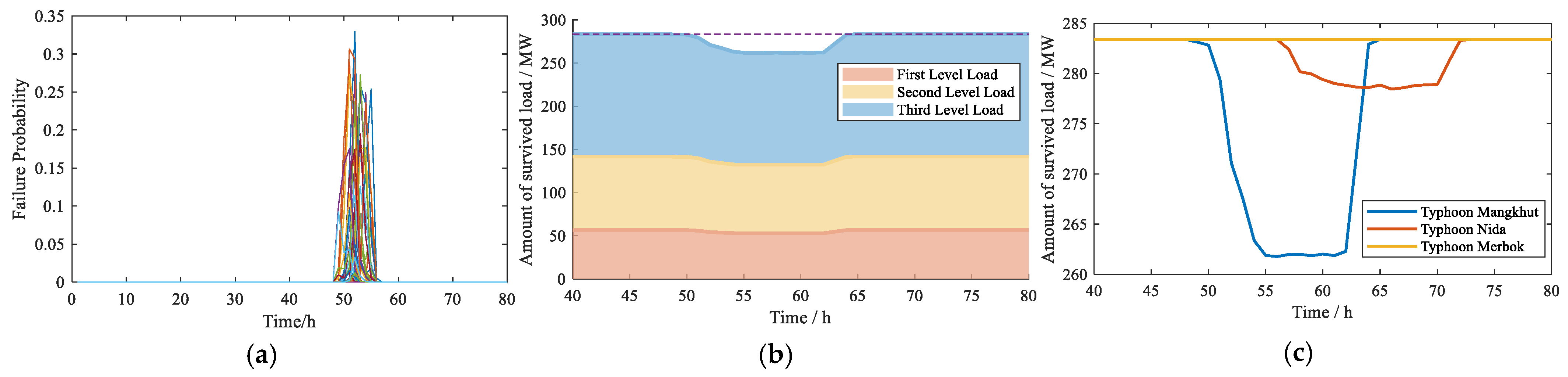
4.3. System Resilience Assessment

In this section, the Monte Carlo method is utilized to sample the spatial–temporal failure probability derived from the optimal wind field model for the contingency set. Since extreme weather events are prone to cause several line disconnections and multiple contingencies, we define the system contingencies as (N − 1)k (i.e., N − 1 − 1…−1) to represent the sequential failure characteristics of k lines if the number of lines disconnected during the typhoon impact period is k. The initial contingency sets are screened, and the scenarios from (N − 1)1 to (N − 1)k contingencies are obtained. The calculated amount of load shedding in each contingency scenario fluctuates, hence the expected amount of load shedding is determined by averaging the amount of load shedding obtained after simulations.
The wind-PV output and component failure probability are simulated during Typhoon Mangkhut, and then the comprehensive resilience assessment is conducted. From the beginning of typhoon white warning to 8 h after the end of typhoon warning, Typhoon Mangkhut affected the study area for a total of 80 h. In particular, from the 48th to the 58th hour, the wind speeds reached their peak, leading to an escalation in line failure probability and line faults. The sequential diagram illustrating line failure probability is shown in Figure 8a. The ten lines with the top 10 failure probability are shown in Table 3. It is assumed that the emergency repair team can commence repairs when the wind speed drops to 20 m/s, and the emergency repair time follows a normal distribution with a mean value of 6 h. As can be seen from Figure 8a, although the warning period of Typhoon Mangkhut is 80 h in total, the line faults emerge predominantly in the period when the wind speeds exceed 35 m/s (that is, from the 48th to the 56th hour), and the lines in adjacent geographical locations exhibit similar fault conditions.
The optimal load shedding model considering the importance of load is leveraged to prioritize the shedding of the third-level load to reserve critical load, and is more appropriate to simulate the emergency response measures of the three-level load protection. The curves of the amount of three-level survived loads are depicted in Figure 8b, in which the shedding amount of the first and the second level loads belongs to the isolated buses caused by the line faults.
The curves of the expected amount of survived load in the face of typhoons with different intensities are shown in Figure 8c. It can be seen that there is a significant amount of load shedding during Super Typhoon Mangkhut, while during Typhoon Nida, the amount of load shedding is relatively small, and Tropical Storm Merbok has little impact on the power grid. The resilience indicators from R1 to R6 under the three typhoon conditions and the multi-indicator fused comprehensive resilience indicator (CRI) are shown in Table 4, in which R4 is a maximization-type indicator, while the other indicators are minimization-type indicators. The values of indicators R1, R4, and R6 during Typhoon Mangkhut surpass those values of indicators during Typhoon Nida, but the indicators R2 and R3 are significantly worse than those values during Typhoon Nida. Consequently, during Typhoon Mangkhut, the system exhibits the lowest CRI value, which means that the system has the weakest resilience. On the other hand, during Typhoon Merbok, the system shows the highest resilience. The system performance during Typhoon Merbok closely approximates the ideal condition, yielding a CRI value of one. The CRI value of the system during Typhoon Nida is between the other two typhoon conditions. In summary, the fused CRI to some extent reveals the actual situation of the system, with larger values indicating better system resilience and smaller values indicating poorer system resilience.
The occurrence of multiple lines in the same area being affected by extreme wind speeds readily leads to (N − 1)k contingencies. A total of 1000 contingency scenarios generated from (N − 1)1 to (N − 1)9 were selected to conduct simulations, and the curves of the amount of survived load for each (N − 1)k contingency are shown in Figure 9a. The load loss increases due to the increase in k. In the event of the (N − 1)9 faults, the system experiences a loss of nearly 10% of its load. We individually screened 1000 scenarios of each contingency level and calculated the time required to simulate each contingency 1000 times. Figure 9b indicates the average time required for one simulation. It can be noticed that as the number of disconnected lines k increases, the complexity of the faults increases, and the simulation time also increases. However, the calculation time does not significantly increase with the increase in k, and it only takes about 3 s to complete one simulation for the case of (N − 1)9. Therefore, the proposed method has a good trade-off between the calculation time and accuracy.

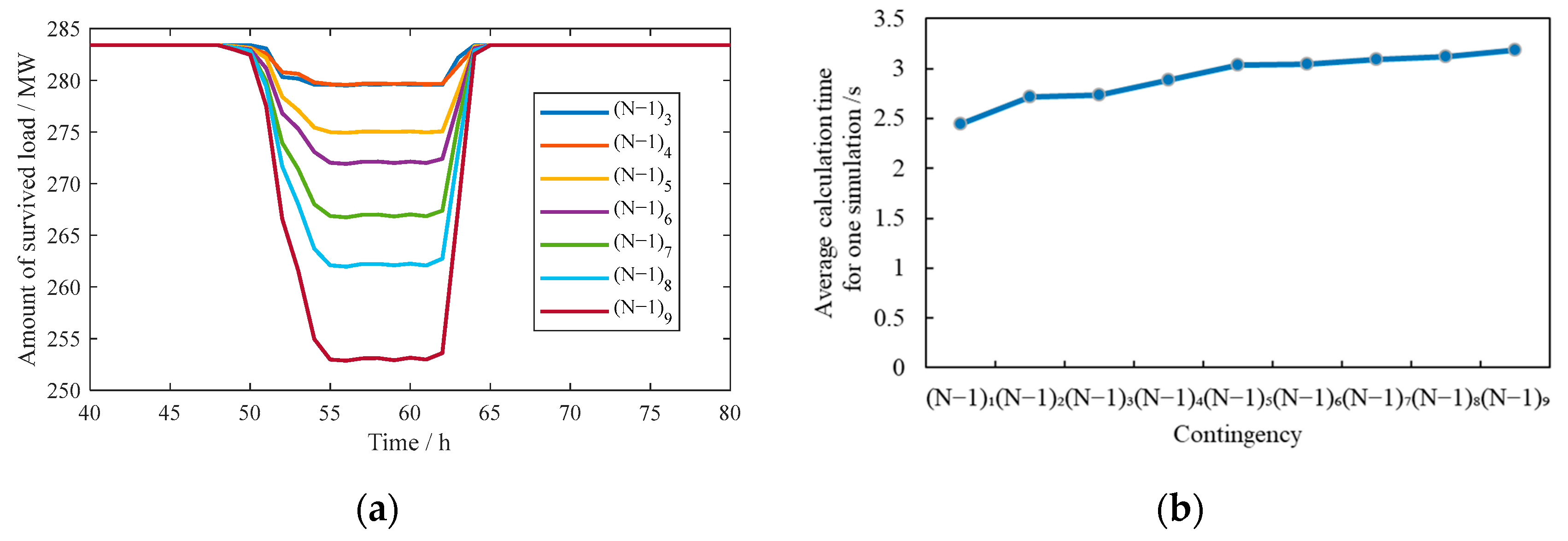
4.4. Impact of Different Design Wind Loads on System Resilience Assessment Results

To verify the effectiveness of the proposed comprehensive system resilience assessment method, various design wind loads are statistically configured to assess the probability of (N − 1)k contingency occurrence. The percentage of (N − 1)k contingency scenarios among all contingency scenarios under the different design wind loads (the ratio of the number of (N − 1)k contingency scenarios to the number of all scenarios in each contingency set) and the CRI under different design wind loads are shown in Figure 10 and Table 5.
It can be seen from Table 5 that when the design wind load is increased from 0.8 to 1.5 times that of the original design wind load W0, the probability of multiple contingencies under the current contingency set will decrease, and the number of contingencies will also decrease. That is, (N − 1)1 contingency is most likely to occur compared with other (N − 1)k contingencies when the design wind load is 1.5 W0; (N − 1)3 contingency is most likely to occur when the design wind load is 1.3 W0; (N − 1)6 contingency is most likely to occur when the design wind load is 1.1 W0; and (N − 1)9 or even higher contingencies are most likely to occur when the design wind load is less than or equal to W0. In addition, the (N − 1)1 and (N − 1)2 contingencies almost do not cause load shedding. Therefore, with the increase in the design wind load, the wind resistance of the components is enhanced, and the system resilience is improved accordingly. At the same time, the regular maintenance and wind-proof reinforcement of lines and towers before the typhoon disasters are conducive to increasing the design wind loads, which can significantly improve the resilience of the power grid.

5. Conclusions

In this paper, a holistic resilience assessment framework considering wind-PV output uncertainty and spatial–temporal failure probability during typhoon extreme weather is proposed and comprehensively evaluated by using EWM and TOPSIS methods. Through the case study, the following conclusions are drawn.
  • The parametric typhoon wind field model has high computational efficiency, and the optimal typhoon wind field model and corresponding parameters can be selected by integrating the typhoon reanalysis data in typhoon-prone regions, which is particularly suitable for engineering applications.
  • The spatial–temporal failure probability model for components based on the stress–strength interference method, as well as the spatial–temporal contingency set considering time series and recovery time, can effectively capture the spatial–temporal impacts of typhoons on the power grid.
  • Extreme typhoon events can lead to (N − 1)k contingencies. The proposed system resilience assessment framework combined with the optimal load shedding strategy considering the load importance is helpful to minimize critical load loss and elucidate the response of the power grid to typhoons with different intensities and multiple contingencies. In addition, the multi-dimensional capabilities of the power grid in the face of extreme typhoon events, such as priority, robustness, rapidity, and sustainability, are evaluated as well.
The typhoon best track data required for the proposed comprehensive resilience assessment framework can be sourced from the typhoon track prediction data released by meteorological departments around the world. The optimal wind field model can be determined by the historical typhoon reanalysis data specific to the region. Therefore, the resilience assessment framework proposed in this paper is of great value for pre-diagnosis in the pre-disaster stage, typhoon disaster warning, pre-study of emergency repair strategies by utilities, and verification of the effectiveness of resilience enhancement strategies. It is worth mentioning that future research on power system resilience assessment based on actual systems and more accurate meteorological information will be more practical. In our future work, the resilience assessment framework proposed in this paper can be further modified by introducing more practical factors to obtain a more applicable, robust, and universal multi-hazard resilience assessment framework. In addition, incorporating more diverse and predictive data sources in resilience assessment research can greatly enhance the emergency and disaster response capabilities of future power grids.

Author Contributions

Conceptualization, W.W. and L.S.; methodology, W.W. and L.S.; software, W.W.; validation, W.W., L.S. and Z.Q.; resources, Z.Q.; writing—original draft preparation, W.W.; writing—review and editing, L.S. All authors have read and agreed to the published version of the manuscript.

Funding

This research was funded by the 2021 Stabilization Support Program (Shenzhen Science and Technology Commission), grant number WDZC20200819174646001.

Data Availability Statement

The datasets generated and analyzed during the current study are available from the corresponding author upon reasonable request.

Conflicts of Interest

The authors declare no conflicts of interest.

References

  1. Che, L.; Khodayar, M.; Shahidehpour, M. Only Connect: Microgrids for Distribution System Restoration. IEEE Power Energy Mag. 2014, 12, 70–81. [Google Scholar] [CrossRef]
  2. Mahzarnia, M.; Parsa Moghaddam, M.; Siano, P.; Haghifam, M.-R. A Comprehensive Assessment of Power System Resilience to a Hurricane Using a Two-Stage Analytical Approach Incorporating Risk-Based Index. Sustain. Energy Technol. Assess. 2020, 42, 100831. [Google Scholar] [CrossRef]
  3. Bie, Z.; Lin, C.; Li, G.; Qiu, A. Development and Prospect of Resilient Power System in the Context of Energy Transition. Proc. Chin. Soc. Electr. Eng. 2020, 40, 2735–2745. (In Chinese) [Google Scholar]
  4. Mlilo, N.; Brown, J.; Ahfock, T. Impact of Intermittent Renewable Energy Generation Penetration on the Power System Networks—A Review. Technol. Econ. Smart Grids Sustain. Energy 2021, 6, 25. [Google Scholar] [CrossRef]
  5. Xu, L.; Feng, K.; Lin, N.; Perera, A.T.D.; Poor, H.V.; Xie, L.; Ji, C.; Sun, X.A.; Guo, Q.; O’Malley, M. Resilience of Renewable Power Systems under Climate Risks. Nat. Rev. Electr. Eng. 2024, 1, 53–66. [Google Scholar] [CrossRef]
  6. Jordehi, A.R.; Tabar, V.S.; Mansouri, S.A.; Sheidaei, F.; Ahmarinejad, A.; Pirouzi, S. Two-Stage Stochastic Programming for Scheduling Microgrids with High Wind Penetration Including Fast Demand Response Providers and Fast-Start Generators. Sustain. Energy Grids Netw. 2022, 31, 100694. [Google Scholar] [CrossRef]
  7. Bie, Z.; Lin, Y.; Li, G.; Li, F. Battling the Extreme: A Study on the Power System Resilience. Proc. IEEE 2017, 105, 1253–1266. [Google Scholar] [CrossRef]
  8. Craig, M.T.; Wohland, J.; Stoop, L.P.; Kies, A.; Pickering, B.; Bloomfield, H.C.; Browell, J.; De Felice, M.; Dent, C.J.; Deroubaix, A.; et al. Overcoming the Disconnect between Energy System and Climate Modeling. Joule 2022, 6, 1405–1417. [Google Scholar] [CrossRef]
  9. Liu, Z.; Xu, L.; Lu, Q. Comprehensive Typhoon Hazard Zoning in China Based on Historical Records. Geomat. Nat. Hazards Risk 2024, 15, 2300813. [Google Scholar] [CrossRef]
  10. Wang, Z.; Wang, Z. A Novel Preventive Islanding Scheme of Power System under Extreme Typhoon Events. Int. J. Electr. Power Energy Syst. 2023, 147, 108857. [Google Scholar] [CrossRef]
  11. Rong, J.; Zhou, M.; Li, G. Resilience-Oriented Restoration Strategy by Offshore Wind Power Considering Risk. CSEE J. Power Energy Syst. 2023, 9, 2052–2065. [Google Scholar] [CrossRef]
  12. Tang, W.; Yang, Y.; Li, Y.; Lu, J.; Wu, Q. Investigation on Resilience Assessment and Enhancement for Power Transmission Systems Under Extreme Meteorological Disasters. Proc. Chin. Soc. Electr. Eng. 2020, 40, 2244–2254+2403. (In Chinese) [Google Scholar] [CrossRef]
  13. Lu, P.; Xu, M.; Sun, A.; Wang, Z.; Zheng, Z. Typhoon Tracks Prediction with ConvLSTM Fused Reanalysis Data. Electronics 2022, 11, 3279. [Google Scholar] [CrossRef]
  14. Gautam, P.; Piya, P.; Karki, R. Resilience Assessment of Distribution Systems Integrated With Distributed Energy Resources. IEEE Trans. Sustain. Energy 2021, 12, 338–348. [Google Scholar] [CrossRef]
  15. Gautam, M.; Ben-Idris, M. Optimal Sizing of Movable Energy Resources for Enhanced Resilience in Distribution Systems: A Techno-Economic Analysis. Electronics 2023, 12, 4256. [Google Scholar] [CrossRef]
  16. Zhang, W.; Shao, C.; Hu, B.; Xie, K.; Siano, P.; Li, M.; Cao, M. Transmission Defense Hardening Against Typhoon Disasters Under Decision-Dependent Uncertainty. IEEE Trans. Power Syst. 2023, 38, 2653–2665. [Google Scholar] [CrossRef]
  17. Watson, E.B.; Etemadi, A.H. Modeling Electrical Grid Resilience Under Hurricane Wind Conditions With Increased Solar and Wind Power Generation. IEEE Trans. Power Syst. 2020, 35, 929–937. [Google Scholar] [CrossRef]
  18. Ceferino, L.; Lin, N.; Xi, D. Stochastic Modeling of Solar Irradiance during Hurricanes. Stoch. Environ. Res. Risk Assess. 2022, 36, 2681–2693. [Google Scholar] [CrossRef]
  19. Zheng, X.; Xie, L.; Lee, K.; Fu, D.; Wu, J. Impact of Climate Simulation Resolutions on Future Energy System Reliability Assessment: A Texas Case Study. iEnergy 2023, 2, 222–230. [Google Scholar] [CrossRef]
  20. Wang, S.; Foley, A.M.; Chen, N.; Chen, B. Risk-Based Dispatch Strategy for a Power System with High Wind Power Integration Considering Damage Due to Typhoons. Electr. Power Compon. Syst. 2023, 51, 2098–2115. [Google Scholar] [CrossRef]
  21. Silva, F.T.d.; Baierle, I.C.; Correa, R.G.d.F.; Sellitto, M.A.; Peres, F.A.P.; Kipper, L.M. Open Innovation in Agribusiness: Barriers and Challenges in the Transition to Agriculture 4.0. Sustainability 2023, 15, 8562. [Google Scholar] [CrossRef]
  22. Gerhardt, V.J.; Mairesse Siluk, J.C.; Baierle, I.C.; Michelin, C. de F. Theoretical Model for Identifying Market Development Indicators. Int. J. Product. Perform. Manag. 2021, 71, 2659–2679. [Google Scholar] [CrossRef]
  23. Wang, Y.; Yang, Y.; Xu, Q. Reliability Assessment for Integrated Power-Gas Systems Considering Renewable Energy Uncertainty and Cascading Effects. CSEE J. Power Energy Syst. 2023, 9, 1214–1226. [Google Scholar] [CrossRef]
  24. Pourdaryaei, A.; Shahriari, A.; Mohammadi, M.; Aghamohammadi, M.R.; Karimi, M.; Kauhaniemi, K. A New Approach for Long-Term Stability Estimation Based on Voltage Profile Assessment for a Power Grid. Energies 2023, 16, 2508. [Google Scholar] [CrossRef]
  25. Zhang, H.; Yuan, H.; Li, G.; Lin, Y. Quantitative Resilience Assessment under a Tri-Stage Framework for Power Systems. Energies 2018, 11, 1427. [Google Scholar] [CrossRef]
  26. Panteli, M.; Trakas, D.N.; Mancarella, P.; Hatziargyriou, N.D. Power Systems Resilience Assessment: Hardening and Smart Operational Enhancement Strategies. Proc. IEEE 2017, 105, 1202–1213. [Google Scholar] [CrossRef]
  27. Panteli, M.; Mancarella, P.; Trakas, D.N.; Kyriakides, E.; Hatziargyriou, N.D. Metrics and Quantification of Operational and Infrastructure Resilience in Power Systems. IEEE Trans. Power Syst. 2017, 32, 4732–4742. [Google Scholar] [CrossRef]
  28. Raoufi, H.; Vahidinasab, V.; Mehran, K. Power Systems Resilience Metrics: A Comprehensive Review of Challenges and Outlook. Sustainability 2020, 12, 9698. [Google Scholar] [CrossRef]
  29. Zhang, H.; Ma, S.; Ding, T.; Lin, Y.; Shahidehpour, M. Multi-Stage Multi-Zone Defender-Attacker-Defender Model for Optimal Resilience Strategy With Distribution Line Hardening and Energy Storage System Deployment. IEEE Trans. Smart Grid 2021, 12, 1194–1205. [Google Scholar] [CrossRef]
  30. Nassif, A.B.; Ericson, S.; Abbey, C.; Jeffers, R.; Hotchkiss, E.; Bahramirad, S. Valuing Resilience Benefits of Microgrids for an Interconnected Island Distribution System. Electronics 2022, 11, 4206. [Google Scholar] [CrossRef]
  31. Yao, D.; Han, J.; Li, Q.; Wang, Q.; Li, C.; Zhang, D.; Li, M.; Tian, C. An Intelligent Risk Forewarning Method for Operation of Power System Considering Multi-Region Extreme Weather Correlation. Electronics 2023, 12, 3487. [Google Scholar] [CrossRef]
  32. Wen, X.; Wu, T.; Wang, H.; Peng, J.; Jiang, H. A Novel Transient Stability Control Strategy for an AC/MTDC Grid Under N-k Contingency Induced by Typhoon Extreme Weather. IEEE Trans. Power Deliv. 2023, 38, 3441–3454. [Google Scholar] [CrossRef]
  33. Yang, Y.; Tang, W.; Liu, Y.; Xin, Y.; Wu, Q. Quantitative Resilience Assessment for Power Transmission Systems Under Typhoon Weather. IEEE Access 2018, 6, 40747–40756. [Google Scholar] [CrossRef]
  34. Amirioun, M.H.; Aminifar, F.; Lesani, H.; Shahidehpour, M. Metrics and Quantitative Framework for Assessing Microgrid Resilience against Windstorms. Int. J. Electr. Power Energy Syst. 2019, 104, 716–723. [Google Scholar] [CrossRef]
  35. Bajpai, P.; Chanda, S.; Srivastava, A.K. A Novel Metric to Quantify and Enable Resilient Distribution System Using Graph Theory and Choquet Integral. IEEE Trans. Smart Grid 2018, 9, 2918–2929. [Google Scholar] [CrossRef]
  36. Zhang, G.; Zhang, F.; Wang, X.; Zhang, X. Fast Resilience Assessment of Distribution Systems With a Non-Simulation-Based Method. IEEE Trans. Power Deliv. 2022, 37, 1088–1099. [Google Scholar] [CrossRef]
  37. Liu, C.; Yu, J.; Zhu, X.; Wang, D.; Guan, X. Global Maximum Flow Based Time-Domain Simulation Method for Evaluating Power System Resilience. Energy Rep. 2023, 9, 532–541. [Google Scholar] [CrossRef]
  38. Dehghani, A.; Sedighizadeh, M.; Haghjoo, F. Defining a New Index to Compare the Resilience of Different Structures of an Electrical Energy Network. IET Gener. Transm. Distrib. 2023, 17, 875–895. [Google Scholar] [CrossRef]
  39. Lu, J.; Guo, J.; Jian, Z.; Yang, Y.; Tang, W. Dynamic Assessment of Resilience of Power Transmission Systems in Ice Disasters. In Proceedings of the 2018 International Conference on Power System Technology (POWERCON), Guangzhou, China, 6–8 November 2018; pp. 7–13. [Google Scholar]
  40. Chang, D.; Amin, S.; Emanuel, K. Modeling and Parameter Estimation of Hurricane Wind Fields with Asymmetry. J. Appl. Meteorol. Climatol. 2020, 59, 687–705. [Google Scholar] [CrossRef]
  41. Wu, Y.; Dou, S.; Fan, Y.; Yu, S.; Dai, W. Research on the Influential Characteristics of Asymmetric Wind Fields on Typhoon Waves. Front. Mar. Sci. 2023, 10, 1113494. [Google Scholar] [CrossRef]
  42. Wang, C.; Zhang, H.; Feng, K.; Li, Q. A Simple Gradient Wind Field Model for Translating Tropical Cyclones. Nat. Hazards 2017, 88, 651–658. [Google Scholar] [CrossRef]
  43. Tian, Z.; Zhang, Y. Numerical Estimation of the Typhoon-Induced Wind and Wave Fields in Taiwan Strait. Ocean. Eng. 2021, 239, 109803. [Google Scholar] [CrossRef]
  44. Willoughby, H.E.; Rahn, M.E. Parametric Representation of the Primary Hurricane Vortex. Part I: Observations and Evaluation of the Holland (1980) Model. Mon. Weather Rev. 2004, 132, 3033–3048. [Google Scholar] [CrossRef]
  45. Batts, M.E.; Simiu, E.; Russell, L.R. Hurricane Wind Speeds in the United States. J. Struct. Div. 1980, 106, 2001–2016. [Google Scholar] [CrossRef]
  46. Mitsuta, Y.; Fujii, T. Analysis and Synthesis of Typhoon Wind Pattern over Japan. Bull. Disaster Prev. Res. Inst. 1987, 37, 169–185. [Google Scholar]
  47. Jelesnianski, C.; Chen, J.; Shaffer, W. SLOSH: Sea, Lake, and Overland Surges from Hurricanes; US Department of Commerce; National Oceanic and Atmospheric Administration; National Weather Service: Silver Spring, MD, USA, 1992.
  48. Jelesnianski, C.P. Numerical computations of storm surges without bottom stress. Mon. Weather Rev. 1966, 94, 379–394. [Google Scholar] [CrossRef]
  49. Holland, G.J. An Analytic Model of the Wind and Pressure Profiles in Hurricanes. Mon. Weather Rev. 1980, 108, 1212–1218. [Google Scholar] [CrossRef]
  50. Miyazaki, M. Theoretical Investigations of Typhoon Surges along the Japanese Coast (II).: Miyazaki, M., T. Ueno, and S. Unoki, 1962. Oceanogr. Mag., 13 (2): 103–118. Deep. Sea Res. Oceanogr. Abstr. 1963, 10, 347. [Google Scholar] [CrossRef]
  51. Liu, R.; Ming, J. Comparative analysis of the characteristics of the tropical cyclone sea surface inflow angle and drag coefficient in the Atlantic and the Western Pacific oceans. Chin. J. Geophys. Chin. Ed. 2021, 64, 2579–2589. [Google Scholar] [CrossRef]
  52. Meng, Y.; Matsui, M.; Hibi, K. A Numerical Study of the Wind Field in a Typhoon Boundary Layer. J. Wind. Eng. Ind. Aerodyn. 1997, 67, 437–448. [Google Scholar] [CrossRef]
  53. Harper, B.A.; Kepert, J.D.; Ginger, J.D. Guidelines for Converting between Various Wind Averaging Periods in Tropical Cyclone Conditions; WMO/TD-No. 1555; World Meteorological Organization: Geneva, Switzerland, 2010. [Google Scholar]
  54. Sun, W.; Zamani, M.; Hesamzadeh, M.R.; Zhang, H.-T. Data-Driven Probabilistic Optimal Power Flow With Nonparametric Bayesian Modeling and Inference. IEEE Trans. Smart Grid 2020, 11, 1077–1090. [Google Scholar] [CrossRef]
  55. Dai, L.; You, D.; Yin, X. Data Driven Robust Energy and Reserve Dispatch Based on a Nonparametric Dirichlet Process Gaussian Mixture Model. Energies 2020, 13, 4642. [Google Scholar] [CrossRef]
  56. GB 50545-2010; Code for Design of 110–750 kV Overhead Transmission Line. China Planning Press: Beijing, China, 2010.
  57. IEC 60826:2017; Design Criteria of Overhead Transmission Lines. International Electrotechnical Commission: Geneva, Switzerland, 2017.
  58. Pakdaman, Z.; Shekari, M.; Zamani, H. Stress-Strength Reliability of a Failure Profile with Components Operating under the Internal Environmental Factors. Int. J. Reliab. Qual. Saf. Eng. 2023, 30, 2350019. [Google Scholar] [CrossRef]
  59. Zimmerman, R.D.; Murillo-Sánchez, C.E.; Thomas, R.J. MATPOWER: Steady-State Operations, Planning, and Analysis Tools for Power Systems Research and Education. IEEE Trans. Power Syst. 2011, 26, 12–19. [Google Scholar] [CrossRef]
  60. Cheng, Q.Y. Structure Entropy Weight Method to Confirm the Weight of Evaluating Index. Syst. Eng. Theory Pract. 2010, 30, 1225–1228. [Google Scholar]
  61. Shih, H.-S.; Shyur, H.-J.; Lee, E.S. An Extension of TOPSIS for Group Decision Making. Math. Comput. Model. 2007, 45, 801–813. [Google Scholar] [CrossRef]
  62. Zhang, Y.Q.; Xu, Z.; Yu, H.H.; Qiu, Z.X. Study on Practical Probability Density Function of Solar Irradiation in Multi-orientations. Acta Energiae Solaris Sin. 2022, 43, 132–139. (In Chinese) [Google Scholar] [CrossRef]
  63. Xu, Z.; Hu, X.Y.; Chen, Q.; Qiu, Z.X. Measurement and Study of Solar Energy Resource in Different Orientations. Acta Energiae Solaris Sin. 2016, 37, 891–896. (In Chinese) [Google Scholar]
Figure 1. The holistic research framework.
Electronics 13 00745 g001
Figure 2. Schematic diagram of component actual wind load and design wind load interference.
Electronics 13 00745 g002
Figure 3. Schematic diagram of resilience indicators.
Electronics 13 00745 g003
Figure 4. Flow chart of the comprehensive resilience assessment framework solution.
Electronics 13 00745 g004
Figure 5. (a) The geographical wiring diagram of the improved IEEE-30 bus test system; (b) the single-line diagram of the improved IEEE-30 bus test system.
Electronics 13 00745 g005
Figure 6. (a) Comparisons between meteorological observed values and wind field simulations of Typhoon Mangkhut; (b) comparisons between typhoon meteorological observed values and wind field simulations of Typhoon Nida; (c) comparisons between typhoon meteorological observed values and wind field simulations of Typhoon Merbok.
Electronics 13 00745 g006
Figure 7. Typical wind-PV output scenarios during Typhoon Mangkhut.
Electronics 13 00745 g007
Figure 8. (a) Failure probability of all 41 lines during Typhoon Mangkhut; (b) the expected amount of survived load during Typhoon Mangkhut; (c) curves of the expected amount of survived load in the face of typhoons with different intensities.
Electronics 13 00745 g008
Figure 9. (a) The amount of survived load for (N − 1)k contingencies caused by Typhoon Mangkhut; (b) average calculation time for one simulation of (N − 1)k contingencies.
Electronics 13 00745 g009
Figure 10. (a) Percentage of (N − 1)k contingency under different design wind loads; (b) curves of the amount of survived load.
Electronics 13 00745 g010
Table 1. Some crucial resilience indicators.
CharacteristicMeaning of IndicatorIndicatorFormula
PriorityExtent of disaster impact on critical loadsCritical load shedding ratio R 1 = i 3 ε i P L C , i P L C
RobustnessExtent of system capacity to withstand disastersLoad shedding area R 2 = t = 1 T i = 1 3 P L C , i , t
Maximum amount of load shedding R 3 = max ( P L C , t )
RapidityExtent of rate of load loss and recoveryLoad loss time R 4 = t 2 t 1
Load recovery time R 5 = t 4 t 3
SustainabilityDuration of the whole power outageDuration of load shedding R 6 = t 4 t 1
Table 2. Evaluation metrics of simulation results for different typhoons.
TyphoonMetricBattsSchloemerJelenianskiHolland
MangkhutRMSE (m/s)5.65293.82286.93506.2127
MAX (m/s)13.61397.789112.969312.1958
CORR0.84840.89040.95960.8314
NidaRMSE (m/s)3.83078.29244.04665.3877
MAX (m/s)10.340216.457412.410719.2329
CORR0.82440.85910.85980.8952
MerbokRMSE (m/s)3.90937.87965.02396.5380
MAX (m/s)9.754415.363111.710115.6131
CORR0.63000.65300.76480.7739
Table 3. The ten lines with the top 10 failure probability.
NumberLine NumberFailure Probability
1220.3294
2300.3066
3230.2895
4250.2734
5190.2727
6240.2726
7150.2592
810.2540
9180.2516
1040.2493
Table 4. System resilience indicators under different typhoon conditions.
Typhoon ConditionR1R2 (MW·h)R3 (MW)R4 (h)R5 (h)R6 (h)CRI
Typhoon Mangkhut1.7969235.832921.624973160.3826
Typhoon Nida1.859560.47664.956753170.4267
Typhoon Merbok10010001
Table 5. Percentage of (N − 1)k contingency and CRI under different design wind loads.
Wind Load
(kN)
(N − 1)1(N − 1)2(N − 1)3(N − 1)4(N − 1)5(N − 1)6(N − 1)7(N − 1)8(N − 1)9CRI
0.8 W000000.00210.01650.05990.26650.65500.1554
0.9 W00000.00590.01380.06480.13560.29470.48530.2405
W0000.00180.01320.04750.09910.18870.28510.36460.2749
1.1 W00.00510.02050.06600.12220.18740.20260.17740.13570.08310.3276
1.2 W00.03110.10250.17100.22430.19240.14280.08190.04520.00890.3517
1.3 W00.10540.22520.25580.21360.11530.06030.01780.00540.00120.3942
1.4 W00.26870.30550.23460.12650.04730.01530.0022000.4009
1.5 W00.41060.33850.17880.05340.01710.00150000.4164
Disclaimer/Publisher’s Note: The statements, opinions and data contained in all publications are solely those of the individual author(s) and contributor(s) and not of MDPI and/or the editor(s). MDPI and/or the editor(s) disclaim responsibility for any injury to people or property resulting from any ideas, methods, instructions or products referred to in the content.

