A Comprehensive Analysis of PINNs for Power System Transient Stability

Abstract

The integration of machine learning in power systems, particularly in stability and dynamics, addresses the challenges brought by the integration of renewable energies and distributed energy resources (DERs). Traditional methods for power system transient stability, involving solving differential equations with computational techniques, face limitations due to their time-consuming and computationally demanding nature. This paper introduces physics-informed Neural Networks (PINNs) as a promising solution for these challenges, especially in scenarios with limited data availability and the need for high computational speed. PINNs offer a novel approach for complex power systems by incorporating additional equations and adapting to various system scales, from a single bus to multi-bus networks. Our study presents the first comprehensive evaluation of physics-informed Neural Networks (PINNs) in the context of power system transient stability, addressing various grid complexities. Additionally, we introduce a novel approach for adjusting loss weights to improve the adaptability of PINNs to diverse systems. Our experimental findings reveal that PINNs can be efficiently scaled while maintaining high accuracy. Furthermore, these results suggest that PINNs significantly outperform the traditional ode45 method in terms of efficiency, especially as the system size increases, showcasing a progressive speed advantage over ode45.

1. Introduction

The use of machine learning in power systems, particularly in the realms of power system stability and dynamics, is not a new concept in the field [1]. In recent years, the integration of renewable energies and the incorporation of distributed energy resources (DERs) have led to significant transformations in power systems [2,3,4]. These changes have raised serious concerns about system security and stability, as they introduce variability and necessitate precise simulations of transients. The conventional view of networks as passive entities is no longer viable. Consequently, there is an increasing demand for the development of simulation tools that can accurately capture these transients, enabling comprehensive stability studies and ensuring system reliability [5].

Traditionally, power system transient stability was addressed using standard scientific computational methods; the primary challenge involved solving differential equations using various numerical methods as approximations to obtain accurate solutions [6,7]. Typically, ordinary differential equations (ODEs) were solved using computational techniques such as the Euler, Adams, Runge–Kutta, and Newton–Raphson methods. Partial differential equations (PDEs) were usually tackled using mathematical methods like finite difference, finite element, finite volume, and (pseudo-)spectral methods [8,9,10,11,12,13,14,15]. Recently, researchers have employed some advanced mathematical techniques [16,17]. While these methods are highly accurate, they are often time-consuming and computationally demanding. This becomes a critical concern with the transition to unpredictable and rapidly changing sources like renewable energy, where increased variability leads to sharp and fast transients, making simulations more complex. Therefore, the primary focus of this paper is to find new simulation tools capable of efficiently handling these challenges, with an emphasis on flexibility and speed to meet current demands.

Various data-driven approaches have been explored in the context of power systems. A review of more data-driven approaches is available in [1], with specific examples in [18,19]. Traditional data-driven techniques excel in scenarios where speed is essential and ample data are available, especially when applied to energy systems [20,21,22]. These methods have faster inference speeds compared to traditional computational methods. However, they have fundamental limitations: (1) they require significant amounts of data; (2) the data might be polluted, leading to unrealistic physical models; and (3) predicting corner cases can be challenging.

One solution to these limitations is building a direct connection to the underlying physical principles. Thankfully, advancements in computational capabilities [23] and automatic differentiation methods [24] have successfully bridged the gap between data-driven approaches and a comprehensive understanding of the underlying physical problems. This integration of physics-based knowledge into machine learning algorithms has improved accuracy and reliability in the models employed. Figure 1 shows a representation of this new scientific machine learning approach: physics-informed Neural Networks (PINNs).

In scenarios where only limited data are available, computational speed is crucial, and when there is a solid understanding of the underlying theoretical model, the application of physics-informed Neural Networks (PINNs) emerges as a promising approach for tackling differential equations in power system transient stability. Particularly for complex multiple-bus power systems, PINNs offer an appealing alternative by leveraging their flexibility to incorporate additional equations, thereby benefiting large-scale systems. Unlike traditional methods, PINNs utilize direct function mapping for notably swift inference processes, and they do not require extensive datasets, distinguishing them in the field. These concepts have been explored in the literature, with Ref. [25] presenting an example of employing PINNs in converter dynamics, and Refs. [26,27] demonstrating their application in rotor angle stability. A comprehensive review of PINNs in power system stability was developed in [28].

Previous research has explored the application of PINNs in power systems, but no comprehensive evaluation has been conducted to date. In our study, we pioneer an in-depth analysis of physics-informed Neural Networks (PINNs) in the realm of power system transient stability, exploring their application across a spectrum of grid complexities. This marks the first endeavor of its kind. Our research ambitiously extends across power systems of varying scales, from single-bus systems to intricate 14-bus networks, and from configurations with a single generator to those incorporating five generators. A significant finding is that PINNs maintain their scalability without any loss in accuracy, even as system complexity increases. This insight demonstrates the robustness of PINNs in diverse settings. Furthermore, we introduce a revolutionary method for adjusting loss weights, enhancing the adaptability of PINNs to a wide range of systems. Additionally, our research includes a meticulous evaluation of several metrics, providing a comprehensive understanding of their impact on the performance of PINNs in complex power systems. Through this holistic approach, our study aims to illuminate the broader applicability and performance implications of PINNs in diverse power system environments.

The remainder of this paper is organized as follows: Section 2 introduces related works. Section 3 provides a detailed explanation of the construction of the power system case, the database, and the specific considerations for applying physics-informed Neural Networks (PINNs) in power systems. Section 5 presents an analysis of the four simulation cases along with their corresponding results. Furthermore, we delve into a thorough discussion of optimal neural network tuning strategies, considering the scalability of power systems. Finally, Section 6 concludes the paper and outlines future research directions based on our findings.

2. Related Works

Recent literature highlights the diverse applications of physics-informed Neural Networks (PINNs) in power system transient stability, with a particular focus on the ordinary differential equation (ODE) swing equation. These applications vary from simple setups involving a single infinite bus [26] to more intricate configurations involving nine buses [29], all examining rotor angle behavior in synchronous generators. However, there is a noticeable lack of comprehensive analyses of PINNs across different scales of power systems. Further implementation in systems of varying scales is essential to fully ascertain and validate their effectiveness. Moreover, recent studies have investigated model reduction techniques for power system transient stability at the transmission level using partial differential equations (PDEs) [30]. This approach provides a more detailed representation of system dynamics compared to ODEs and offers a promising direction for future research, potentially serving as an alternative for investigating transient stability in power systems. It is important to recognize, though, that the ODE version of the swing equation remains vital for understanding power system transient stability.

This paper also explores a key advantage of PINNs over traditional computational methods: their effective scalability. Scalability can be assessed in two primary ways: by increasing the number of buses and generators or by broadening the input dimensionality, which includes varying the number and range of input variables. Of these methods, increasing the number of buses has shown significant potential (as evidenced in [29]), while expanding input dimensionality poses more challenges and is yet to be conclusively proven. Another novel approach to scalability is the use of graphical neural networks, specifically physics-informed graphical networks, which solve complex problems by integrating system physics into graph nodes [31,32].

Additionally, this paper investigates the unique flexibility of PINNs compared to other methods. PINNs have recently shown advantages in employing “transfer learning”, allowing adjustments to the power system topology with minimal changes to the differential equations in the neural network. This method considerably reduces training time and yields more effective solutions by incorporating a theoretical model through the loss function [33,34,35]. PINNs have also proven effective in addressing variable initial conditions, as demonstrated in reference [36].

Conversely, a primary challenge for PINNs lies in handling sharp solution transitions, often due to imbalances in the neural network’s loss function. In electrical power systems, such abrupt changes may occur during events like power blackouts affecting the grid or the integration of renewable energies. To tackle these nonlinearities, a novel method involving PINNs with adaptive localized artificial viscosity was proposed in [37]. This approach balances theoretical and data-driven losses in a PINN, enabling more effective management of sharp transients. Further strategies to adjust loss imbalance were discussed in [38,39], inspiring the new method introduced in this paper.

In summary, this paper focuses exclusively on using PINNs to address the ODE swing equation for rotor angle stability in various bus systems, thoroughly assessing their effectiveness in power system transient stability across a range of scales.

3. Power System Transient Stability and Swing Equations

Power system stability is a critical aspect that concerns the system’s ability to maintain a balanced and steady state, not only during routine operations but also following sudden disturbances. One particular aspect of this stability is transient stability, which focuses on the system’s ability to recover and regain its stable operational state after unexpected events such as load changes, faults, or the loss of generators. To analyze transient stability in greater detail, engineers often rely on the swing equation. This equation is a fundamental model for examining the behavior of three-phase synchronous generators under transient conditions. It essentially captures the dynamics of rotor angles, offering a simplified yet insightful view of the system’s response, particularly during the initial stages of stability analysis. Although the swing equation might not provide the most precise results due to its inherent simplifications, it remains a valuable tool for gaining preliminary insights into how a power system will respond to disruptions. The swing equation, as indicated by (1) and (2), is used to simulate the behavior of rotor angles ${\delta }_i$ for the i-th generator:

$${\displaystyle \frac{d{\delta }_i}{dt}}=w_i-w_0,$$

(1)

$${\displaystyle \frac{d^2{\delta }_i}{d{t}^2}}={\displaystyle \frac{w_0}{2H_i}}(P_{mi}-P_{ei}-D_i\frac{d{\delta }_i}{dt}),$$

(2)

where $w_i$ represents the electrical radian frequency, while $w_0$ stands for the synchronous electrical radian frequency. $P_{ei}$ signifies the electrical power output of the generator, accounting for electrical losses. Conversely, $P_{mi}$ refers to the mechanical power supplied by the prime mover, after subtracting mechanical losses, all expressed per unit. $D_i$ is the damping constant, and $H_i$ is the normalized inertia constant, as cited in [8]. To compute the electrical power at each bus $P_{ei}$ from (2), we have to solve the power flow problem represented by (3):

$$P_{ei}=V_i\sum _{n=1}^N{b}_{in}{V}_{n}cos({\theta }_i-{\theta }_n-{\theta }_{Y_{in}})+P_{li},$$

(3)

where the variable $b_{in}$ refers to the susceptance matrix of the system, while ${\theta }_i$, ${\theta }_n$, and ${\theta }_{Y_{in}}$ represent the power angles at buses i and n and the corresponding impedance angle of the transmission line, respectively. The variables $V_i$ and $P_{li}$ represent the voltage magnitude and the load at each bus, respectively. Additionally, establishing the connection between the power angle $\theta$ and the rotor angle $\delta$ is crucial. The synchronous generator model shown in Figure 2 demonstrates this link, which hinges on the generator’s internal inductance X. This model explicates how the power angle $\theta$ at a specific bus, the site of the generator, correlates with the rotor angle $\delta$.

On the other hand, (4) calculates the power angle at a specific bus where no generator is present, and the dynamics of the load determine the evolution of the power angle [29]. To maintain consistent notation throughout the paper, we will represent the power angle $\delta$ as $\theta$ at the buses where only loads are connected in all subsequent discussions.

$${\displaystyle \frac{d{\theta }_i}{dt}}=-{\displaystyle \frac{P_{ei}}{D_i}}.$$

(4)

By employing this approach, we are able to simulate the dynamic behavior of the rotor angles for each generator within the system, as well as the dynamics of the power angles at the buses where only loads are connected.

4. Method: PINNs on Power Systems

In this section, we explore the architecture and methodology of physics-informed Neural Networks (PINNs) in power systems. As shown in Figure 3, PINNs are similar to conventional neural networks, which consist of four main components: the input, the mapping represented by neural networks, the output, and the loss function. However, there are significant differences in these four components in PINNs compared to those in conventional neural networks. The input is divided into two distinct terms: one is data-driven, while the other is derived from a theoretical physical model, defined by ODEs/PDEs. In the data-driven part, $x_u$ and $t_u$ are power and time data samples from initial/boundary conditions, respectively, and u corresponds to the ground truth of $(x_u,t_u)$. The variables $x_f$ and $t_f$ represent the power and time, respectively, in the general region for a set of points $N_f$ within the domain. These points are validated by the theoretical physical model, specifically the swing equation of the system. By incorporating this theoretical loss term, the need for additional data u is eliminated, allowing the differential equations to be used instead.

The set of ODEs for each bus representing both the generator and the load dynamics will be denoted as $f\left(x\right)$, following the formulation presented in (5). This formulation aligns with our observations from (1) and (2). The domain of these ODEs, denoted as $\mathrm{\Omega }=(0,T]\times [0,P]$, corresponds to the time t and input mechanical power $P_{mi}$ ranges specified in the dataset subsection.

$$f\left(x\right)=\left\{\begin{array}{cc}{\displaystyle \frac{2H_i}{w_0}}{\displaystyle \frac{d^2{\delta }_i}{d{t}^2}}+P_{ei}+D_i\frac{d{\delta }_i}{dt}-P_{mi}\hfill & \mathrm{if}i=\mathrm{generator}\hfill \\ \\ {\displaystyle \frac{d{\theta }_i}{dt}}-{\displaystyle \frac{P_{ei}}{D_i}}\hfill & \mathrm{if}i=\mathrm{load}\hfill \end{array}\right.$$

(5)

PINNs only rely on some data along with theoretical information obtained from known differential equations. Notably, the neural network only requires boundary and initial condition data for its training process. (6) defines the three crucial terms for generating the training data: the first term corresponds to the initial condition data, while the second and third terms refer to the boundary condition data. The final output of our model $u\left(x\right)$ will represent the corresponding rotor angles throughout the entire domain $x\in [0,T]\times [0,P]$.

$$\beta \left(u\left(x\right)\right)=g\left(x\right)=\left\{\begin{array}{cc}f\left(x\right)\hfill & x\in 0\times [0,P]\hfill \\ f\left(x\right)\hfill & x\in [0,T]\times \left\{0\right\}\hfill \\ f\left(x\right)\hfill & x\in [0,T]\times \left\{P\right\}\hfill \end{array}\right.$$

(6)

For the initial condition data, $f\left(x\right)$ will be governed by (5) at all $P_m$ points when t is equal to zero. As for the boundary condition data, when P equals 0, $f\left(x\right)$ will also be zero; whereas when P equals 1.51, $f\left(x\right)$ will follow (5) with $P_m$ fixed at 1.51. This corresponds to the first term of the loss function referenced in (7) representing the data-driven component of the neural network. Overall, the ultimate objective of the neural network is to discover the most suitable $\theta$ parameters while aiming to minimize a specific loss function:

$${\mathcal{L}}_{MSE}={\mathcal{L}}_{MSE,u}+{\mathcal{L}}_{MSE,f}=\frac{1}{N_u}\sum _{i=1}^{N_u}{\left|u\left(t_u^i,x_u^i\right)-{\overline{u}}^i\right|}^2+\frac{1}{N_f}\sum _{j=1}^{N_f}{\left|f\left(t_f^j,x_f^j\right)\right|}^2.$$

(7)

In the equation denoted by (7), the first term encapsulates data from the initial condition, characterized by the known ground truth ${\overline{u}}^i$. This component signifies the supervised aspect of the training process. Conversely, the second term mandates the differential equation f to equate to zero, representing the unsupervised segment of training that integrates the theoretical foundations of the neural network.

Additionally, another interesting aspect involves the adjustment of weights for these two losses. (8) introduces an additional term ${\lambda }_f$ to adjust the weight of the differential loss component within the overall neural network loss. This methodology will be used in Section 5.3 and Section 5.4 to properly tune our neural networks.

$${\mathcal{L}}_{MSE}={\mathcal{L}}_{MSE,u}+{\lambda }_f{\mathcal{L}}_{MSE,f}.$$

(8)

One of the main challenges in adjusting a physics-informed Neural Network (PINN) is determining the optimal weighting of the losses (${\lambda }_f$ from Equation (8)) to achieve the desired solution. When working with ordinary differential equations (ODEs) or partial differential equations (PDEs), it is well-known that without appropriate boundaries or initial conditions, these equations can have infinitely many solutions. Therefore, it is crucial to ensure that the magnitudes of the gradients of both $Los{s}_u$ (representing the boundary condition loss) and $Los{s}_f$ (representing the differential equation loss) are properly balanced. Failure to achieve this balance may lead the neural network to learn solutions that satisfy the equation but do not accurately represent the desired outcomes. This behavior was observed during the experiments and highlighted the importance of precisely adjusting both loss functions to implement PINNs in power system stability [37,38,39].

Initially, the adjustment of these losses relied on a trial-and-error technique. We experimented with different values of ${\lambda }_f$, namely 1, 0.01, 0.001, and 0.0001, for the 1-bus, 3-bus, 6-bus, and 14-bus power systems, respectively, in Section 5.3 and Section 5.4. While a correlation between the value of ${\lambda }_f$ and the size of the power system was observed, this relationship proved insufficiently accurate for extrapolation to larger systems or systems with different boundary conditions.

Fortunately, based on a method proposed in [38], we implemented a more effective approach for appropriately adjusting these losses, which yielded successful results across all tested scenarios in Section 5.5. The key is to update the parameters of the neural network $\theta$ (i.e., the weights and biases of the neural network) through a gradient-based update algorithm:

$${\widehat{\lambda }}_u=\frac{\overline{\left|{\nabla }_{\theta }{\mathcal{L}}_f\left({\theta }_n\right)\right|}}{\overline{\left|{\nabla }_{\theta }{\mathcal{L}}_u\left({\theta }_n\right)\right|}}.$$

(9)

At the n-th iteration, ${\theta }_n$ represents the parameters of the neural network. The expression $\overline{\left|{\nabla }_{\theta }{\mathcal{L}}_f\left({\theta }_n\right)\right|}$ denotes the mean absolute value of the differential operator for the differential equation loss and $\overline{\left|{\nabla }_{\theta }{\mathcal{L}}_u\left({\theta }_n\right)\right|}$ represents the mean absolute value of the differential operator for the initial condition loss. The logic underlying (9) revolves around determining the relative significance in updating the model between the second and the first loss terms. To achieve a balance between these two loss terms, it is necessary to amplify the first loss term when (9) yields a high value and, conversely, to decrease it when (9) is low. This new weight value should be updated according to penalty term (10) with a recommended value for $\alpha$ of 0.1:

$${\lambda }_u=(1-\alpha ){\lambda }_u+\alpha {\widehat{\lambda }}_u.$$

(10)

Thus, the overall loss of the PINN can be represented by (11), where the new parameter ${\lambda }_u$ is introduced to effectively balance the influence of both individual losses:

$$\mathcal{L}\left(\theta \right)={\lambda }_u{\mathcal{L}}_u\left(\theta \right)+{\mathcal{L}}_f\left(\theta \right).$$

(11)

As previously mentioned, Section 5.5 will report an ablation study using the auto-updated weight method presented above. In the simulations, we set the $N_u$ hyperparameter to 100 and $N_f$ to 15,000. The chosen optimizer was Adam, with a learning rate of 5 $\times {10}^{-3}$. The maximum number of fixed iterations was 5000, 7500, and 10,000 for the 3-bus, 6-bus, and 14-bus power systems, respectively.

5. Results

The proposed physics-informed Neural Network (PINN) was evaluated across various scenarios featuring an increasing number of buses and generators. Specifically, this project investigated four distinct scenarios: infinite-bus, three-bus, six-bus, and fourteen-bus configurations. We validated our method by comparing it with results obtained from the ode45 solver, which we considered the ground truth. The error calculation involved using the ${\mathsf{\ell }}_2$ norm to quantify the difference between the ground truth and the predictions made by the PINNs. This final error metric was derived by aggregating the errors across various buses and then dividing by the total number of buses.

5.1. Dataset

The dataset used in this paper was created using Matlab (R2020a, by MathWorks, Natick, MA, USA). Two different files were developed: one for the PINN in a single-generator system and another for the PINN in multi-generator power systems. The first file focused solely on the simplest scenario, while the second generated a comprehensive dataset covering three different bus systems. The Matlab ode45 solver was used to solve the set of differential equations in all cases.

All systems follow the same methodology: At the n-th bus of the system, there is always a load (or an infinite bus in the simplest case). This load undergoes a unit step function, transitioning from 0.51 to 1.51 per unit (p.u.), resulting in a corresponding increase in generated power at the slack bus, always located at bus 1. This is feasible as long as the resistance of the lines is ignored. The power system experiences a transient period, which was simulated using the Matlab ode45 solver. This allowed us to record the evolution of the rotor angles of the generators and the power angles of the buses where only loads were connected. To simplify the simulation, we assumed the magnitudes of the internal machine voltages E and the internal machine currents I to be constant. A summary of this methodology is illustrated in Figure 4 for each power bus system scenario.

In this research, we conducted simulations for a comprehensive set of 100 cases, exploring a power range from 0.51 to 1.51 per unit (p.u.) both at the n-th bus where the load was located and the slack where a generator was placed. The simulations were performed with a time step consisting of 201 values, covering a time span from 0 to n seconds. Again, n corresponds to the total number of buses present in the system. Thus, the larger the system, the larger the range of the span simulation time. These simulations provided valuable insights and analysis for further understanding and optimizing the system’s behavior under varying power and time conditions.

5.2. Problem Setting

The schematic for each scenario is depicted below:

• One-Bus Power System
  The system was initially turned off, and the load was considered an infinite bus. Figure 5 depicts this first case of study. The inertia constant $H_1$ was equal to 80 p.u., and the damping constant $D_1$ to 1 p.u. Both the line and internal generator reactance were equal to 0.1j.
  The goal of this system was to test the simplest case that the PINN could handle to provide some useful insight into how to tackle more complex systems.
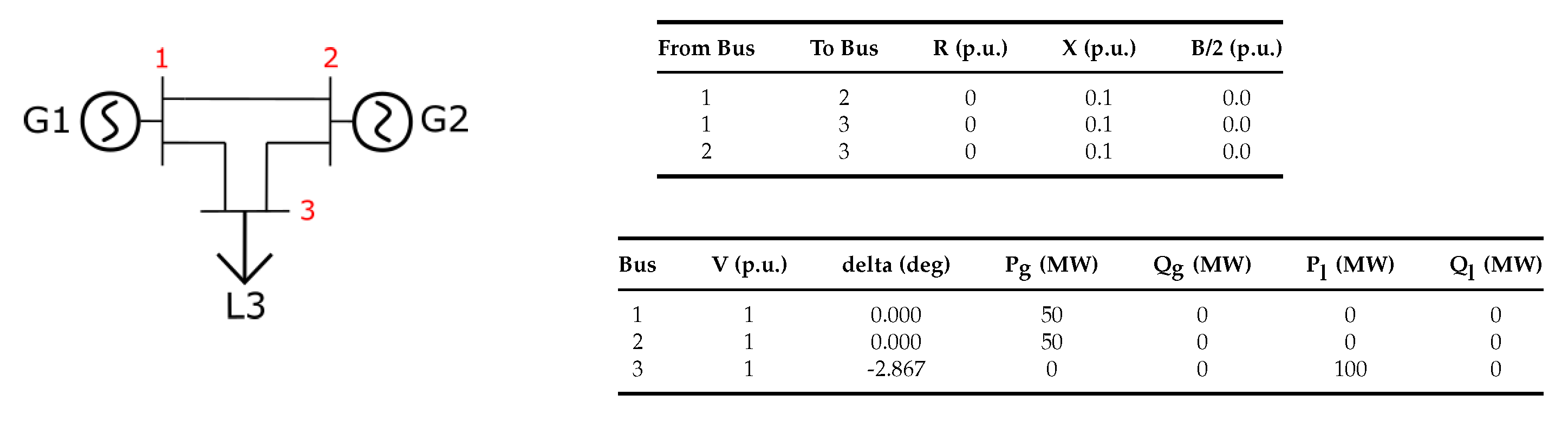
• Three-bus Power System
  The increase in difficulty was achieved by introducing an additional generator into the system. Furthermore, the presence of a load was accounted for using (4). Following the initial examination of the simple one-bus system, this represented the first step towards assessing the scalability of the PINNs. Figure 6 presents a schematic of the three-bus power system in addition to the line data employed and a summary of the chosen initial conditions.
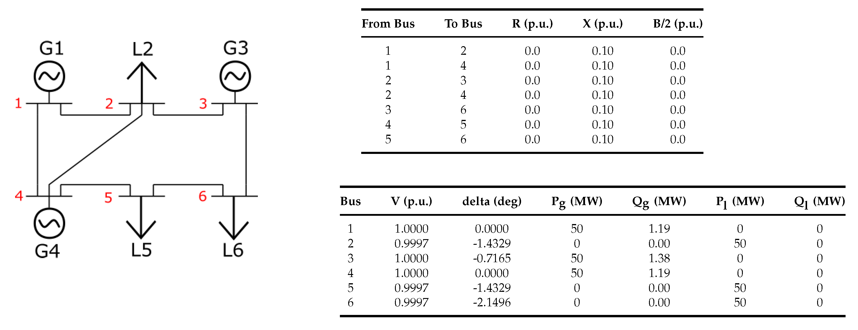
• Six-bus Power System
  The six-bus system scenario is represented in Figure 7. One extra generator and two extra loads were added to test the increased scalability of the PINNs. Figure 7 also presents the line data employed in the six-bus system and a summary of the chosen initial conditions.
• Fourteen-bus Power System
  The last bus system comprised 14 buses, with a total of five generators and nine loads. This system, considered the most intricate in the scope of this paper, is believed to offer abundant data, allowing for the extrapolation of comparable results in larger systems.
  Figure 8 depicts the 14-bus system. Again, the line data were simplified to ease the experimental process, though similar results could be obtained by changing X and $B/2$ to different zero values. The line data employed in the 14-bus system and a summary of the chosen initial conditions are also provided.

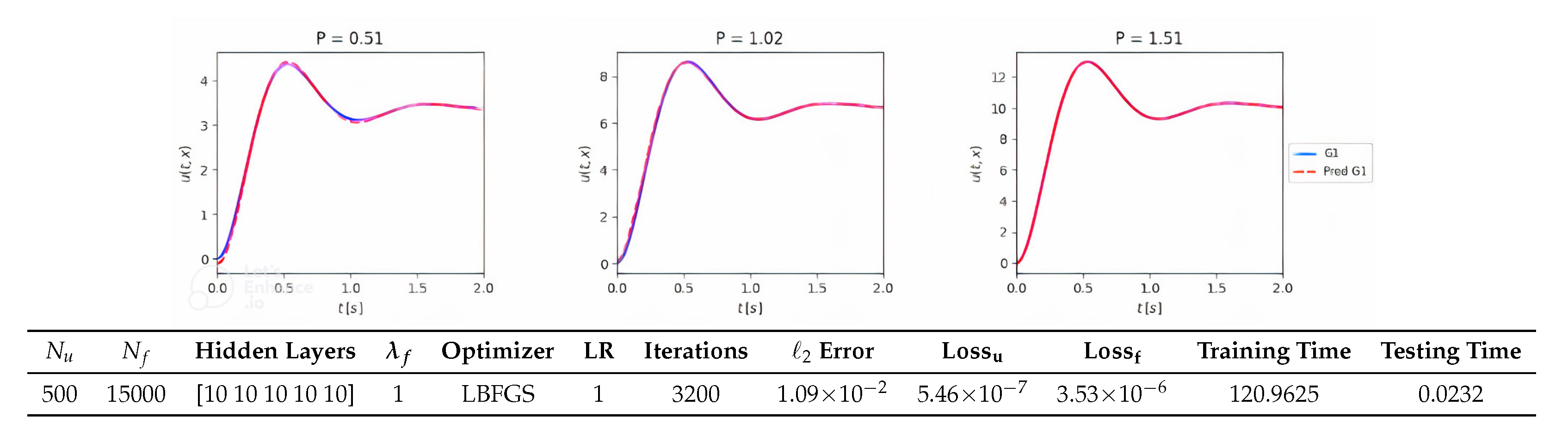
5.3. PINNs on One-Bus System

The simplest model for power system dynamics can be represented by a single machine and an infinite-bus system. This system was already analyzed by [26] and can provide some interesting insights about the behavior in future scalable scenarios.

The testing time of the physics-informed Neural Network was 0.0232 s, which can be compared with the average computational time of 0.1512 s for solving all the differential equations using ode45. The neural network demonstrated more than five-times faster computational speed. The next section will discuss whether this difference increased for larger systems with more buses.

The parameters employed for the best scenario identified are included in Figure 9. Although the number of $N_u$ could be significantly reduced, even with only 50 boundary condition points, we could achieve decent results with reduced training time. However, the ${\mathsf{\ell }}_2$ error increased. In this regard, it is advisable to employ a relatively large number of initial condition points for higher accuracy in the one-bus system case. Other optimization algorithms such as Adam or SGD can also be considered, yielding similar results in this particular case. There is no need to weight any of the losses for this simpler scenario either.

5.4. PINNs on Larger Power Systems

This section provides an analysis of the remaining three power bus systems. Figure 10 depicts the analysis of the three-bus power system utilizing a PINN, with a specific set of parameters that yielded good results. One notable change was the weighting of ${\mathcal{L}}_{MSE,f}$. Initially, both losses were equally weighted for the first 100 iterations. However, after that, ${\lambda }_f$ was adjusted from 1 to 0.01 to enhance the performance of the neural network. This change aimed to guide the neural network during the initial iterations, ensuring the proper functioning of the training process. The importance of tuning the weighting of the losses accurately for each power bus system will also be discussed in the following subsection.

The ${\mathsf{\ell }}_2$ error represents the cumulative error across the three buses divided by the total number of buses. For this specific case, it can be observed that for an $N_u$ of 40, the final results were quite satisfactory, indicating that a substantial amount of initial condition data may not be necessary. This is something that can always be adjusted in a PINN at the expense of a slight decrease in the accuracy depending on the specific case.

During the testing phase, the average time taken by Matlab ode45 to solve the ODEs for the three-bus system amounted to 0.6212 s. In contrast, for this specific case, PINNs accomplished the task in just 0.0185 s. This remarkable difference clearly highlights the substantial advantages of PINNs, making them approximately 33-times faster than the traditional ode45 solver for this particular scenario. These findings underscore the efficacy of using PINNs for power system transient analysis.

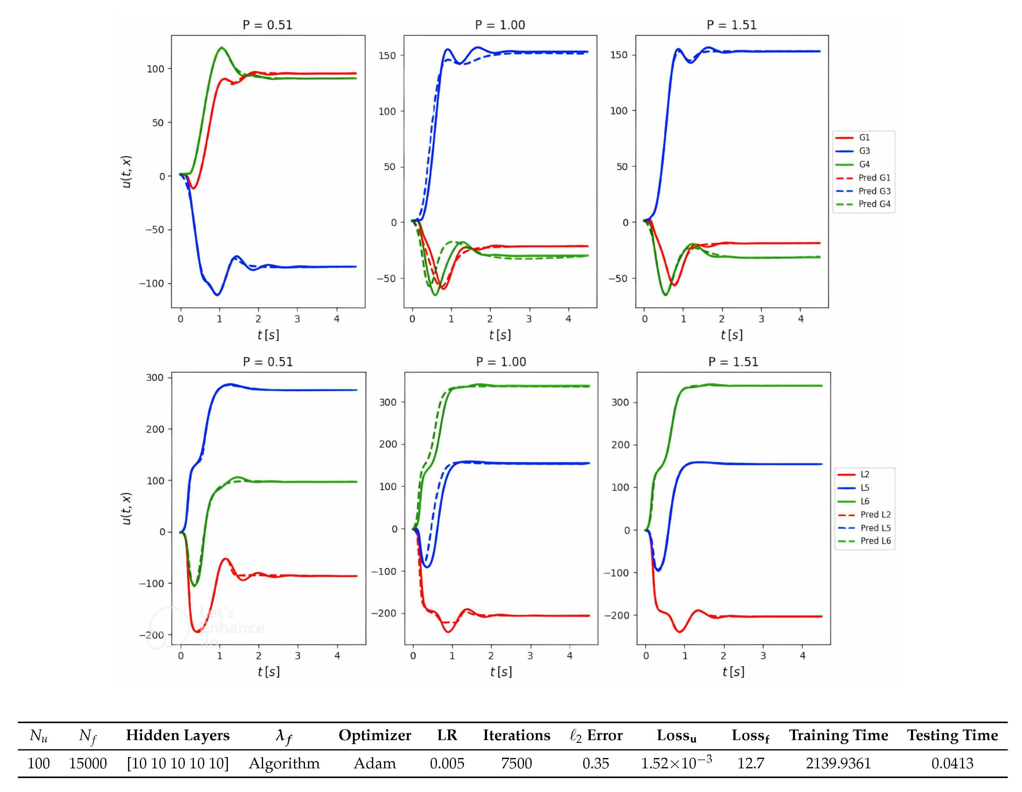
Figure 11 displays the analysis of the six-bus power system, employing a PINN. Given its increased complexity, certain hyperparameters were adjusted, e.g., the number of iterations was increased to ensure the effective training of this system.

For solving the differential equations, the average computational time of ode45 was 1.371 s, while the PINN took over 0.0185 s. This represents an increase of almost 35 times compared to the speed of ode45. Moreover, to ensure optimal performance, the ${\lambda }_f$ value needed to be adjusted from 1 to 0.001 starting from iteration 100 as in the previous case. Given the wider range of angle changes in this case, the impact of loss weights became even more significant. It may be possible to reduce the number of $N_u$ or $N_f$ at the expense of slightly reduced accuracy. However, in this particular case, the difference in accuracy was almost negligible.

A favorable case for the last system studied, i.e., the 14-bus power system, is depicted in Figure 12. Despite the heightened complexity, it is notable that the training and testing speed remained similar to the previous case, as did the ${\mathsf{\ell }}_2$ error. To appropriately adjust the loss weights, the value of ${\lambda }_f$ was decreased to 0.0001. In addition, different ranges of $N_u$ and $N_f$ points were explored. Increasing the number of $N_u$ points proved beneficial for accuracy at the initial condition points; however, it sometimes affected the accuracy of the remaining points. Therefore, in each specific case, tuning these points becomes crucial in order to achieve the best accuracy while considering the trade-offs within the problem.

The speed of the PINN also increased significantly to 0.1133 s, compared to 4.7291 s for ode45, making it roughly 42-times faster.

Errors in PINNs can stem from various factors: (1) Model Complexity and Architecture—errors can occur if the neural network’s architecture is too simplistic to effectively model the underlying physical processes; on the flip side, overly complex models may overfit, struggling to generalize to new conditions and leading to inaccuracies when applied to scenarios not encountered during training. (2) Quality and Quantity of Data—despite PINNs needing less data than traditional neural networks, the data’s quality, particularly the initial and boundary conditions, is vital; data that are lacking or contain noise can hinder the learning process of the network. (3) Loss Function and Regularization—the error can also be influenced by the chosen loss function and how its various components (like data loss and physics-informed loss) are balanced; an imbalance can cause the network to disproportionately focus on one aspect, leading to inaccuracies. (4) Numerical Stability and Optimization—the optimization process itself can be a source of error; issues like local minima, slow convergence, or numerical instabilities can affect the model’s accuracy. Additionally, the choice of optimizer and the learning rate setting are crucial in determining the network’s performance.

Observations from the one-bus system, three-bus system, and six-bus system showed the convergence of angles under various p values, indicating stability across multiple scenarios in these systems. Conversely, the 14-bus system displayed instances of non-convergence, particularly in curves like G3 and L10, when the p values were set at 0.51, 1.27, and 1.51. This indicates that PINNs can capture accurate physical phenomena and inform us about stable or unstable systems. Analyzing Figure 10, Figure 11 and Figure 12, it is evident that the predictions made by physics-informed Neural Networks (PINNs) across all systems closely aligned with the ground truths, which are depicted using results from ode45. This alignment underscores PINNs’ proficiency in accurately handling each system. Interestingly, the highest accuracy was observed in the 14-bus system, followed by the 3-bus system, and then the 6-bus system. This pattern indicates that the accuracy of PINNs may not be directly related to the size of the system but rather influenced by other factors. This observation reinforces the notion that PINNs adeptly maintain accuracy while scaling up in size. Therefore, engineers can use PINNs for various system sizes. Figure 13 presents the training and testing times on a logarithmic scale, further highlighting the superior efficiency of PINNs compared to ode45. Notably, PINNs exhibited an increasing speed advantage over ode45 as the system size expanded. This efficiency stems from PINNs’ unique approach of direct function mapping, which enables significantly faster inference than traditional methods.

Lastly, the careful exploration of the learning rate and hidden layer size was also conducted. The best results were achieved with the values presented in the tables, leading to the decision to maintain these parameter settings. Similarly, a deliberate choice was made to use the same optimizer across all cases, ensuring consistency in the experimental setup.

5.5. Ablation Study of PINNs in Power Systems

Based on the empirical findings presented in the preceding sections, several significant observations can be derived. Firstly, certain parameters exhibit stability and remain relatively unchanged regardless of the system’s scalability. These parameters can include the neural network’s size and depth, the choice of the optimizer, and its corresponding learning rate. Conversely, the remaining parameters require adjustments depending on the system’s scalability.

The optimal number of iterations seems more dependent on the complexity of the angle curves rather than the system’s dimensions. Consequently, it is advisable to establish the maximum iteration value based on a tolerance threshold, rather than relying on a fixed numerical quantity. In the preceding subsection, it was observed that the LBFGS optimizer lacks the ability to set a specific maximum number of iterations. Instead, the maximum training time is contingent upon either the maximum number of evaluations or a specified tolerance level. Nevertheless, in the case of using other optimizers, our experimental investigations consistently revealed that a maximum of 10,000 iterations proved adequate for all tested scenarios.

The adjustment of $N_u$, $N_f$, and ${\lambda }_f$ presents the main challenge. In order to compare how changes in these parameters may impact the neural network’s performance, we modified the employed optimizer to Adam with a fixed learning rate of $5\times {10}^{-3}$ and incorporated the gradient-based algorithm from (9). By adopting this approach, we effectively overcame the challenge of manually selecting the loss weight ${\lambda }_f$, as it was now determined by the algorithm. Moreover, we could now set the value of the maximum number of iterations to a fixed number depending on the system and $N_f$ to 15,000 and then proceed to fine-tune $N_u$. This enabled us to observe and understand how variations in the parameter $N_u$ impacted the L2 error of the neural network.

Figure 14 illustrates the impact of varying the number of $N_u$ points on the accuracy of the PINN model for power systems with different numbers of buses. Surprisingly, unusual behavior was observed, attributed to the imbalance of the $N_f$ hyperparameter in the neural network’s loss function. Intuitively, one might expect that increasing the number of $N_u$ data points would lead to a reduction in the normalized error. However, based on the results, there appeared to be minimal difference in the selection of this hyperparameter.

Figure 15 displays the results obtained from employing the gradient-based update algorithm that adjusted both losses for the six-bus system. Observing the graph, we notice that the training time increased, while the testing time remained relatively stable. Moreover, there was a decrease in the L2 error, indicating a positive effect from the algorithm’s use in terms of accuracy. Similar behavior could be expanded to the rest of the bus power systems.

As mentioned earlier in this section, altering the number of neurons did not appear to adversely affect the experiments either. Figure 16 demonstrates this relationship for the last two cases. Intuitively, increasing the number of neurons had the potential to decrease the $L_u$ loss, but it could also result in an increase in the $L_f$ loss. As a result, the overall loss behavior did not follow a specific pattern and could vary depending on the specific case and configuration.

Lastly, to ensure accuracy across the entire domain $\mathrm{\Omega }$, the proper adjustment of both $N_u$ and $N_f$ is also crucial. Increasing $N_u$ can improve the accuracy of initial condition points, but it is equally important to increase $N_f$ in tandem. From the experimental results, a recommended guideline is to maintain at least a 30-fold difference between the numbers of $N_f$ and $N_u$. This balanced proportion contributes to better accuracy. Moreover, to further enhance accuracy, it is advantageous to increase both $N_u$ and $N_f$ while maintaining their proportional difference. However, this approach comes with the trade-off of significantly increased the training time and the number of iterations required.

It is important to note that PINN-based methods are fundamentally distinct from traditional approaches. The key difference lies in their direct function mapping, which allows for exceptionally rapid inference. Given this unique characteristic, there are currently no existing methods that can match PINNs in terms of inference speed. Moreover, the primary focus of our work was a comprehensive in-depth analysis of PINNs, specifically in the context of power system transient stability across various levels of grid complexity. This specialized focus on PINNs and their unique advantages in inference speed made a direct comparison with other methods less relevant to the goals and scope of our research.

6. Conclusions

Our study breaks new ground in evaluating physics-informed Neural Networks (PINNs) for power system transient stability across various grid complexities. It is the first to investigate PINNs in a range of power system scales, demonstrating their ability to maintain accuracy even as complexity increases. This finding is crucial, proving the robustness of PINNs in diverse settings. Another notable contribution of our research is the development of a novel method for adjusting loss weights, significantly improving PINNs’ adaptability to different power system models and enhancing PINNs’ flexibility and effectiveness in different system setups. Overall, our findings position PINNs as a potent tool in power system analysis, effectively merging data-driven approaches with core physical principles. This study not only enhances the understanding of PINNs’ performance in complex scenarios but also opens new avenues for their application in real-world power system challenges. Future research could explore PINNs in more complex systems and real-time applications, further optimizing their performance in power system stability and dynamics. Additionally, future directions could include maintaining the key physical properties and structures of systems [17,40] and providing theoretical guarantees for these methods.