Systematic Review

Artificial Intelligence-Based Algorithms in Medical Image Scan Segmentation and Intelligent Visual Content Generation—A Concise Overview

by
Zofia Rudnicka
,
Janusz Szczepanski
and
Agnieszka Pregowska
*
Institute of Fundamental Technological Research, Polish Academy of Sciences, Pawinskiego 5B, 02-106 Warsaw, Poland
*
Author to whom correspondence should be addressed.
Electronics 2024, 13(4), 746; https://doi.org/10.3390/electronics13040746
Submission received: 8 January 2024 / Revised: 7 February 2024 / Accepted: 8 February 2024 / Published: 13 February 2024

Abstract

:
Recently, artificial intelligence (AI)-based algorithms have revolutionized the medical image segmentation processes. Thus, the precise segmentation of organs and their lesions may contribute to an efficient diagnostics process and a more effective selection of targeted therapies, as well as increasing the effectiveness of the training process. In this context, AI may contribute to the automatization of the image scan segmentation process and increase the quality of the resulting 3D objects, which may lead to the generation of more realistic virtual objects. In this paper, we focus on the AI-based solutions applied in medical image scan segmentation and intelligent visual content generation, i.e., computer-generated three-dimensional (3D) images in the context of extended reality (XR). We consider different types of neural networks used with a special emphasis on the learning rules applied, taking into account algorithm accuracy and performance, as well as open data availability. This paper attempts to summarize the current development of AI-based segmentation methods in medical imaging and intelligent visual content generation that are applied in XR. It concludes with possible developments and open challenges in AI applications in extended reality-based solutions. Finally, future lines of research and development directions of artificial intelligence applications, both in medical image segmentation and extended reality-based medical solutions, are discussed.

1. Introduction

The human brain, a paramount example of evolutionary biological sophistication, transcends its anatomical categorization. Constituted by an estimated 86 billion neurons linked through an intricate web of synapses (ranging in the trillions), it is the epicenter of our cognitive, emotional, and consciousness-related functions [1]. This masterful structure of the central nervous system represents a nexus of myriad neurobiological processes, intricately overseeing sensory input conversion, motor responses, and advanced cognitive functionalities. As a product of relentless evolutionary adaptations spanning millions of years, the brain epitomizes the apex of neurobiological optimization, synergizing complex neural circuitry with higher-order cognitive undertakings such as cognitive reasoning, emotional homeostasis, and the intricate processes of memory encoding, storage, and retrieval [1,2,3]. Thus, the human brain is a super-complex system whose functioning and intelligence depend rather on the type of neurons (depending on their role in the brain), their connections, and the way of supplying energy to neurons than the number of neurons [2]. It is an ideal reference model for the foundations of Artificial Intelligence (AI) [3,4]. Despite many advances, we are unsure of human brain complexity. Thus, the study of the foundations of natural intelligence may contribute to both the understanding of the general mechanics of intelligence regarding pervasive brain-inspired systems [5,6], and the formulation of intelligent entities. At the moment, artificial intelligence is far from replicating the entire human brain. Certain aspects of neural networks and cognitive functions have played a key role in developing AI models. First, the structure of the neural network reflects the interconnections of neurons in the brain. Consequently, the AI-based model can process information in a hierarchical and interconnected way (pattern recognition and decision-making). Also, the process of training neural networks itself is inspired by the adaptive nature of human cognition. With the development of AI, including deep learning, algorithms are becoming more precise, faster, and able to faithfully reproduce the processes taking place in the human brain. Indeed, AI is thus rapidly permeating virtually all aspects of everyday life. However, it may also be responsible for the introduction of errors in decision-making processes such as those related to bias in algorithms, deriving in particular from disproportionate and overrepresentation of certain data in electronic databases. A ready-made dataset may include built-in biases or biases introduced by the data scientist in the prefiltering step [7]. In turn, storing information and recalling information in networks is based on the model of human memory [8]. Another important aspect of AI-based models is their computational efficiency. The human brain can perform multiple tasks simultaneously, which has led to parallel processing architectures in AI systems to reduce the amount of resources needed for computation [9]. However, all of the above aspects of artificial intelligence are still at an early stage of development and require improvement.
Thus, processing and analysis of biomedical data for diagnostic purposes is a multidisciplinary field that combines AI, machine learning (ML), biostatistics, and time series analysis, as well as statistical physics and algebra (e.g., graph theory) [3]. Variables derived from biomedical phenomena can be described in several ways and in different domains (time, frequency, spectral values, spaces of states describing the biological system), depending on the characteristics and type of signal. Effective diagnosis of the early stages of the disease, as well as the determination of disease development trends, is a very difficult issue that requires taking into account many factors and parameters. Therefore, the state spaces of biomedical signals are huge and impossible to fully search, analyze, and classify even with the use of powerful computational resources. Therefore, it is necessary to use artificial intelligence, in particular bio-inspired AI methods, to limit research to a smaller but significant part of the state space.
Recently, computer-generated three-dimensional (3D) images have become increasingly important in medical diagnostics [10,11]. The applications of 3D imaging in medical diagnostics enable increased spatial awareness of users. Traditional images can flatten or distort anatomical features, which can make accurate assessment of relationships between structures much more difficult, thus making an accurate diagnosis. For example, it allows one to plan the course of surgery based on 3D reconstruction of the patient’s body or its parts. Such preoperative knowledge can significantly improve the precision and success of surgery, reducing the risk of complications. Additionally, 3D imaging of complex diseases and pathologies allows for better visualization of complex structures. It can also have an educational function for both students and patients. In particular, the so-called extended reality (XR) Metaverse is increasingly used in health care and medical education, while it enables a deeper experience of the virtual world, especially through the development of depth perception, including the rendering of several modalities like vision, touch, and hearing [12]. In fact, medical images have different modalities, and their accurate classification at the pixel level enables the accurate identification of disorders and abnormalities [13,14]. However, creating a 3D model of organs and/or their abnormalities is time-consuming and is often done manually or semiautomatically [15]. AI can automate this process and also contribute to increasing the quality of the resulting 3D objects [16,17] as well as visual content in the metaverse [4,18]. To give the users a real sense of visual immersion, the developers should implement virtual objects of high quality [19]. In the context of medicine, it is combined with good-quality medical data and their classification/segmentation algorithms with high accuracy to faithfully reproduce the content in virtual three dimensions.
In this study, we aim to determine existing research gaps in the area of broadly understood medicine, including clinical trials in the application of explainable artificial intelligence. For that reason, this paper focuses on an overview of artificial intelligence-based algorithms in medical image scan segmentation and intelligent visual content generation in extended reality, including different types of neural networks used and learning rules, taking into account mathematical/theoretical foundations, algorithm accuracy, and performance, as well as open data availability. Specifically, we aim to answer the following research questions. Can AI-based algorithms be used for the accurate segmentation of medical data? How can AI-based algorithms be beneficial in extended reality-based technologies?

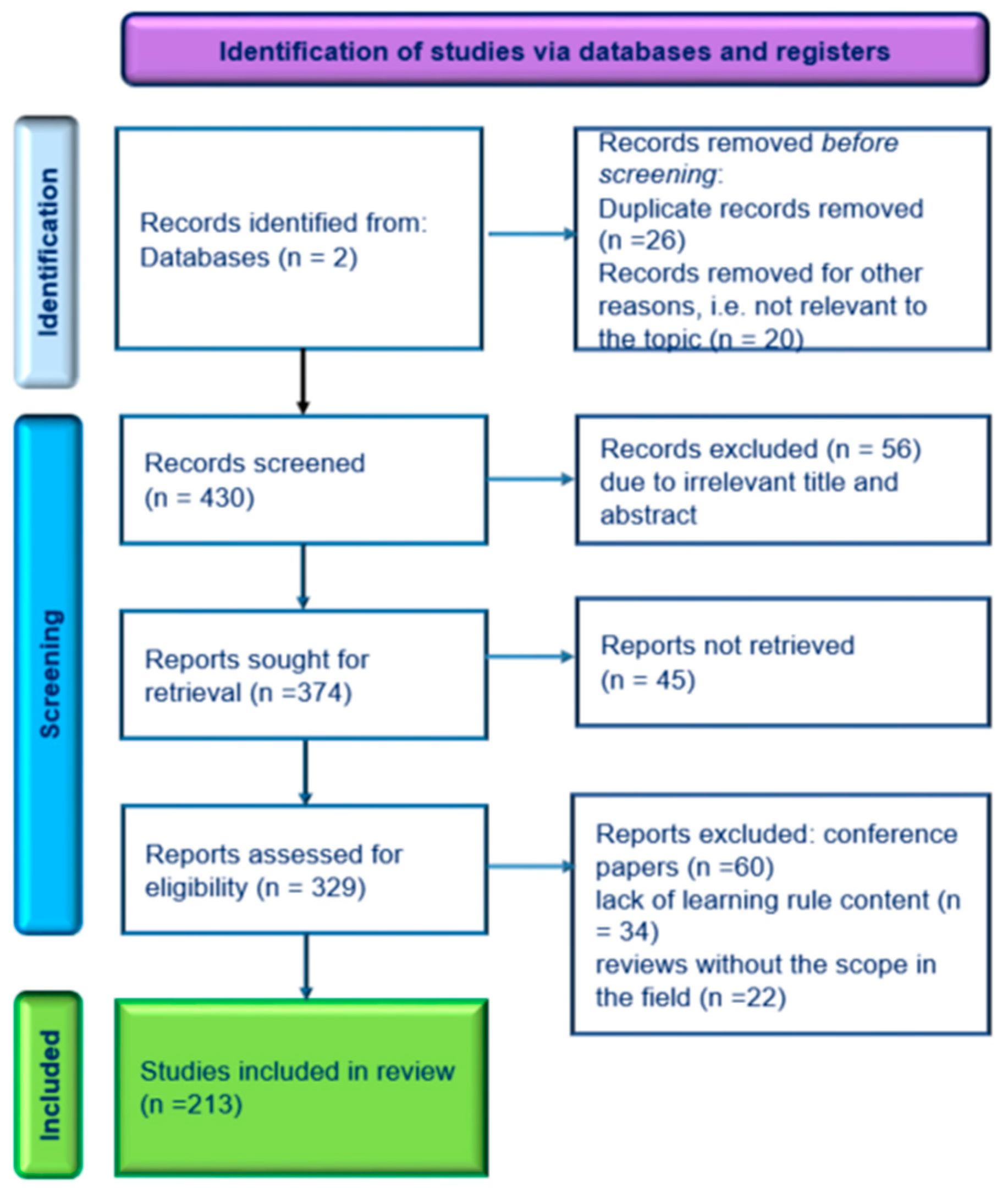
2. Materials and Methods

The methodology of the systematic review was based on the PRISMA statement, which was published in several journals [20], and its extension—PRISMA-S [21]. We considered recent publications, reports, protocols, and review papers from Scopus and Web of Science databases. The keywords were artificial intelligence, machine learning, extended reality, mixed reality (MR), virtual reality (VR), metaverse, learning algorithms, learning rules, signal classification, signal segmentation, medical image scan segmentation, segmentation algorithms, classification algorithms, and their variations. The selected sources were analyzed in terms of compliance with the analyzed topic, and then their contribution to medical image scan segmentation. First, the obtained title and abstract were independently evaluated by the authors. The duplicated records have been removed. Moreover, we have considered the inclusion of criteria-like publications in the form of journal papers, books, and proceedings, as well as technical reports. The search was limited to full-text articles in English, including electronic publications before printing. Also, exclusion criteria like PhD theses and materials not related to medical image scan segmentation and artificial intelligence-based algorithms have been adopted. Subsequently, articles meeting the criteria were retrieved and analyzed. The documents used in this study were selected based on the procedure presented in Figure 1. In the first step, duplicate records and resources not relevant to the topic of the conducted study have been removed. Next, the resources whose titles and abstracts were not relevant to the topic have been excluded. Then, the resources that were not retrieved were removed from the study. In the end, conference papers, reviews of predominant areas outside the study topic, and sources that do not contain information about the learning algorithms used have been excluded. Finally, 213 documents were taken into account. The current study has the following limitations: (1) the exclusion of resources without information concerning critical information like neural networks, neuron models, information details in datasets, input, and output parameters, and learning rules; (2) the sources included were designed mainly retrospectively, and most of the research is laboratory-based in nature and has not entered clinical practice; (3) the study takes into account Scopus and Web of Science databases (however, this ensures the integrity of the dataset); and (4) potential language bias (i.e., conducted of comprehensive search, only English-language resources).
In this study, we concentrate on the theoretical foundation of neural communication, the model of neurons, the type of neural networks, and learning rules, with a special emphasis on their application in medical image scan segmentation and intelligent visual content generation. We analyzed artificial neural networks (ANNs), convolutional neural networks (CNNs), recurrent neural networks (RNNs), spiking neural networks (SNNs), generative adversarial networks (GANs), graph neural networks (GNNs), and “transformers.” The first one is the simplest neuron model (i.e., perceptions) and can process the information only in one direction. The second one consists of multilayer perceptrons and contains one or more convolutional layers that are responsible for the creation of feature maps, which are subjected to nonlinear processing. RNNs save the output to the processing nodes and feed the result back into the network (bidirectional information processing). The last type is closest to the real nervous system. SNNs transmit the information when the membrane potential of a neuron does not reach the threshold in every cycle of propagation like other listed neural networks. Another field that we analyzed in the context of medicine is learning rules, including backpropagation (i.e., in which the weight of the network is calculated according to the chain rule of the partial derivatives of the error function), ANN–SNN conversion (i.e., transforming SNNs into ANNs and application of the learning rules that are efficient in ANNs), supervised Hebbian learning (i.e., the postulate based on the rule that when the human brain is learning, the neurons activate), reinforcement learning with supervised models (i.e., it enables monitoring of the reaction on the learning rule), the chronotron (i.e., learning rules that take into account both spiking neuron and the time of spiking), and biologically inspired network learning algorithms.

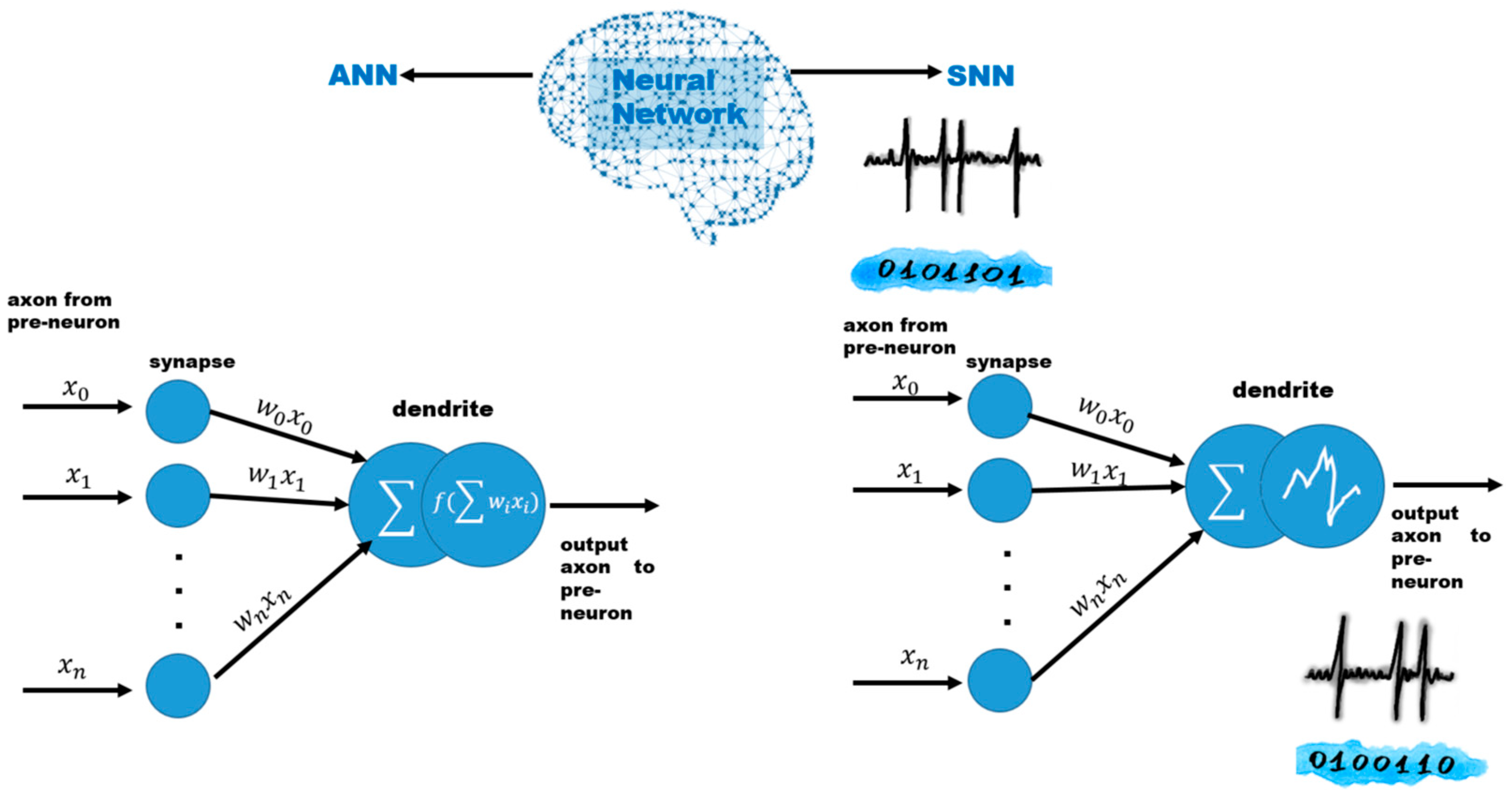
3. Neural Communication

Neurons, which are basic brain building blocks, function as the core computational units of the brain, underpinning the vast expanse of conscious and subconscious processes, and defining our neural identity with each electrochemical interaction [16]. Neurons communicate with other neurons and non-neuronal cells like muscles and glands by biological connections called “chemical synapses”, which are the communication points, by which sending nerve cells called presynaptic neurons transmit the message to receiving nerve cells called the postsynaptic neurons. The presynaptic neurons release neurotransmitters, a diverse group of chemicals, into the synaptic cleft (i.e., the small gap at which neurons communicate). Following the release, these compounds traverse the synaptic gap, interact with receptors on the postsynaptic membrane, and elicit a series of intracellular events, potentially leading to the generation of an action potential, a transient depolarizing event propagated along the neuronal membrane.
Since the famous experiments of Adrian [22,23,24], it is assumed that in the nervous systems (including the brain), information is transmitted through weak electric currents (in the order of 100 mV), in particular employing action potentials (spikes) that are a transient, sudden (1–2 millisecond) change in the membrane potential of the cell/neuron associated with the transmission of information [25]. The stimulus for the creation of an action potential is a change in the electric potential in the cell’s external environment. A wandering action potential is called a nerve impulse. In the literature [26,27], it is assumed that the sequences of such action potentials, called spike trains, play a key role in the transmission of information, and the times of appearance of these action potentials play a significant role. Mathematically, such time sequences can be and are modeled in particular after digitalization as trajectories (or their variants) of certain stochastic processes (Bernoulli, Markov, Poisson, …) [26,27,28,29,30,31,32,33].

4. Taxonomy of Neural Network Applied in the Medical Image Segmentation Process

The artificial neural networks (ANNs) are constructed with the perceptron neuron model [34] that is based on the binary decision rule. If the linear weights w i of the sum of the input signals (input vector x i ) exceed the threshold t h r , the neuron fires (i.e., the output is equal to 1) or if not, the output is equal to 0.
The basic input function is described as follows
f x = 1 ,   i f   w 1 x 1 + w 2 x 2 + + w n x n t h r 0 ,   o t h e r w i s e
The output vector of all neurons in the l -th layer can be expressed, as well as the combination of the linear transformation and nonlinear mapping (i.e., ANN activation values) [29]:
a l = h W l a l 1 ,   i = 1 , , M
where W l is the weight matrix between layer l and l 1 , and h ( · ) denotes the activation function, in this case, the rectified linear unit (ReLU) h x = x + = max 0 , x and the vector a l denotes the output of all neurons in the l -th layer. Formula (2) has been quoted following the designations in [35]. Neuron models from the integrate-and-fire family are among the simplest; however, they are also the most frequently used. They are classified as spiking models. From a biophysical point of view, action potentials are the result of currents flowing through ion channels in the membrane of nerve cells. The integrate-and-fire neuron model [36,37] focuses on the dynamics of these currents and the resulting changes in membrane potential. Therefore, despite numerous simplifications, these models can capture the essence of neuronal behavior in terms of dynamic systems.
The concept of integrate-and-fire neurons is the following. The input ion stream depolarizes the neuron’s cell membrane, increasing its electrical potential. An increase in potential above a certain threshold value   U t h r produces an action potential (i.e., an impulse in the form of Dirac’s delta), and then the membrane potential is reset to the resting level. The leaky integrate-and-fire (LIF) neuron model [36,37] is an extended model of the integrate-and-fire neuron, in which the issue of time-independent memory is solved by equipping the cell membrane with a so-called leak. This mechanism causes ions to diffuse in the direction of lowering the potential to the resting level or another level U 0 U l e a k < U t h r . Thus, the third generation of neural networks, i.e., the spiking neural networks (SNNs) [38], are mostly based on the LIF, where the membrane potential U ( t ) is determined by the equation
τ m d U d t = [ U t U r e s t ] + R m I t  
where τm is the membrane time constant of the neuron, Rm is total membrane resistance, and I(t) is the electric current passing through the electrode. The spiking events are not explicitly modeled in the LIF model. Instead, when the membrane potential U(t) reaches a certain threshold Uth (spiking threshold), it is instantaneously reset to a lower value Urest (reset potential) and the leaky integration process starts a new one with the initial value Ur. To mention just a little bit of realism regarding the dynamics of the LIF model, it is possible to add an absolute refractory period Δabsimmediately after U(t) hits Uth. During the absolute refractory period, U(t) might be clamped to Ur, and the leaky integration process is reinitiated following a delay of Δabs after the spike. More generally, the membrane potential (3) can be presented as
U t = i = 1 N ω i t i < t u ( t t i )
where u ( t ) is a fixed causal temporal kernel that is an operation that allows scale covariance and scale invariance in a causal–temporal and recursive system over time [39] and ω i ,   i = 1 , ,   N denotes the strength of neuron synapses. Following Equation (2), the neuron’s output m l ( t ) (membrane potential after the neuron firing) can be described as follows [29]
m l ( t ) = v l ( t 1 ) + W l x l 1 ( t )   l = 1 , , N
where v l denotes the membrane potential before the neuron fires, W l is the weight in the l -th layer ( l denoted layer index), and x l 1 ( t ) is the input from the last layer. Thus, to avoid the loss of information, the “reset-by-subtraction” mechanism was introduced [40]
v l t v l t 1 = W l x l 1 ( t ) ( H ( m l t θ l ) θ l )
where v l t is membrane potential after firing, m l t —membrane potential before firing, H ( m l t θ l ) refers to the output spikes of all neurons, and θ l is a vector of the firing threshold θ l . There are also some applications of the concepts of the meta-neuron model in SNNs [41]. The main differences between the LIF neuron and meta-neurons stay in the integration process, where meta-neurons use a second-order ordinary differential equation and an additional hidden variable. The basic differences between ANNs and SNNs (taking into account the type of neuron models) are presented in Figure 2. Thus, the crucial difference between ANNs and SNNs is the fact that ANNs use continuous activation functions and represent information with continuous values, while SNNs use a spiking model, conveying information through discrete spikes in time.

4.1. Convolutional Neural Network

The most commonly used deep neural network (DNN) in medical image classification is the two-dimensional (2D) convolutional neural network (CNN) [42,43]. In Figure 3, the basic scheme of the CNN is presented. It consists of three layers: input, output, and hidden. The principle of CNN operation is based on linear algebra, in particular matrix multiplication. CNNs consist of three types of layers: a convolutional layer, a pooling layer, and a fully connected layer. In fact, most computations are performed in the convolutional layer or layers. The image (pixels) is converted into binary values and patterns are searched. Every convolutional layer operates a dot product between two matrices, i.e., one matrix is a set of learnable parameters (kernel), and the second matrix is a limited part of the receptive field. Each subsequent layer contains a filter/kernel that allows one to classify features with greater efficiency. A pooling layer reduces the number of parameters in the input, which causes the loss of part of the information calculated in the common layer/layers; however, it allows for improvement in the efficiency of the CNN network. This operation is performed by sliding windows [44]. Next, the output of these two layers is transformed into a one-dimensional vector, i.e., input to the fully connected layer. In this last type of layer, image classification based on the features extracted in the previous layers is performed, i.e., the object in the image is recognized. The output y i , j ( k ) from CNNs can be described as follows
y i , j ( k ) = σ ( l = 1 L m = 1 M x i + l 1 , j + m 1 l w l . m k + b ( k ) )
where x i , j l denotes input to the network at the spatial location ( i , j ) , σ is the activation function, w l . m k is the weight of the m th kernel at the l th channel producing the k th feature map, and b ( k ) is the bias for the k th feature map.
In the case of large datasets, CNN achieves high efficiency and is resistant to noise [45]. The crucial disadvantages of CNNs in image processing are high computational requirements and difficulties in achieving high efficiency in the case of small datasets (i.e., if the dataset is too small, the network may overfit to training data and poorly recognize new data).

4.2. Recurrent Neural Network

Another neural network commonly applied in medical data analysis is the recurrent neural network [46]. In Figure 4, the basic scheme of the RNN is presented. This type of network contains at least one feedback connection. The network presented in Figure 3 consists of three layers—input, output, and hidden—as well as a feedback connection. The output of RNN can be expressed as [47]
y i = W h y   H W h h h i 1 + W x h x i + b h h i + b y
where x i , i = 1 , , T is the input sequence of T states ( x i ,   ,   x T ) with x i R d ,   W x h   , W h y   , W h h   denotes weight matrices,   b h , b y are bias vectors, and H is the nonlinear activation function, for example, ReLU, sigmoid f x = 1 1 + e x , Tanh function (hyperbolic tangent) f x = e x e x e x + e x . The network operation is recursive since the hidden layer state depends on the current input and the previous state of the network. Thus, the hidden state h i 1 is the memory of past inputs.
Thus, the RNN can operate on the sequential dataset and has an internal memory. It may have many inputs. However, RNNs exhibit learning-related problems, namely, vanishing gradients (i.e., in the case of small gradients, the updates of parameters are irrelevant) or exploding gradients (i.e., superposition of large error gradients leading to large parameter updates). These contribute to the long training process, low level of accuracy, and low network performance.

4.3. Spiking Neural Networks

Besides the artificial neural networks, i.e., CNNs, and RNNs, one can also be applied to the medical signals’ bio-inspired neural networks, such as spiking neural networks [47,48]. In Figure 5, the basic scheme of the SNN is presented. It consists of three layers: input, output, and hidden. SNNs encode information taking into account spike signals, and shells are promising in effectuating more complicated tasks, while more spatiotemporal information is encoded with spike patterns [49]. They are mostly based on the LIF neuron model. SNNs were formulated to map organic neurons, i.e., the appearance of the presynaptic spike at synapse triggers the input signal i ( t ) (the value of the current) that in simplified cases can be written as follows
i t = 0 S j s t exp ( s τ s ) d s
where τ s denotes synaptic time constant, S j is a presynaptic spike train, and t is time [50]. In contrast, the majority of DNNs do not take into account temporal dynamics [51]. In fact, SNNs show promising capability in playing a similar role as living brains. Moreover, the binary activation in SNNs enables the development of dedicated hardware for neuromorphic computing [52]. The potential benefits are low energy usage and greater parallelizability due to the local interactions.

5. Learning Algorithms

The heart of artificial intelligence is its learning algorithms. At their core, they strive to automate the learning process, enabling machines to recognize patterns, make decisions, and predict outcomes based on data. Their design is often a balance between theoretical rigor and practical applicability. While mathematics and statistics provide the foundation, translating these into algorithms that can operate on vast and diverse datasets requires creative programming skills [28]. One can distinguish many types of network training algorithms [53]. Below, we briefly discuss the most important of them, taking into account the theoretical foundations.

5.1. Backpropagation Algorithm

The most commonly used learning algorithm is the backpropagation (BP) algorithm. It overweights optimizations via error propagation in the neural networks. BP plays a pivotal role in enabling neural networks to recognize complex and nonlinear patterns from large datasets [29,54,55]. From the mathematical point of view, it is a calculation of the cost function, which minimizes the calculated error of the output using gradient descent or the delta rule [56]. It can be split into three stages: forward calculation, backward calculation, and computing the updated biases and weights. The input to the hidden layer H j is the weighted sum of the outputs of the input neurons and can be described as [57]
H j = b i n + i = 1 n x i w i j
where x i is the input to the network (input layer), n is the number of neurons in the input layer, b i n is the bias input layer, and w i j denotes the weight associated with the i -th input neuron and the j -th hidden neuron. The output y k is as follows
y k = b h + j = 1 m w j k F ( H ( j ) )
where F ( H ( j ) ) is a transfer function, k is the number of neurons in the hidden layer, and b h is the bias of the hidden layer. The most commonly used transfer function is the sigmoid transfer function F H j = 1 1 + e ( H j ) . The backpropagation algorithm is especially effective when used in multilayered neural architectures such as feed-forward neural networks, convolutional neural networks, and recurrent neural networks [32]. In image recognition, CNNs, energized by BP, can independently identify hierarchical features, from basic edges to detailed structures. Similarly, RNNs, amplified by BP, are adept at sequence-driven tasks like machine translation or speech recognition, as they incorporate previous data to influence present outputs. It is one of the most effective deep learning methods. However, BP requires large amounts of data and enormous computational resources.

5.2. ANN–SNN Conversion

Artificial neural networks and spiking neural networks are both computational models inspired by biological neural networks. While ANNs have been the mainstream for most deep learning applications due to their simplicity and effectiveness, SNNs are gaining traction because they mimic the behavior of real neurons more closely by using spikes or binary events for communication. To obtain similar accuracy for the SNN-based algorithm as the algorithm using ANN, for example, the BP-type training rule consumes a lot of hardware resources. The already existing platforms have limited optimization possibilities. Thus, the conversion of ANNs to SNNs seeks to harness the energy efficiency and bio-realism of SNNs without reinventing the training methodologies [34], while it is based on the ReLU activation function and LIF neuron model [58]. The basic principle of the conversion of ANNs to SNNs is mapping the activation value of the ANN neuron to the average postsynaptic potential (in fact, firing rate) of SNN neurons, and the change in membrane potential (i.e., the basic function of spiking neurons) can be expressed by the combination of Equations (2) and (6) [35]
v l t v l t 1 = W l x l 1 ( t ) s l t θ l
Here, s l t refers to the output spikes of all neurons in layer l at time t .
Tuning the right thresholds is paramount for the SNN to effectively and accurately represent information. Incorrectly set thresholds could lead to spiking that is either too frequent or too rare, potentially affecting the accuracy of the SNN post-conversion [41]. On the other hand, the neuromorphic hardware platforms that support SNNs natively can primarily offer energy efficiency benefits by converting ANNs to SNNs. Due to their event-driven nature, SNNs can be more computationally efficient [42]. However, the challenge lies in maintaining accuracy post-conversion. Some information might be lost during the transition, and not all ANN architectures and layers neatly convert to their SNN equivalents. The conversion from ANNs to SNNs is a promising direction, merging the advanced training methodologies of ANNs with the energy efficiency of SNNs. As we delve deeper into the realm of neuromorphic computing, this conversion process will play a pivotal role in bridging traditional deep learning with biologically inspired neural models [43,44].

5.3. Supervised Hebbian Learning (SHL)

Taking into account artificial intelligence, supervised Hebbian learning (SHL) can be described as a general methodology for weight changes [58]. Thus, this weight increases when two neurons fire at the same time, while it decreases when two neurons fire independently. According to this rule, the change in weight can be written as
w = η ( t o u t t d )
where η is the learning rate (in fact, the small scalar that may vary with time, η > 0 ), t o u t the actual time of the postsynaptic spike, while t d is the time of firing of the second presynaptic spike [59,60]. The crucial disadvantage of Hebbian learning is the fact that when the number of hidden layers increases, the efficiency decreases, while in the case of four layers, it is still competitive [52].

5.4. Reinforcement Learning with Supervised Models

According to the additional constraints in the SHL rule, reinforcement learning with supervised models (ReSuMe) was proposed [60]. ReSuMe is a dynamic hybrid learning paradigm. It effectively combines the resilience of reinforcement learning (RL) with the precision of supervised learning (SL). This fusion empowers ReSuMe to leverage feedback-driven mechanisms inherent in RL and take advantage of labeled guidance typical of SL [43,44,45]. The difference with SHL is that the learning signal is expected not to have or have a marginal direct effect on the value of the postsynaptic somatic membrane potential [61,62,63], and thus the synaptic weights are modified as follows
d d t w j i t = a [ S d t S j t ] S ¯ i t
where a denotes learning rate, S d is desired/targeted spike train, S j t is the output of the network (spike train), and S ¯ i t expresses the low-pass filtered input spike train. ReSuMe guides one of its most salient features of exploration. By leveraging labeled data via SL, ReSuMe can effectively steer RL exploration, ensuring agents avoid falling into the trap of suboptimal policies. The hybrid nature of ReSuMe also grants it a unique resilience, especially in the face of noisy data or in reward-scarce environments. Moreover, its adaptability is noteworthy, making it an ideal choice for tasks that combine immediate feedback (through SL) with long-term strategic maneuvers (through RL). However, like all things, ReSuMe is not without challenges. A potential bottleneck in ReSuMe is computational complexity, as managing both RL and SL can sometimes strain computational resources. Another challenge is the precise tuning of the a coefficient. The key is to find a balance where neither RL nor SL overly dominates the learning process. By melding immediate feedback from supervised learning with a deep reinforcement learning strategy, ReSuMe establishes itself as a formidable tool in machine learning [55,56,58].

5.5. Chronotron

The chronotron, by its essence, challenges and reshapes our understanding of how information can be encoded and processed in neural structures [56,61]. Traditional neural models have predominantly focused on the spatial domain, emphasizing the architecture and interconnections between neurons. While this spatial component is undeniably critical, it offers only a part of the full informational symphony that the brain plays. Just as the rhythm and cadence of a song contribute as much to its essence as its melody, in the vast theater of the brain, timing is not just a factor; it is a storyteller in its own right. The brilliance of the chronotron lies in its ability to discern and respond to this temporal narrative. Unlike its counterparts, which often treat time as a secondary parameter, the chronotron places it center stage. As a consequence, it acknowledges and leverages the intricate interplay of spatial and temporal dynamics in neural computation. This means that it not only considers which neurons are firing but also pays meticulous attention to when they fire relating to one another. Thus, the membrane potential is
u t = η t + j w j t j f t ε j ( t , t j f )
where the η model’s refractoriness is caused by the past presynaptic spikes, w j is the synaptic efficacy, t j f is the time of appearance of the f -th presynaptic spike on the j synapse, and ε j t , t j f denotes a normalized kernel [64]. When u ( t ) reaches the threshold level, a spike is fired, and u ( t ) is reset to the value of the reset potential. In this approach, it is crucial to find the appropriate error functions, i.e., such an error function that enables minimization with a gradient descent method [65]. The advantage of this learning rule is the fact that it uses the same coding for inputs and outputs. The chronotron’s hallmark, its granularity, can sometimes cause a surge in computational demands, especially during intense training. Like many cutting-edge neural frameworks, harnessing the chronotron’s full potential can be intricate, necessitating fine-tuned parameters and rich, well-timed data.

5.6. Bio-Inspired Learning Algorithms

Brain-inspired artificial intelligence approaches—in particular, spiking neural networks—are becoming a promising energy-efficient alternative to traditional artificial neural networks [66]. However, the performance gap between SNNs and ANNs has been a significant obstacle to wild SNN applications (applicable SNNs). To fully use the potential of SNNs, including the detection of irregularities in biomedical signals and designing more specific networks, the mechanisms of their training should be improved, and one of the possible directions of development is bio-inspired learning algorithms. Below, we briefly discuss the most important of them.

5.6.1. Spike Timing Dependent Plasticity

Spike timing-dependent plasticity (STDP) is rooted in the idea that the precise timing of neural spikes critically affects changes in synaptic strength [61,67]. This principle highlights the intricate dance between time and neural activity, showcasing the dynamics of our neural circuits. This biologically plausible learning rule is a timing-dependent specialization of Hebbian learning (13) [68]. STDP sheds light on the intricate interplay between timing and synaptic modification. It is based on the change in synaptic weight function
W = η 1 + ζ H ( W ; t p r e t p o s t )
where η denotes the learning speed, ζ is Gaussian white noise with zero mean, while H ( W ; t p r e t p o s t ) is the function that determines the long-term potentiation (LTP, i.e., presynaptic and postsynaptic neurons emit a high rate) and depression (LTD, i.e., presynaptic neurons emit a high rate) in the time window t p r e t p o s t [69]
H ( W ; t p r e t p o s t ) a + W exp   ( | t p r e t p o s t | τ + )   f o r   t p r e t p o s t < 0 a W exp   ( | t p r e t p o s t | τ )   f o r   t p r e t p o s t > 0
where a ( W ) is a scaling function that determines the weight dependence, while τ denotes the time constant for depression [66,67,68,69]. STDP’s significance is underpinned by its numerous advantages. Chiefly, it offers a biologically authentic model by mimicking the temporal dynamics observed in real neural systems. Furthermore, its event-centric nature promotes unsupervised learning, enabling networks to autonomously adjust based on the temporal patterns present in input data. This time-based sensitivity equips STDP to adeptly process data with spatiotemporal attributes and detect intricate temporal relationships within neuronal signals [70,71]. However, STDP is not without its complexities. A prominent challenge is the fine-tuning of parameters. The exact values assigned to constants like a ( w ) and τ can substantially dictate the behavior and efficacy of STDP-informed networks. Balancing these values requires a meticulous approach. Moreover, the precision demanded by STDP’s time-centric nature often calls for higher computational rigor, especially within simulation contexts. STDP stands as a testament to the elegance and intricacy of neural systems. By emphasizing the role of spike timing, STDP offers a vivid depiction of how synaptic interactions evolve [72,73].

5.6.2. Spike-Driven Synaptic Plasticity

Spike-driven synaptic plasticity (SDSP) offers the ability to elucidate the causality in neural communication. It operates on a fundamental principle: the sequence and timing of spikes determine whether a synapse strengthens or weakens. If a neuron consistently fires just before its downstream counterpart, it is a strong indication of its influential role in the latter’s activity. This “pre-before-post” firing often leads to synaptic strengthening, cementing the relationship between the two neurons. Conversely, if the sequence is reversed, with the downstream neuron firing before its predecessor, the connection may weaken, reflecting a lack of causal influence [74,75]. This causative aspect of SDSP provides valuable insights into the learning mechanisms of the brain. It suggests that our neural circuits are continually evolving, adjusting their connections based on the flow of spike-based information. Such adaptability ensures that our brains remain receptive to new information, enabling us to learn and adjust to ever-changing environments. Moreover, SDSP emphasizes the significance of precise spike timing. In the realm of neural computation, milliseconds matter. Small shifts in spike timing can change a synapse’s fate, showcasing the brain’s precision and sensitivity. This meticulousness in spike-driven modifications underscores the importance of timing in neural computations, hinting at the brain’s capacity to encode and process temporal patterns with remarkable accuracy [76,77,78,79]. In this learning rule, the changes in synaptic weights can be expressed as [70]
w = η + + e | t | τ + i f   t > 0   η + e | t | τ , o t h e r w i s e
where η + > 0 and η < 0 denote the learning parameters, τ + and τ are time constraints, and t is the difference between post- and presynaptic spikes. This representation, while streamlined, encapsulates the principle that the mere presence of a spike can induce modifications in the synaptic weight, either strengthening or weakening the connection based on the specific neural context and the directionality of the spike’s influence [76].
The appeal of spike-driven synaptic plasticity is manifold. Its primary virtue is its biological relevance. Focusing on individual spike occurrences mirrors the granular events that take place in real neural systems. Such an approach facilitates the modeling of neural networks in scenarios where individual spike occurrences are of paramount importance. Furthermore, by anchoring plasticity on singular events, this model is inherently suitable for real-time learning and rapid adaptability in dynamic environments [80].
A crucial challenge lies in the accurate capture and interpretation of individual spikes, especially in densely firing neural environments. Moreover, the plasticity model’s sensitivity to single events means that it can be susceptible to noise, requiring sophisticated filtering mechanisms to discern genuine learning events from spurious spikes. SDS elucidates the profound influence of singular neuronal events on the grand tapestry of neural learning and adaptation [81].

5.6.3. Tempotron Learning Rule

One of the most interesting biologically inspired learning algorithms is the tempotron principle [66,81,82,83]. It is designed to adapt synaptic weights based on the temporally precise patterns of incoming spikes, rather than only the frequency of such spikes. While traditional neural models might emphasize synaptic weights or connection topologies, tempotron underscores that the “when” of a neural event can be as informative, if not more so, than the “where” or “how often” [84,85,86]. The tempotron learning rule is based on the LIF neuron model. It fires when the membrane potential described by Equation (4) exceeds the threshold (binary decision). Thus, one can define the potential of the neuron’s membrane as a weighted sum of postsynaptic potentials (PSPs) from all appearance spikes [83]
v t = i ω i t i K t t i + V r e s t
where ω i denotes synaptic efficacy, t i is the firing time of the i th afferents, V r e s t is resting potential, and K is the normalized PSP kernel
K t t i = V 0 ( exp t t i τ m e x p ( t t i τ s ) )
where τ m is the decay time constant of membrane integration, while τ s denotes the decay time constant of synaptic currents, while V 0 normalizes the PSP such that the maximum kernel value is equal to 1. The neuron is fired when the value of the potential of the neuron’s membrane described by Equation (19) is greater than the value of the firing threshold. Next, the potential of the neuron’s membrane described by Equation (19) smoothly decreases to the value of V r e s t . In the case of a segmentation/classification task, the input to the neuron may belong to one of two classes, namely, P + when a stimulus occurs (i.e., the pattern is presented, the neuron should fire), and P when the pattern is presented, the neuron should not fired. Each input consists of N spike trains. In turn, the tempotron learning rules are as follows
ω i = λ t i < t m a x K ( t m a x t i )
where t m a x is the time when the potential of the neuron’s membrane (19) reaches a maximum value, while λ is the constant that is greater than zero in the case of P + and smaller than zero in the case P . In this operation, tempotron introduces gradient-descent dynamics, i.e., minimizing the cost function for each input pattern and measuring the maximum voltage that is generated by the erroneous patterns. In comparison to the STDP learning rule, tempotron can make the appropriate decision under a supervisory signal by tuning fewer parameters than STDP. Thus, tempotron uses LTP and LTD mechanisms like STDP. The advantage of the tempotron learning rule is the speed of learning.

6. Neural Networks and Learning Algorithms in the Medical Image Segmentation Process

Image segmentation plays a crucial role in various applications, including medical diagnosis supported by image analysis and the creation of virtual objects such as medical digital twins (DTs) of organs [72,73], holograms of human organs [87,88], and virtual medical simulators [74,89]. The image segmentation process can be categorized into semantic segmentation, which involves assigning a label or category to each pixel, instance segmentation, which entails identifying and separating individual objects in an image and assigning a label to each, and panoptic segmentation, which encompasses more complex tasks combining both semantic and instance segmentation methods [83,84]. The application of AI enables increased efficiency and speed of these processes [90]. In Table 1, a comparison of the AI-based algorithms applied in medical image scan segmentation, taking into account the neuron model, the type of neural network, learning rule, and biological plausibility, is shown. It turned out that the most commonly used in image segmentation are CNNs—in particular, Unet architecture and its variations [77,78,80,81,91]. In [79], the authors modified this neural network structure by adding dense and nested skip connections (UNet++), while [92] added the residual blocks and attention modules to enable the network to learn deeper features and increase the effectiveness of segmentation. To connect the efficiency of segmentation with access to global semantic information, often CNNs are combined with transformer blocks [91,92,93,94]. Another CNN-based algorithm commonly used in medical image segmentation is “you only look once” (YOLO), which is open-source software used under the GNU General Public License v3.0 [95,96]. It uses one fully connected layer, the number (depending on the version) of convolution layers that are pretrained with the CNN (YOLO v1 ImageNet, YOLO v2 Darknet-19, YOLO v3 Darknet-53, YOLO v4 CSPNet, YOLO v5 EfficientNet, YOLO v6 EfficientNet-L2, YOLO v7 ResNET, YOLO v8 RestNet), and a pooling layer. The algorithm divides the input in the form of a photo into specific segmentations and then uses CNN to generate bounding boxes and class predictions. Recently, in image classification, SNN has become more popular [84,85] due to its low power consumption. However, SNN training rules require refinement to achieve ANN accuracy. The development of an efficient, automatic segmentation procedure is of high importance [97].
Recently, transformer networks that were designed for machine translation (natural language processing tasks) have been applied in the field of image processing, including medical image processing [98]. This architecture is based on a network normalization feed-forward network and residual structures (namely, multi-head attention (MHA) and position-wise feed-forward networks), while it does not contain any convolutions [99]. Such an architecture enables these to achieve a powerful ability to represent long-term receivables. Thus, the architecture of transformers in the field of computer vision contains only vision transformers (ViTs) and Swin transformers [100,101]. The MHA has multiple attention modules that learn different features in different subspaces. In [102], it was shown that transformers may have a higher level of efficiency in the field of image processing compared to CNNs, taking into account learning that is applied to large datasets. To increase the applicability and accuracy of transformers in the area of image processing, data augmentation and regularization strategies are used, among others [103]. On the other hand, vision transformers do not contain inductive biases. Also, the combination of CNNs and transformers was applied to image processing [104], which contributed to reducing the consumption of computing resources and training time [105,106]. The main disadvantages of transformers are the need for commitment of large amounts of computational resources and the requirements of the long training time.
Generative adversarial networks are applied to medical image fusion [107]. This type of approach divides the neural networks into two parts. First, generators learn to generate reliable data. The generated instances become negative examples for training the second part of the network. Second, discriminators are binary classifiers that learn to distinguish generators from real data (Figure 6). These consist of two neural networks, a generator, and a discriminator, engaged in a game-like scenario. The discriminator presents a penalty for generating meaningful results. The output of the generator is connected directly to the input of the discriminator. In backpropagation, the discrimination classification determines the signal that the generator uses to update the weights. In fact, GANs are the parts of CNNs that are connected in an adversarial fashion. The difference between them is their approach to getting results. For example, in [108,109], a GAN was successively applied to the segmentation of retinal and coronary blood vessels with high accuracy. However, centralized training algorithms can potentially mishandle sensitive information, such as medical data. Additionally, GANs have significant security issues, such as vulnerabilities that exploit the real-time nature of the learning process to generate prototype samples of private training sets [110]. Also, the use of deep neural networks such as CNNs and GANs is limited by the need to have large annotated datasets, which is quite a challenge, especially in medicine [111].
All the above solutions are based on Euclidean space data that have fixed dimensions. However, data can also be presented in non-Euclidean space (i.e., graphs, namely, a set of objects (vertices) and relationships between these objects (edges)) [112]. This kind of dataset has dynamical dimensions, i.e., the input data do not have to be in any particular order, as in the case of Euclidean space data [113]. Thus, in the field of medical data processing irregular spatial patterns also occur that may be important from the diagnostics point of view. The analysis of these patterns is a challenge that has been proposed to be solved by applying graph neural networks [114,115,116]. GNNs are based on the convolution operation in graphs (Figure 7). They consist of three layers: input, output, and two hidden layers. One disadvantage of GNNs is the fact that they are strongly dependent on the geometry of the graph. Consequently, the neural network must be trained every time data are added. In the context of large-image diagnostics, this can make for a less practical approach. Also, the low computational speed of GNNs, taking into account medical data processing, contributes to the fact that GNNs need further development for practice applications. As a solution to improved calculation efficiency, a framework for inductive representation learning on large graphs, i.e., GraphSAGE, was proposed [117]. Thus, GNNs can expand the possibilities of training CNNs on non-grid data [118]. In the field of medical image segmentation, GNNs find particular applications in tissue semantic segmentation in histopathology images [119,120,121]. In the case of tumor segmentation, the application of a CNN leads to a number of parameters that contribute to the high computational complexity. Here, the combination of a CNN and GNN is a very promising solution, as in [121]. First, a two-layer CNN was applied to the creation of the feature maps, and then two GNN layers were used to selectively filter out the discriminative features.
Recently, sinusoidal representation networks (SIRENs) were applied to image segmentation. The essence of this approach is based on periodic activation functions for implicit neural representations. In fact, this AI solution mostly applied a sine periodic activation function. In [122], they were proposed for the analysis of images, and in [123,124] to segment medical images (cardiac MRI). However, this approach in the field of medical image segmentation still requires improvement.
Another interesting algorithm for natural image segmentation that was recently developed (April 2023) by Meta is the segmentation anything model (SAM) [125,126]. This AI-based algorithm enables cutting out any object from the image with a single click. It uses CNNs and transformer-based architectures for image processing. In particular, transformer-based architectures are applied to extract the features, compute the embedding, and prompt the encoder. The first attempt has been made to apply it in the field of medical imaging; however, in medical segmentation, it is still not so accurate in comparison to other application fields [127,128]. The imperfections of the SAM algorithm in the field of medical image segmentation are mainly connected to insufficient training data. In [129], the authors proposed applying the Med SAM Adapter to overcome the above limitations. Pretraining methods such as masked autoencoder (MAE), contrastive embedding mix-up (e-Mix), and shuffled embedding prediction (ShED), were applied. There is a lot of work in the area of medical image segmentation using machine learning, but relatively little addresses the issue related to the network learning process itself (along with data, a key element in achieving high accuracy of the process) [130].
Table 1 contains a comparison of neural network architectures, learning algorithms, and datasets utilized in medical image segmentation. It turned out that the most commonly used (taking into account the accuracy of prediction) in these areas are still ANNs and CNNs constructed with perceptrons LIF neuron models and BP learning rules. Thus, the most commonly used learning algorithms in medical image segmentation are still at a low level of biological plausibility. On the other hand, in other image segmentation, in particular, biologically plausible learning algorithms are applied, for example, in the field of images of handwritten digits [83]. Thus, Table 1 presents works that contain information about the neuron model, architecture and type of neural network, input and output parameters of the network, and type of learning algorithm.
Table 1. Comparison of the AI-based algorithms applied in medical image scan segmentation.
Network Type Neuron ModelAverage Accuracy (%)Datasets—Training/Testing/Validation Sets (%) or Training/Testing Sets (%)Input ParametersLearning RuleBiological PlausibilityRef.
ANNPerceptron99.10Mammography images
lack of information
Mammography images—33 features extracted by region of interest (ROI)BPlow[131]
CNNPerceptron98.70Brain tumor, MRI color images
70/15/15
MRI image scan, 12 features (mean, standard deviation (SD), entropy, energy, contract, homogeneity, correlation, variance, covariance, root mean square (RMS), skewness, kurtosis)BPlow[132]
CNNPerceptron96.00Echocardiograms
60/40
Disease classification, cardiac chamber segmentation, viewpoint classification in echocardiogramslack of informationlow[133]
CNNPerceptron94.58Brain tumor images
50/25/25
Brain tumor imageslack of informationlow[134]
CNNPerceptron91.10Simultaneous IVUS and OCT imagesIVUS and OCT imageslack of informationlow[135]
CNNPerceptron98.002D ultrasound
49/49/2
Classification of the cardiac view into 7 classeslack of informationlow[136]
CNNPerceptron93.30Coronary cross-sectional images
80/20
Detection of motion artifacts in coronary CCTA, classification of coronary cross-sectional imageslack of informationlow[137]
CNNPerceptron99.00MRI image scan
60/40
Bounding box localization of LV in short-axis MRI sliceslack of informationlow[138]
CNN and doc2vecPerceptron96.00Continuous wave Doppler cardiac valve images
94/4/2
Automatic generation of text for continuous wave Doppler cardiac valve imageslack of informationlow[139]
Deep CNN + complex data preparationPerceptron97.00Vessel segmentation
lack of information
Proposing a supervised segmentation technique that uses a deep neural network and structured predictionlack of informationlow[140]
CNN and transformer encodersPerceptron90.70Automated cardiac diagnosis challenge (ACDC), CT image scans from synapse
60/40
CT image scansBPlow[141]
CNN and transformer encodersMultilayer perceptron77.48 (Dice coefficient)Multiorgan segmentation
lack of information
CT image scans—synapse multiorgan segmentation datasetBPlow[142]
CNN and transformer encodersPerception78.41 (Dice coefficient)Multiorgan segmentation
lack of information
CT image scansBPlow[99]
CNN and RNNPerceptron95.24 (REs-Net50)
97.18(IncepnetV3)
98.03 (Dense-Net)
MRI image scan of the brain
80/20
MRI image scan of the brain, modality, mask imagesBPlow[143]
CNN and RNNPerceptron95.74 (REs-Net50) 97.14(DarkNet-53)Skin image
lack of information
Skin imageBPlow[144]
SNNLIF81.95Baseline T1-weighted whole-brain MRI image scan
lack of information
Hippocampus section of MRI image scanANN–SNN conversionlow[145]
SNNLIF92.89Burn images
lack of information
256 × 256 burn image encoded into 24 × 256 × 256 feature mapsBPlow[146]
SNNLIF89.57Skin images (melanoma and non-melanoma)
lack of information
Skin images converted into spikes using Poisson distributionsurrogated gradient descentlow[147]
SNNLIF99.60MRI scan of brain tumors
80/10/10
2D MRI scan of brain tumorsYO-LO-2-based transfer learninglow[148]
SNNLIF95.17Microscopic images of breast tumor
lack of information
Microscopic images of breast tumorSpikeProplow[149]
GANPerceptron83.70 (Dice coefficient) DRIVE dataset
82.70 (Dice coefficient) STARE dataset
Segmentation of retinal vessels
lack of information
Dataset for retinal vessel segmentation: DRIVE dataset and STARE datasetBPlow[109]
GANPerceptron94.60Segmentation of the blood vessels of the retinal and the coronary and for the knee cartilage
lack of information
Datasets for retinal vessel segmentation: DRIVE dataset and coronary datasetBPlow[110]
GANPerceptron90.71 (Dice coefficient)Brain segmentation
Brain data—MRI dataset
80/20
Brain MRI image scanBPlow[109]
Legend: BP—backpropagation, ANN—artificial neural network, SNN—spiking neural network, YOLO—you only look once (algorithm), SpikeProp—supervised learning rule akin to traditional error backpropagation for a network of spiking neurons with reasonable postsynaptic potentials, MRI—magnetic resonance imaging, OCT—optical coherence tomography, IVUS—intravascular ultrasound, CCTA—coronary computed tomography angiography, LV—left ventricle, CT—computer tomography, T1-weighted image—the basic pulse sequence in MRI, it shows the differences in the T1 relaxation times of tissue (T1 relaxation measures of how quickly the net magnetization vector recovers to its ground state), GAN—generative adversarial network.
The segmented structures (in this case, organs and their disorders) may be next applied to the development of the 3D virtual environment [141]. These 3D objects may be implemented through, for example, holograms displayed in a head-mounted display (HDM), such as mixed-reality glasses in medical diagnostics [150], preoperative imaging [151], surgical assistance [152,153], robotics surgery [154], and medical education [87,88]. However, the crucial issue is connected with the quality of the obtained segmented structures, and this process can be significantly accelerated and improved by the use of artificial intelligence.
The crucial issue when an AI-based system is developed is connected to the accuracy and performance of algorithms. Many metrics have been introduced in image segmentation that enable the evaluation of algorithms. They can be split into two metric types: binary, which takes into account two types of classification, and multiclass classification, in which the number of classes is more than two. These metrics have been widely described in [155,156]. The most commonly used metrics in medical image segmentation is the binary classifier F-measure or so-called F1 score (also called Dice coefficient) [157], mean absolute error (MAE) [158], mean-squared error (MSE), root-mean-squared error (RMSE), area under receiver-operating curve (AUROC) [159], and index of union (IoU) [160].

7. Data Availability

One of the key issues in the development of AI algorithms in the field of medicine is the availability and quality of data, i.e., access to electronic health records (EHRs) [161,162]. Thus, the medical data should be anonymized. In Table 2, a summary of publicly available retrospective image scan medical databases is presented. Some authors also provide anonymized data upon request. It is worth stressing that data, including medical image scans, are subject to various types of biases [163]. The databases listed in Table 2 do not contain precise information regarding, for example, the ethnic composition of the study participants. Their age ranges and gender are usually disclosed. Moreover, another important issue concerning medical data is connected with internet segmentation errors, as was pointed out in [164]. The authors discovered that the publicly available dataset contained duplicate records, which may contribute to the overlearning of some patterns in AI and ML models, as well as result in false predictions. Also, the random procedure of splitting the database into training and tasting sets will then influence the results obtained. As a consequence, this may lead to inflated classification.

8. Discussion

The most commonly used neural networks in the field of medicine are CNNs and ANNs (Table 1). Moreover, the combination of transformers and CNNs, as well as GANs, allows users to achieve increasingly more accurate results, though these methods require refinement. It is also worth noting that diagnostic processes require the interpretation of visual scenes, and here GNN-based solutions like scene graphs [190] and knowledge graphs [191] may be beneficial. It is also important to remember that GNNs are designed to perform tasks that neural networks like CNNs cannot perform. SIRENs also seem to be an interesting solution. What was surprising was the fact that many works on the use of machine learning do not contain a detailed description of the neural network architecture or the description of learning, and even the description of the datasets is very general (i.e., treating AI as a “black box”), which are key issues responsible for the accuracy and reliability of the approach used. The effectiveness of learning algorithms is compared, among other variables, in terms of the number of learning cycles, number of objective function calculations, number of floating-point multiplications, computation time, and sensitivity to local minima. In addition to the selection of appropriate parameters and network structure, the selection of an appropriate (effective) network learning algorithm is of key importance. It is also worth stressing that the lack of transparency, treating AI as a black box, may pose significant challenges to the accuracy and reliability of these approaches.
The most commonly applied learning algorithm in ANNs is backpropagation; however, it has a rather slow convergence rate; and as a consequence, ANNs have more redundancy [192]. On the other hand, the training of SNNs remains a challenge, due to quite complicated dynamics and the non-differentiable nature of the spike activity [193]. The three types of ANN and SNN learning rules can be distinguished: unsupervised learning, indirect, supervised learning, and direct supervised learning. Thus, a commonly used learning algorithm in SNNs is the arithmetic rule SpikePropo, which is similar in concept to the backpropagation (BP) algorithm, in which network parameters are iteratively updated in a direction to minimize the difference between the final outputs of the network and target labels [194,195]. The main difference between SNNs and ANNs is output dynamics. However, arithmetic-based learning rules are not a good choice for building biologically efficient networks. Other learning methods have been proposed for this purpose, including bio-inspired algorithms like spike-timing-dependent plasticity [196], spike-driven synaptic plasticity [197], and the tempotron learning rule [71,82,93]. STDP is unsupervised learning, which characterizes synaptic changes solely in terms of the temporal contiguity of presynaptic spikes and postsynaptic potentials or spikes [197], while spike-driven synaptic plasticity is supervised learning and uses rate coding. However, still, ANNs with BP learning achieve a better classification performance than SNNs trained with STDP. To obtain better performance, a combination of layer-wise STDP-based unsupervised and supervised spike-based BP was proposed [198,199]. Other commonly used learning algorithms are ReSuMe [63], and chronotron [64]. The tempotron learning rule implements gradient-descent dynamics, which minimizes a cost function that measures the amount by which the maximum voltage generated by erroneous patterns deviates from the firing threshold. Tempotron learning is efficient in learning spiking patterns where information is embedded in precise timing spikes (temporal coding). Instead, [200] proposed a neuron normalization technique and an explicitly iterative neuron model, which resulted in a significant increase in the SNNs’ learning rate. However, training the network still requires a lot of labeled samples (input data). Another learning algorithm is indirect. It firstly trains an ANN (created with perceptrons) and thereupon transforms it into its SNN version with the same network structure (i.e., ANN–SNN conversion) [201]. The disadvantage of such learning is the fact that reliably estimating frequencies requires a nontrivial passage of time, and this learning rule fails to capture the temporal dynamics of a spiking system. The most popular direct supervised learning is gradient descent, which uses the first-spike time to encode input [202]. It uses the first-spike time to encode input signals and minimizes the difference between the network output and desired signals, the whole process of which is similar to traditional BP. Thus, the application of the temporal coding-based learning rule, which could potentially carry the same information efficiently using fewer spikes than the rate coding, can help to increase the speed of calculations. On the other hand, active learning methods, including bio-inspired active learning (BAL), bio-inspired active learning on firing rate (BAL-FR), and bio-inspired active learning on membrane potential (BAL-M) have been proposed to reduce the size of the input dataset [203]. During the learning procedure, labeled datasets are used to train the empirical behaviors of patterns, while the generalization behavior of patterns is extracted from unlabeled datasets. This leverages the difference between empirical and generalization behavior patterns to select the samples unmatched by the known patterns. This approach is based on the behavioral pattern differences of neurons in SNNs for active sample selection, and can effectively reduce the sample size required for SNN training.
The impact of a bio-inspired AI-based system in clinical practice has significant potential for clinicians and medical experts. As can be clearly observed, further directions of the development of artificial intelligence are leaning towards the elaboration of not treating it as a black box and the development of biological artificial intelligence, i.e., using neuron models that accurately reproduce experimentally measured values, understanding how information is transmitted, encoded, and processed in the brain, and mapping it in learning algorithms. The main issue is how to replicate the architecture of the human brain and the mechanisms governing it. Biologically realistic large-scale brain models require a huge number of neurons as well as connections between them. Estimation of the behavior of a neuron network requires accurate models of the individual neurons along with accurate characterizations of the connections among them. In general, these models should contain all essential qualitative mechanisms and should provide results consistent with experimental physiological data. To fully characterize and predict the behavior of an identified network, one would need to know this architecture as well as any external currents or driving forces, and afferent input, applied to this network. Thus, information transmission efficiency essentially depends on how neurons cooperate in the transfer process. The specific network architecture i.e., the presence and distribution of long-range connections and the influence of inhibitor neurons, in particular the appropriate balance between excitatory and inhibitory neurons, makes information transmission more effective [204]. Taking all these factors into account will give us insight into the understanding of what factors contribute to the fact that the human brain is such a perfect computing machine. Then, these mechanisms can be translated into the improvement of AI methods [205]. Moreover, this will provide insight into the development of next-generation AI, including autonomous AI (AAI), as well as the development of brain simulators that balance computational complexity, energy efficiency, biological plausibility, and intellectual competence.
The second issue is connected with the so-called open-data policy [206]. However, the publicly available datasets are not numerous, very often not labeled, described very generally, subject to bias, and additionally burdened with segmentation errors.
Another trend that can also be observed is connected with the compliance of artificial intelligence with human rights, bioethics principles, and universal human values, which are especially important in medicine. For example, in Germany, a patient must give informed consent to the use of AI in the process of his diagnosis and treatment, which we believe is a good practice. Also, rules that should be fulfilled by the AI-based system, like the Assessment List for Trustworthy Artificial Intelligence (ALTAI) [207,208,209,210], have been formulated. In [211,212], 10 ethical risk points (ERPs) important to institutions, policymakers, teachers, students, and patients, including potential impacts on design, content, delivery, and AI–human communication in the field of AI and metaverse-based medical education, were defined. Moreover, links between technical risks and ethical risks have been made. Now, procedures need to be developed to enable their practical enforcement.

9. Limitations of the Study

The main limitation of the present study was the fact that the field of medical image segmentation has a lack of theoretical principles in the papers considered, and lacked critical information concerning development algorithms based on artificial intelligence, such as type of neural network, neuron model, information concerning details in datasets, input and output parameters, and learning rules (treating AI-based systems like a black box).

10. Conclusions

The integration of AI and metaverse is a fact and suggests that AI may become the dominant approach for image scan segmentation and intelligent visual content generation in the whole virtual world, not just medical applications [11,205]. As can be seen from the summary of the current implementation of AI-based algorithms in medical image segmentation presented in Table 1, this approach enables effective and accurate segmentation of lesions of medical images. Also, the argument related to the length of analysis time compared to manual segmentation is key here. Additionally, intensive development of computer hardware and algorithms can significantly reduce the time needed for analysis. For example, recently, the “segment anything” model (SAM) based on AI was introduced for natural images [125], and in [213] it was proposed to be applied to medical images with a high level of accuracy. Better image segmentation contributes to higher-quality virtual objects. AI application in the context of the Metaverse (Extended Reality) is connected with the identification and categorization of Metaverse virtual items [212]. Moreover, AI may lead to more efficient cybersecurity solutions in the virtual world [213]. However, this is closely related to the accuracy of AI-based algorithms and consequently the accuracy of their training. Thus, the artificial intelligence algorithm in the context of the metaverse can already be considered an integral component of the virtual world that enables a more faithful representation of the real world, which is particularly important in the medical sector.

11. Future Research Directions

One of the critical future research lines is understanding, particularly at the level of mathematical formulas and the principles of artificial intelligence, i.e., understanding how the nervous system encodes and decodes information, processes it, and controls its transmission. This is strictly connected with the understanding of intelligence and its application in the neuro-computational system. In this context, taking into account current developments in biology, physics, mathematics, and computer science, it seems that humanity is on the brink of a scientific revolution, and one of the important directions in research on the brain, intelligence, and consciousness. This ties in naturally with the development of explainable artificial intelligence, which will provide clinicians with insight into how artificial intelligence-based algorithms achieve specific medical image segmentation results.
Another research line is connected with the architecture/topology of neural networks and mechanisms to be replicated. Biologically realistic large-scale brain models require a huge number of neurons as well as connections between them. Estimation of the behavior of a neuronal network requires accurate models of the individual neurons along with accurate characterizations of the connections among them. In general, these models should contain all essential qualitative mechanisms and should provide results consistent with experimental physiological data.
In the context of biomedical image segmentation, an important research direction is that future research may focus on the development of algorithms capable of processing volumetric data. This would enable a more complete insight into the anatomical structures of organs and their abnormalities.
Another line of research may also concern the development of methods for efficiently learning neural networks from partially or even unannotated data, thus reducing the dependence on large annotated datasets. This involves the development of effective transfer learning techniques that can leverage pre-trained models on large datasets and fine-tune them on smaller, domain-specific medical datasets to improve segmentation performance. Future research may also focus on developing algorithms capable of effectively combining multimodal data to achieve more comprehensive and precise medical image analysis.
Future research may aim to develop artificial intelligence-based algorithms that can perform real-time segmentation during medical image acquisition.

Author Contributions

Conceptualization, A.P. and J.S.; methodology, A.P., J.S. and Z.R.; formal analysis, A.P., J.S. and Z.R.; investigation, A.P., J.S. and Z.R.; resources, A.P. and Z.R.; data curation, A.P. and Z.R.; writing—original draft preparation, A.P. and Z.R.; writing—review and editing, A.P., J.S. and Z.R.; visualization, A.P. and Z.R.; supervision, A.P.; project administration, A.P.; funding acquisition, J.S. All authors have read and agreed to the published version of the manuscript.

Funding

This study was partially supported by the National Centre for Research and Development (research grant Infostrateg I/0042/2021-00).

Data Availability Statement

Data sharing is not applicable.

Conflicts of Interest

The authors declare no conflict of interest.

Abbreviations

3Dthree-dimensional
XRextended reality
VRvirtual reality
MRmixed reality
ARaugmented reality
HDMhead-mounted display
AIartificial intelligence
MLmachine learning
ANNartificial neural network
SNNspiking neural network
CNNconvolutional neural network
RNNrecurrent neural network
GANgenerative adversarial network
GNNgraphical neural network
BPbackpropagation
ReSuMereinforcement learning with supervised models
SHLsupervised Hebbian learning
STDPspike timing-dependent plasticity
SDSPspike-driven synaptic plasticity
SAMsegment anything model
YOLOyou only look once (algorithm)
spike-propsupervised learning rule akin to traditional error backpropagation for a network of spiking neurons with reasonable postsynaptic potentials
ReLurectified linear unit activation function
MAEmean absolute error
MSEmean squared error
RMSEroot-mean-squared error
AUROCarea under receiver-operating curve
IoUindex of union
EHRelectronic health record
MRImagnetic resonance imaging
CTcomputer tomography
OCToptical coherence tomography
IVUSintravascular ultrasound
CCTAcoronary computed tomography angiography
LVleft ventricle
T1-weighted imagethe basic pulse sequence in MRI, it shows the differences in the T1 relaxation times of tissue (T1 relaxation measures of how quickly the net magnetization vector recovers to its ground state)
ALTAIAssessment List for Trustworthy Artificial Intelligence
ERPsethical risk points

References

  1. Herculano-Houzel, S. The remarkable, yet not extraordinary, human brain as a scaled-up primate brain and its associated cost. Proc. Natl. Acad. Sci. USA 2012, 109, 10661–10668. [Google Scholar] [CrossRef]
  2. Shao, F.; Shen, Z. How can artificial neural networks approximate the brain? Front. Psychol. 2023, 13, 970214. [Google Scholar] [CrossRef]
  3. Moscato, V.; Napolano, G.; Postiglione, M.; Sperlì, G. Multi-task learning for few-shot biomedical relation extraction. Artif. Intell. Rev. 2023. online ahead of print. [Google Scholar] [CrossRef]
  4. Van Gerven, M. Computational Foundations of Natural Intelligence. Front. Comput. Neurosci. 2017, 11. [Google Scholar] [CrossRef]
  5. Wang, Y.; Lu, J.; Gavrilova, M.; Rodolfo, F.; Kacprzyk, J. Brain-inspired systems (BIS): Cognitive foundations and applications. In Proceedings of the IEEE International Conference on Systems, Man, and Cybernetics (SMC) 2018, Miyazaki, Japan, 7–10 October 2018; pp. 991–996. [Google Scholar]
  6. Zhao, L.; Zhang, L.; Wu, Z.; Chen, Y.; Dai, H.; Yu, X.; Liu, Z.; Zhang, T.; Hu, X.; Jiang, X.; et al. When brain-inspired AI meets AGI. Meta-Radiology 2023, 1, 100005. [Google Scholar] [CrossRef]
  7. Díaz-Rodríguez, N.; Del Ser, J.; Coeckelbergh, M.; López de Prado, M.; Herrera-Viedma, E.; Herrera, F. Connecting the dots in trustworthy Artificial Intelligence: From AI principles, ethics, and key requirements to responsible AI systems and regulation. Inf. Fusion 2023, 99, 101896. [Google Scholar] [CrossRef]
  8. Hu, Y.-C.; Lin, Y.-H.; Lin, C.-H. Artificial Intelligence, Accelerated in Parallel Computing and Applied to Nonintrusive Appliance Load Monitoring for Residential Demand-Side Management in a Smart Grid: A Comparative Study. Appl. Sci. 2020, 10, 8114. [Google Scholar] [CrossRef]
  9. Hassan, N.; Miah, A.S.M.; Shin, J. A Deep Bidirectional LSTM Model Enhanced by Transfer-Learning-Based Feature Extraction for Dynamic Human Activity Recognition. Appl. Sci. 2024, 14, 603. [Google Scholar] [CrossRef]
  10. López-Ojeda, W.; Hurley, R.A. Digital Innovation in Neuroanatomy: Three-Dimensional (3D) Image Processing and Printing for Medical Curricula and Health Care. J. Neuropsychiatry Clin. Neurosci. 2023, 35, 206–209. [Google Scholar] [CrossRef] [PubMed]
  11. Kim, E.J.; Kim, J.Y. The Metaverse for Healthcare: Trends, Applications, and Future Directions of Digital Therapeutics for Urology. Int. Neurourol. J. 2023, 27, S3–S12. [Google Scholar] [CrossRef] [PubMed]
  12. Lin, H.; Wan, S.; Gan, W.; Chen, J.; Chao, H.-C. Metaverse in Education: Vision, Opportunities, and Challenges. In Proceedings of the 2022 IEEE International Conference on Big Data (Big Data), Osaka, Japan, 17–20 December 2022; pp. 2857–2866. [Google Scholar] [CrossRef]
  13. Sun, Q.; Fang, N.; Liu, Z.; Zhao, L.; Wen, Y.; Lin, H. HybridCTrm: Bridging CNN and Transformer for Multimodal Brain Image Segmentation. J. Healthc. Eng. 2021, 2021, 7467261. [Google Scholar] [CrossRef] [PubMed]
  14. Mazurowski, M.A.; Dong, H.; Gu, H.; Yang, J.; Konz, N.; Zhang, Y. Segment anything model form medical image analysis: An experimental study. Med. Image Anal. 2023, 89, 102918. [Google Scholar] [CrossRef] [PubMed]
  15. Sakshi, S.; Kukreja, V. Image Segmentation Techniques: Statistical, Comprehensive, Semi-Automated Analysis and an Application Perspective Analysis of Mathematical Expressions. Arch. Computat. Methods Eng. 2023, 30, 457–495. [Google Scholar] [CrossRef]
  16. Moztarzadeh, O.; Jamshidi, M.; Sargolzaei, S.; Keikhaee, F.; Jamshidi, A.; Shadroo, S.; Hauer, L. Metaverse and Medical Diagnosis: A Blockchain-Based Digital Twinning Approach Based on MobileNetV2 Algorithm for Cervical Vertebral Maturation. Diagnostics 2023, 13, 1485. [Google Scholar] [CrossRef] [PubMed]
  17. Huynh-The, T.; Pham, Q.-V.; Pham, M.-T.; Banh, T.-N.; Nguyen, G.-P.; Kim, D.-S. Efficient Real-Time Object Tracking in the Metaverse Using Edge Computing with Temporal and Spatial Consistency. Comput. Mater. Contin. 2023, 71, 341–356. [Google Scholar]
  18. Huang, H.; Zhang, C.; Zhao, L.; Ding, S.; Wang, H.; Wu, H. Self-Supervised Medical Image Denoising Based on WISTA-Net for Human Healthcare in Metaverse. IEEE J. Biomed. Health Inform. 2023, 1–9. [Google Scholar] [CrossRef]
  19. The PRISMA 2020 Statement: An Updated Guideline for Reporting Systematic Reviews (Published in Several Journals). 2021. Available online: http://www.prisma-statement.org/PRISMAStatement/PRISMAStatement (accessed on 8 January 2024).
  20. Rethlefsen, M.L.; Kirtley, S.; Waffenschmidt, S.; Ayala, A.P.; Moher, D.; Page, M.J.; Koffel, J.B. PRISMA-S: An Extension to the PRISMA Statement for Reporting Literature Searches in Systematic Reviews. Syst. Rev. 2021, 10, 39. [Google Scholar] [CrossRef]
  21. Adrian, E.D.; Zotterman, Y. The Impulses Produced by Sensory Nerve Endings. J. Physiol. 1926, 61, 465–483. [Google Scholar] [CrossRef]
  22. Adrian, E.D. The impulses produced by sensory nerve endings: Part I. J. Physiol. 1926, 61, 49. [Google Scholar] [CrossRef]
  23. Gerstner, W.; Kistler, W.M.; Naud, R.; Paninski, L. Neuronal Dynamics: From Single Neurons to Networks and Models of Cognition; Cambridge University Press: Cambridge, UK, 2014. [Google Scholar]
  24. Rieke, F.; Warland, D.; de Ruyter van Steveninck, R.; Bialek, W. Spikes: Exploring the Neural Code; The MIT Press: Cambridge, MA, USA, 1997. [Google Scholar]
  25. van Hemmen, J.L.; Sejnowski, T.J. 23 Problems in Systems Neuroscience; Oxford University Press: Oxford, UK, 2006. [Google Scholar]
  26. Teich, M.C.; Khanna, S.M. Pulse-Number distribution for the neural spike train in the cat’s auditory nerve. J. Acoust. Soc. Am. 1985, 77, 1110–1128. [Google Scholar] [CrossRef]
  27. Werner, G.; Mountcastle, V.B. Neural activity in mechanoreceptive cutaneous afferents: Stimulus-response relations, Weber Functions, and Information Transmission. J. Neurophysiol. 1965, 28, 359–397. [Google Scholar] [CrossRef] [PubMed]
  28. Tolhurst, D.J.; Movshon, J.A.; Thompson, I.D. The dependence of Response amplitude and variance of cat visual cortical neurons on stimulus contrast. Exp. Brain Res. 1981, 41, 414–419. [Google Scholar]
  29. Radons, G.; Becker, J.D.; Dülfer, B.; Krüger, J. Analysis, classification, and coding of multielectrode spike trains with hidden Markov models. Biol. Cybern. 1994, 71, 359–373. [Google Scholar] [CrossRef]
  30. de Ruyter van Steveninck, R.R.; Lewen, G.D.; Strong, S.P.; Koberle, R.; Bialek, W. Reproducibility and variability in neural spike trains. Science 1997, 275, 1805–1808. [Google Scholar] [CrossRef] [PubMed]
  31. Kass, R.E.; Ventura, V. A spike-train probability model. Neural Comput. 2001, 13, 1713–1720. [Google Scholar] [CrossRef] [PubMed]
  32. Wójcik, D. The kinematics of the spike trains. Acta Phys. Pol. B 2018, 49, 2127–2138. [Google Scholar] [CrossRef]
  33. Rosenblatt, F. Principles of Neurodynamics. Perceptrons and the Theory of Bbain Mechanisms; Technical Report; Cornell Aeronautical Lab Inc.: Buffalo, NY, USA, 1961. [Google Scholar]
  34. Bu, T.; Fang, W.; Ding, J.; Dai, P.L.; Yu, Z.; Huang, T. Optimal ANN-SNN Conversion for High-Accuracy and Ultra-Low-Latency Spiking Neural Networks. arXiv 2023, arXiv:2303.04347. [Google Scholar] [CrossRef]
  35. Abbott, L.F.; Dayan, P. Theoretical Neuroscience Computational and Mathematical Modeling of Neural Systems; The MIT Press: Cambridge, MA, USA, 2000. [Google Scholar]
  36. Yuan, Y.; Gao, R.; Wu, Q.; Fang, S.; Bu, X.; Cui, Y.; Han, C.; Hu, L.; Li, X.; Wang, X.; et al. Artificial Leaky Integrate-and-Fire Sensory Neuron for In-Sensor Computing Neuromorphic Perception at the Edge. ACS Sens. 2023, 8, 2646–2655. [Google Scholar] [CrossRef]
  37. Ghosh-Dastidar, S.; Adeli, H. Third Generation Neural Networks. In Advances in Computational Intelligence; Yu, W., Sanchez, E.N., Eds.; Springer: Berlin/Heidelberg, Germany, 2009; Volume 116. [Google Scholar]
  38. Lindeberg, T. A time-causal and time-recursive scale-covariant scale-space representation of temporal signals and past time. Biol. Cybern. 2023, 117, 21–59. [Google Scholar] [CrossRef]
  39. Rueckauer, B.; Lungu, I.A.; Hu, Y.; Pfeiffer, M.; Liu, S.C. Conversion of Continuous-Valued Deep Networks To Efficient Event-Driven Neuromorphic Hardware. Front. Neurosci. 2017, 11, 682. [Google Scholar] [CrossRef]
  40. Cheng, X.; Zhang, T.; Jia, S.; Xu, B. Meta neurons improve spiking neural networks for efficient spatio-temporal learning. Neurocomputing 2023, 531, 217–225. [Google Scholar] [CrossRef]
  41. LeCun, Y.; Bottou, L.; Bengio, Y.; Haffner, P. Gradient-based learning applied to document recognition. Proc. IEEE 1998, 86, 2278–2324. [Google Scholar] [CrossRef]
  42. Mehrish, A.; Majumder, N.; Bharadwaj, R.; Mihalcea, R.; Poria, S. A review of deep learning techniques for speech processing. Inf. Fusion 2023, 99, 101869. [Google Scholar] [CrossRef]
  43. Nielsen, M.A. Neural Networks and Deep Learning. 2015. Available online: http://neuralnetworksanddeeplearning.com/ (accessed on 8 January 2024).
  44. Yamashita, R.; Nishio, M.; Do, R.K.G.; Togashi, K. Convolutional neural networks: An overview and application in radiology. Insights Imaging 2018, 9, 611–629. [Google Scholar] [CrossRef]
  45. Sherstinsky, A. Fundamentals of Recurrent Neural Network (RNN) and Long Short-Term Memory (LSTM) network. Phys. D Nonlinear Phenom. 2020, 404, 132306. [Google Scholar] [CrossRef]
  46. Ghosh-Dastidar, S.; Adeli, H. Spiking neural networks. Int. J. Neural Syst. 2009, 19, 295–308. [Google Scholar] [CrossRef] [PubMed]
  47. Yamazaki, K.; Vo-Ho, V.K.; Bulsara, D.; Le, N. Spiking Neural Networks and Their Applications: A Review. Brain Sci. 2022, 12b, 863. [Google Scholar] [CrossRef]
  48. Dampfhoffer, M.; Mesquida, T.; Valentian, A.; Anghel, L. Backpropagation-Based Learning Techniques for Deep Spiking Neural Networks: A Survey. IEEE Trans. Neural Netw. Learn. Syst. 2023, 1–16. [Google Scholar] [CrossRef]
  49. Ponulak, F.; Kasinski, A. Introduction to spiking neural networks: Information processing, learning and applications. Acta Neurobiol. Exp. 2011, 71, 409–433. [Google Scholar] [CrossRef]
  50. Wu, Y.; Deng, L.; Li, G.; Zhu, J.; Shi, L. Spatio-Temporal Backpropagation for Training High-Performance Spiking Neural Networks. Front Neurosci. 2018, 12, 331. [Google Scholar] [CrossRef]
  51. Pei, J.; Deng, L.; Song, S.; Zhao, M.; Zhang, Y.; Wu, S.; Wang, G.; Zou, Z.; Wu, Z.; He, W.; et al. Towards artificial general intelligence with hybrid Tianjic chip architecture. Nature 2019, 572, 106–111. [Google Scholar] [CrossRef] [PubMed]
  52. Rathi, N.; Chakraborty, I.; Kosta, A.; Sengupta, A.; Ankit, A.; Panda, P.; Roy, K. Exploring Neuromorphic Computing Based on Spiking Neural Networks: Algorithms to Hardware. ACM Comput. Surv. 2023, 55, 243. [Google Scholar] [CrossRef]
  53. Rojas, R. The Backpropagation Algorithm. In Neural Networks; Springer: Berlin/Heidelberg, Germany, 1996; pp. 1–50. [Google Scholar]
  54. Singh, A.; Kushwaha, S.; Alarfaj, M.; Singh, M. Comprehensive Overview of Backpropagation Algorithm for Digital Image Denoising. Electronics 2022, 11, 1590. [Google Scholar] [CrossRef]
  55. Kaur, J.; Khehra, B.S.; Singh, A. Back propagation artificial neural network for diagnosis of heart disease. J. Reliab. Intell. Environ. 2023, 9, 57–85. [Google Scholar] [CrossRef]
  56. Hameed, A.A.; Karlik, B.; Salman, M.S. Back-propagation algorithm with variable adaptive momentum. Knowl.-Based Syst. 2016, 114, 79–87. [Google Scholar] [CrossRef]
  57. Cao, Y.; Chen, Y.; Khosla, D. Spiking Deep Convolutional Neural Networks for Energy-Efficient Object Recognition. Int. J. Comput. Vis. 2015, 113, 54–66. [Google Scholar] [CrossRef]
  58. Alemanno, F.; Aquaro, M.; Kanter, I.; Barra, A.; Agliari, E. Supervised Hebbian Learning. Europhys. Lett. 2023, 141, 11001. [Google Scholar] [CrossRef]
  59. Ponulak, F. ReSuMe—New Supervised Learning Method for Spiking Neural Networks; Technical Report; Poznań University of Technology: Poznań, Poland, 2005; Available online: https://www.semanticscholar.org/paper/ReSuMe-New-Supervised-Learning-Method-for-Spiking-Ponulak/b04f2391b8c9539edff41065c39fc2d27cc3d95a (accessed on 8 January 2024).
  60. Shrestha, A.; Ahmed, K.; Wang, Y.; Qiu, Q. Stable Spike-Timing Dependent Plasticity Rule for Multilayer Unsupervised and Supervised Learning. In Proceedings of the 2017 International Joint Conference on Neural Networks (IJCNN), Anchorage, AK, USA, 14–19 May 2017; pp. 1999–2006. [Google Scholar] [CrossRef]
  61. Amato, G.; Carrara, F.; Falchi, F.; Gennaro, C.; Lagani, G. Hebbian Learning Meets Deep Convolutional Neural Networks. In Proceedings of the Image Analysis and Processing—ICIAP 2019, Trento, Italy, 9–13 September 2019; Ricci, E., Rota Bulò, S., Snoek, C., Lanz, O., Messelodi, S., Sebe, N., Eds.; Lecture Notes in Computer Science; Springer: Cham, Switzerland, 2019; Volume 11751, pp. 1–14. [Google Scholar] [CrossRef]
  62. Ponulak, F.; Kasinski, A. Supervised learning in spiking neural networks with ReSuMe: Sequence learning, classification, and spike shifting. Neural Comput. 2010, 22, 467–510. [Google Scholar] [CrossRef]
  63. Florian, R.V. The Chronotron: A Neuron That Learns to Fire Temporally Precise Spike Patterns. PLoS ONE 2012, 7, e40233. [Google Scholar] [CrossRef] [PubMed]
  64. Victor, J.D.; Purpura, K.P. Metric-space analysis of spike trains: Theory, algorithms, and applications. Network 1997, 8, 127–164. [Google Scholar] [CrossRef]
  65. Huang, C.; Wang, J.; Wang, S.-H.; Zhang, Y.-D. Applicable artificial intelligence for brain disease: A survey. Neurocomputing 2022, 504, 223–239. [Google Scholar] [CrossRef]
  66. Markram, H.; Gerstner, W.; Sjöström, P.J. A history of spike-timing-dependent plasticity. Front. Synaptic Neurosci. 2011, 3, 4. [Google Scholar] [CrossRef]
  67. Merolla, P.A.; Arthur, J.V.; Alvarez-Icaza, R.; Cassidy, A.S.; Sawada, J.; Akopyan, F.; Jackson, B.L.; Imam, N.; Guo, C.; Nakamura, Y.; et al. A million spiking-neuron integrated circuit with a scalable communication network and interface. Science 2014, 345, 668–673. [Google Scholar] [CrossRef]
  68. Chakraborty, B.; Mukhopadhyay, S. Characterization of Generalizability of Spike Timing Dependent Plasticity Trained Spiking Neural Networks. Front. Neurosci. 2021, 15, 695357. [Google Scholar] [CrossRef] [PubMed]
  69. Lagani, G.; Falchi, F.; Gennaro, C.; Amato, G. Spiking Neural Networks and Bio-Inspired Supervised Deep Learning: A Survey. arXiv 2023, arXiv:2307.16235. [Google Scholar] [CrossRef]
  70. Gütig, R.; Sompolinsky, H. The tempotron: A neuron that learns spike timing-based decisions. Nat. Neurosci. 2006, 9, 420–428. [Google Scholar] [CrossRef] [PubMed]
  71. Cellina, M.; Cè, M.; Alì, M.; Irmici, G.; Ibba, S.; Caloro, E.; Fazzini, D.; Oliva, G.; Papa, S. Digital Twins: The New Frontier for Personalized Medicine? Appl. Sci. 2023, 13, 7940. [Google Scholar] [CrossRef]
  72. Sun, T.; He, X.; Li, Z. Digital twin in healthcare: Recent updates and challenges. Digit. Health 2023, 9, 20552076221149651. [Google Scholar] [CrossRef]
  73. Uhl, J.C.; Schrom-Feiertag, H.; Regal, G.; Gallhuber, K.; Tscheligi, M. Tangible Immersive Trauma Simulation: Is Mixed Reality the Next Level of Medical Skills Training? In Proceedings of the 2023 CHI Conference on Human Factors in Computing Systems (CHI ‘23), New York, NY, USA, 23–28 April 2023; Association for Computing Machinery: New York, NY, USA, 2023; p. 513. [Google Scholar] [CrossRef]
  74. Kshatri, S.S.; Singh, D. Convolutional Neural Network in Medical Image Analysis: A Review. Arch. Comput. Methods Eng. 2023, 30, 2793–2810. [Google Scholar] [CrossRef]
  75. Li, X.; Guo, Y.; Jiang, F.; Xu, L.; Shen, F.; Jin, Z.; Wang, Y. Multi-Task Refined Boundary-Supervision U-Net (MRBSU-Net) for Gastrointestinal Stromal Tumor Segmentation in Endoscopic Ultrasound (EUS) Images. IEEE Access 2020, 8, 5805–5816. [Google Scholar] [CrossRef]
  76. Oktay, O.; Schlemper, J.; Le Folgoc, L.; Lee, M.; Heinrich, M.; Misawa, K.; Mori, K.; McDonagh, S.; Hammerla, N.Y.; Kainz, B.; et al. Attention U-Net: Learning Where to Look for the Pancreas. arXiv 2018, arXiv:1804.03999. [Google Scholar] [CrossRef]
  77. Ronneberger, O.; Fischer, P.; Brox, T. U-Net: Convolutional Networks for Biomedical Image Segmentation. In Proceedings of the Medical Image Computing and Computer-Assisted Intervention—MICCAI 2015, Munich, Germany, 5–9 October 2015; Navab, N., Hornegger, J., Wells, W.M., Frangi, A.F., Eds.; Springer International Publishing: Cham, Switzerland, 2015; pp. 234–241. [Google Scholar]
  78. Zhou, Z.; Rahman Siddiquee, M.M.; Tajbakhsh, N.; Liang, J. UNet++: A Nested U-Net Architecture for Medical Image Segmentation. In Deep Learning in Medical Image Analysis and Multimodal Learning for Clinical Decision Support; Crimi, A., Bakas, S., Kuijf, H., Menze, B., Reyes, M., Eds.; Springer International Publishing: Cham, Switzerland, 2018; pp. 3–11. [Google Scholar]
  79. Alom, M.Z.; Yakopcic, C.; Hasan, M.; Taha, T.M.; Asari, V.K. Recurrent residual U-Net for medical image segmentation. J. Med. Imaging 2019, 6, 014006. [Google Scholar] [CrossRef] [PubMed]
  80. Ren, Y.; Zou, D.; Xu, W.; Zhao, X.; Lu, W.; He, X. Bimodal segmentation and classification of endoscopic ultrasonography images for solid pancreatic tumor. Biomed. Signal Process. Control 2023, 83, 104591. [Google Scholar] [CrossRef]
  81. Urbanczik, R.; Senn, W. Reinforcement learning in populations of spiking neurons. Nat. Neurosci. 2009, 12, 250–252. [Google Scholar] [CrossRef] [PubMed]
  82. Yu, Q.; Tang, H.; Tan, K.C.; Yu, H. A brain-inspired spiking neural network model with temporal encoding and learning. Neurocomputing 2014, 138, 3–13. [Google Scholar] [CrossRef]
  83. Kumarasinghe, K.; Kasabov, N.; Taylor, D. Brain-inspired spiking neural networks for decoding and understanding muscle activity and kinematics from electroencephalography signals during hand movements. Sci. Rep. 2021, 11, 2486. [Google Scholar] [CrossRef]
  84. Niu, L.-Y.; Wei, Y.; Liu, W.-B.; Long, J.-Y.; Xue, T.-H. Research Progress of spiking neural network in image classification: A Review. Appl. Intell. 2023, 53, 19466–19490. [Google Scholar] [CrossRef]
  85. Yuan, F.; Zhang, Z.; Fang, Z. An Effective CNN and Transformer Complementary Network for Medical Image Segmentation. Pattern Recognit. 2023, 136, 109228. [Google Scholar] [CrossRef]
  86. Pregowska, A.; Osial, M.; Dolega-Dolegowski, D.; Kolecki, R.; Proniewska, K. Information and Communication Technologies Combined with Mixed Reality as Supporting Tools in Medical Education. Electronics 2022, 11, 3778. [Google Scholar] [CrossRef]
  87. Proniewska, K.; Dolega-Dolegowski, D.; Kolecki, R.; Osial, M.; Pregowska, A. Applications of Augmented Reality—Current State of the Art. In The 3D Operating Room with Unlimited Perspective Change and Remote Support; InTech: Rijeka, Croatia, 2023; pp. 1–23. [Google Scholar]
  88. Suh, I.; McKinney, T.; Siu, K.-C. Current Perspective of Metaverse Application in Medical Education, Research and Patient Care. Virtual Worlds 2023, 2, 115–128. [Google Scholar] [CrossRef]
  89. Liu, X.; Song, L.; Liu, S.; Zhang, Y. A Review of Deep-Learning-Based Medical Image Segmentation Methods. Sustainability 2021, 13, 1224. [Google Scholar] [CrossRef]
  90. Li, Y.; Zhang, Y.; Liu, J.-Y.; Wang, K.; Zhang, K.; Zhang, G.-S.; Liao, X.-F.; Yang, G. Global Transformer and Dual Local Attention Network via Deep-Shallow Hierarchical Feature Fusion for Retinal Vessel Segmentation. IEEE Trans. Cybern. 2022, 53, 5826–5839. [Google Scholar] [CrossRef]
  91. Kheradpisheh, S.R.; Ghodrati, M.; Ganjtabesh, M.; Masquelier, T. Bio-Inspired unsupervised learning of visual features leads to robust invariant object recognition. Neurocomputing 2016, 205, 382–392. [Google Scholar] [CrossRef]
  92. Chen, J.; Lu, Y.; Yu, Q.; Luo, X.; Adeli, E.; Wang, Y.; Lu, L.; Yuille, A.L.; Zhou, Y. TransUNet: Transformers Make Strong Encoders for Medical Image Segmentation. arXiv 2021, arXiv:2102.04306. [Google Scholar] [CrossRef]
  93. Xiao, H.; Li, L.; Liu, Q.; Zhu, X.; Zhang, Q. Transformers in Medical Image Segmentation: A Review. Biomed. Signal Process. Control 2023, 84, 104791. [Google Scholar] [CrossRef]
  94. Yu, H.; Yang, L.T.; Zhang, Q.; Armstrong, D.; Deen, M.J. Convolutional Neural Networks for Medical Image Analysis: State-of-the-Art, Comparisons, Improvement, and Perspectives. Neurocomputing 2021, 444, 92–110. [Google Scholar] [CrossRef]
  95. Redmon, J.; Divvala, S.; Girshick, R.; Farhadi, A. You only look once: Unified, real-time object detection. In Proceedings of the IEEE Conference on Computer Vision and Pattern Recognition 2016, Las Vegas, NV, USA, 27–30 June 2016; pp. 779–788. [Google Scholar]
  96. Evans, L.M.; Sozumert, E.; Keenan, B.E.; Wood, C.E.; du Plessis, A. A Review of Image-Based Simulation Applications in High-Value Manufacturing. Arch. Comput. Methods Eng. 2023, 30, 1495–1552. [Google Scholar] [CrossRef]
  97. Vaswani, A.; Shazeer, N.; Parmar, N.; Uszkoreit, J.; Jones, L.; Gomez, A.; Kaiser, L.; Polosukhin, I. Attention is all you need. Adv. Neur. Inf. Process. Syst. 2017, 30. [Google Scholar] [CrossRef]
  98. Tang, H.; Chen, Y.; Wang, T.; Zhou, Y.; Zhao, L.; Gao, Q.; Du, M.; Tan, T.; Zhang, X.; Tong, T. HTC-Net: A hybrid CNN-transformer framework for medical image segmentation. Biomed. Signal Process. Control 2024, 88 Pt A, 105605. [Google Scholar] [CrossRef]
  99. Dosovitskiy, A.; Beyer, L.; Kolesnikov, A.; Weissenborn, D.; Zhai, X.; Unterthiner, T.; Dehghani, M.; Minderer, M.; Heigold, G.; Gelly, S.; et al. An image is worth 16 × 16 words:Transformers for image recognition at scale. arXiv 2020, arXiv:2010.11929. [Google Scholar]
  100. Liu, Z.; Lin, Y.; Cao, Y.; Hu, H.; Wei, Y.; Zhang, Z.; Lin, S.; Guo, B. Swin transformer: Hierarchical vision transformer using shifted windows. In Proceedings of the IEEE/CVF International Conference on Computer Vision, Montreal, BC, Canada, 11–17 October 2021; pp. 10012–10022. [Google Scholar]
  101. Touvron, H.; Cord, M.; Matthijs, D.; Massa, F.; Sablayrolles, A.; Jegou, H. Training data-efficient image transformers & distillation through attention. In Proceedings of the International Conference on Machine Learning, PMLR, Virtual Event, 18–24 July 2021; pp. 10347–10357. [Google Scholar]
  102. Han, K.; Wang, Y.; Chen, H.; Chen, X.; Guo, J.; Liu, Z.; Tang, Y.; Xiao, A.; Xu, C.; Xu, Y. A survey on vision Transformer. IEEE Trans. Pattern Anal. Mach. Intell. 2022, 45, 87–110. [Google Scholar] [CrossRef]
  103. Maurício, J.; Domingues, I.; Bernardino, J. Comparing vision Transformers and Convolutional Neural Networks for image classification: A Literature Review. Appl. Sci. 2023, 13, 5521. [Google Scholar] [CrossRef]
  104. Wang, H. Traffic Sign Recognition with Vision Transformers. In Proceedings of the 6th International Conference on Information System and Data Mining, Silicon Valley, CA, USA, 27–29 May 2022; Association for Computing Machinery: New York, NY, USA, 2022; pp. 55–61. [Google Scholar]
  105. Bakhtiarnia, A.; Zhang, Q.; Iosifidis, A. Single-layer vision Transformers for more accurate early exits with less overhead. Neural Netw. 2022, 153, 461–473. [Google Scholar] [CrossRef] [PubMed]
  106. Zhou, T.; Li, Q.; Lu, H.; Cheng, Q.; Zhang, X. GAN review: Models and medical image fusion applications. Inf. Fusion 2023, 91, 134–148. [Google Scholar] [CrossRef]
  107. Skandarani, Y.; Jodoin, P.-M.; Lalande, A. GANs for Medical Image Synthesis: An Empirical Study. J. Imaging 2023, 9, 69. [Google Scholar] [CrossRef] [PubMed]
  108. Son, J.; Park, S.J.; Jung, K.-H. Towards accurate segmentation of retinal vessels and the optic disc in Fundoscopic images with generative adversarial networks. J. Digit. Imaging 2019, 32, 499–512. [Google Scholar] [CrossRef] [PubMed]
  109. Güven, S.A.; Talu, M.F. Brain MRI high resolution image creation and segmentation with the new GAN method. Biomed. Signal Process. Control 2023, 80, 104246. [Google Scholar] [CrossRef]
  110. Scarselli, F.; Gori, M.; Tsoi, A.C.; Hagenbuchner, M.; Monfardini, G. The graph neural network model. IEEE Trans. Neural Netw. 2009, 20, 61–80. [Google Scholar] [CrossRef] [PubMed]
  111. Hitaj, B.; Ateniese, G.; Perez-Cruz, F. Deep Models Under the GAN: Information Leakage from Collaborative Deep Learning. In Proceedings of the 2017, CCS ‘17: Proceedings of the 2017 ACM SIGSAC Conference on Computer and Communications Security, Dallas, TX, USA, 30 October–3 November 2017; pp. 603–618. [Google Scholar] [CrossRef]
  112. Liang, F.; Qian, C.; Yu, W.; Griffith, D.; Golmie, N. Survey of Graph Neural Networks and Applications. Wirel. Commun. Mob. Comput. 2022, 9261537. [Google Scholar] [CrossRef]
  113. Jiang, X.; Hu, Z.; Wang, S.; Zhang, Y. Deep learning for medical image-based cancer diagnosis. Cancers 2023, 15, 3608. [Google Scholar] [CrossRef]
  114. Zhang, L.; Zhao, Y.; Che, T.; Li, S.; Wang, X. Graph neural networks for image-guided disease diagnosis: A review. iRADIOLOGY 2023, 1, 151–166. [Google Scholar] [CrossRef]
  115. Fabijanska, A. graph convolutional networks for semi-supervised image segmentation. IEEE Access 2022, 10, 104144–104155. [Google Scholar] [CrossRef]
  116. Hamilton, W.; Ying, Z.; Leskovec, J. Inductive representation learning on large graphs. Adv. Neural Inf. Process. Syst. 2017, 30, 1024–1034. [Google Scholar]
  117. Ahmedt-Aristizabal, D.; Armin, M.A.; Denman, S.; Fookes, C.; Petersson, L. Graph-based deep learning for medical diagnosis and analysis: Past, present and future. Sensors 2021, 21, 4758. [Google Scholar] [CrossRef]
  118. He, P.H.; Qu, A.P.; Xiao, S.M.; Ding, M.D. A GNN-based Network for Tissue Semantic Segmentation in Histopathology Image. In Proceedings of the 3rd International Conference on Computer, Big Data and Artificial Intelligence (ICCBDAI 2022), Zhangjiajie, China, 16–18 December 2022; Journal of Physics: Conference Series; IOP Publishing Ltd.: Bristol, UK, 2023; Volume 2504. [Google Scholar] [CrossRef]
  119. Jiang, W.; Luo, J. Graph Neural Network for Traffic Forecasting: A Survey. 2021. Available online: https://arxiv.org/abs/2101.11174 (accessed on 8 January 2024).
  120. Ayaz, H.; Khosravi, H.; McLoughlin, I.; Tormey, D.; Özsunar, Y.; Unnikrishnan, S. A random graph-based neural network approach to assess glioblastoma progression from perfusion MRI. Biomed. Signal Process. Control 2023, 86 Pt C, 105286. [Google Scholar] [CrossRef]
  121. Sitzmann, V.; Martel, J.N.P.; Bergman, A.W.; Lindell, D.B.; Wetzstein, G. Implicit Neural Representations with Periodic Activation Functions. arXiv 2020, arXiv:2006.09661. [Google Scholar] [CrossRef]
  122. Stolt-Ansó, N.; McGinnis, J.; Pan, J.; Hammernik, K.; Rueckert, D. NISF: Neural Implicit Segmentation Functions. arXiv 2023, arXiv:2309.08643. [Google Scholar] [CrossRef]
  123. Byra, M.; Poon, C.; Shimogori, T.; Skibbe, H. Implicit neural representations for joint decomposition and registration of gene expression images in the marmoset brain. arXiv 2023, arXiv:2308.04039. [Google Scholar] [CrossRef]
  124. Meta. Available online: https://segment-anything.com/ (accessed on 8 January 2024).
  125. Kirillov, A.; Mintun, E.; Ravi, N.; Mao, H.; Rolland, C.; Gustafson, L.; Xiao, T.; Whitehead, S.; Berg, A.C.; Lo, W.Y.; et al. Segment Anything. arXiv 2023, arXiv:2304.02643. [Google Scholar]
  126. He, S.; Bao, R.; Li, J.; Stout, J.; Bjornerud, A.; Grant, P.E.; Ou, Y. Computer-Vision Benchmark Segment-Anything Model (SAM) in Medical Images: Accuracy in 12 Datasets. arXiv 2023, arXiv:2304.09324. [Google Scholar]
  127. Zhang, Y.; Jiao, R. Towards Segment Anything Model (SAM) for Medical Image Segmentation: A Survey. arXiv 2023, arXiv:2305.03678. [Google Scholar]
  128. Wu, J.; Zhang, Y.; Fu, R.; Fang, H.; Liu, Y.; Wang, Z.; Xu, Y.; Jin, Y. Medical SAM Adapter: Adapting Segment Anything Model for Medical Image Segmentation. arXiv 2023, arXiv:2304.12620. [Google Scholar]
  129. Yi, Z.; Lian, J.; Liu, Q.; Zhu, H.; Liang, D.; Liu, J. Learning Rules in Spiking Neural Networks: A Survey. Neurocomputing 2023, 531, 163–179. [Google Scholar] [CrossRef]
  130. Avcı, H.; Karakaya, J. A Novel Medical Image Enhancement Algorithm for Breast Cancer Detection on Mammography Images Using Machine Learning. Diagnostics 2023, 13, 348. [Google Scholar] [CrossRef]
  131. Ghahramani, M.; Shiri, N. Brain tumour detection in magnetic resonance Imaging using Levenberg–Marquardt backpropagation neural network. IET Image Process. 2023, 17, 88–103. [Google Scholar] [CrossRef]
  132. Zhang, J.; Gajjala, S.; Agrawal, P.; Tison, G.H.; Hallock, L.H.; Beussink-Nelson, L.; Lassen, M.H.; Fan, E.; Aras, M.A.; Jordan, C.; et al. Fully automated echocardiogram interpretation in clinical practice. Circulation 2018, 138, 1623–1635. [Google Scholar] [CrossRef]
  133. Sajjad, M.; Khan, S.; Khan, M.; Wu, W.; Ullah, A.; Baik, S.W. Multi-grade brain tumor classification using deep CNN with extensive data augmentation. J. Comput. Sci. 2021, 30, 174–182. [Google Scholar] [CrossRef]
  134. Jun, T.J.; Kang, S.J.; Lee, J.G.; Kweon, J.; Na, W.; Kang, D.; Kim, D.; Kim, D.; Kim, Y.H. Automated detection of vulnerable plaque in intravascular ultrasound images. Med. Biol. Eng. Comput. 2019, 57, 863–876. [Google Scholar] [CrossRef]
  135. Ostvik, A.; Smistad, E.; Aase, S.A.; Haugen, B.O.; Lovstakken, L. Real-time standard view classification in transthoracic echocardiography using convolutional neural networks. Ultrasound Med. Biol. 2019, 45, 374–384. [Google Scholar] [CrossRef]
  136. Lossau, T.; Nickisch, H.; Wisse, T.; Bippus, R.; Schmitt, H.; Morlock, M.; Grass, M. Motion artifact recognition and quantification in coronary CT angiography using convolutional neural networks. Med. Image Anal. 2019, 52, 68–79. [Google Scholar] [CrossRef] [PubMed]
  137. Emad, O.; Yassine, I.A.; Fahmy, A.S. Automatic localization of the left ventricle in cardiac MRI images using deep learning. In Proceedings of the 2015 37th Annual International Conference of the IEEE Engineering in Medicine and Biology Society (EMBC), Milan, Italy, 25–29 August 2015; pp. 683–686. [Google Scholar] [CrossRef]
  138. Moradi, M.; Guo, Y.; Gur, Y.; Negahdar, M.; Syeda-Mahmood, T. A Cross-Modality Neural Network Transform for Semi-automatic Medical Image Annotation. In Proceedings of the Medical Image Computing and Computer-Assisted Intervention—MICCAI 2016. MICCAI 2016, Athens, Greece, 17–21 October 2016; Lecture Notes in Computer Science; Ourselin, S., Joskowicz, L., Sabuncu, M., Unal, G., Wells, W., Eds.; Springer: Cham, Switzerland, 2016; Volume 9901. [Google Scholar] [CrossRef]
  139. Liskowski, P.; Krawiec, K. Segmenting retinal blood vessels with deep neural networks. IEEE Trans. Med. Imaging 2016, 35, 2369–2380. [Google Scholar] [CrossRef]
  140. Yuan, J.; Hassan, S.S.; Wu, J.; Koger, C.R.; Packard, R.R.S.; Shi, F.; Fei, B.; Ding, Y. Extended reality for biomedicine. Nat. Rev. Methods Primers 2023, 3, 14. [Google Scholar] [CrossRef]
  141. Kakhandaki, N.; Kulkarni, S.B. Classification of Brain MR Images Based on Bleed and Calcification Using ROI Cropped U-Net Segmentation and Ensemble RNN Classifier. Int. J. Inf. Tecnol. 2023, 15, 3405–3420. [Google Scholar] [CrossRef]
  142. Manimurugan, S. Hybrid High Performance Intelligent Computing Approach of CACNN and RNN for Skin Cancer Image Grading. Soft Comput. 2023, 27, 579–589. [Google Scholar] [CrossRef]
  143. Yue, Y.; Baltes, M.; Abuhajar, N.; Sun, T.; Karanth, A.; Smith, C.D.; Bihl, T.; Liu, J. Spiking Neural Networks Fine-Tuning for Brain Image Segmentation. Front. Neurosci. 2023, 17, 1267639. [Google Scholar] [CrossRef] [PubMed]
  144. Liang, J.; Li, R.; Wang, C.; Zhang, R.; Yue, K.; Li, W.; Li, Y. A Spiking Neural Network Based on Retinal Ganglion Cells for Automatic Burn Image Segmentation. Entropy 2022, 24, 1526. [Google Scholar] [CrossRef]
  145. Gilani, S.Q.; Syed, T.; Umair, M.; Marques, O. Skin Cancer Classification Using Deep Spiking Neural Network. J. Digit. Imaging 2023, 36, 1137–1147. [Google Scholar] [CrossRef]
  146. Sahoo, A.K.; Parida, P.; Muralibabu, K.; Dash, S. Efficient Simultaneous Segmentation and Classification of Brain Tumors from MRI Scans Using Deep Learning. Biocybern. Biomed. Eng. 2023, 43, 616–633. [Google Scholar] [CrossRef]
  147. Fu, Q.; Dong, H. Breast Cancer Recognition Using Saliency-Based Spiking Neural Network. Wirel. Commun. Mob. Comput. 2022, 2022, 8369368. [Google Scholar] [CrossRef]
  148. Tan, P.; Chen, X.; Zhang, H.; Wei, Q.; Luo, K. Artificial intelligence aids in development of nanomedicines for cancer management. Semin. Cancer Biol. 2023, 89, 61–75. [Google Scholar] [CrossRef]
  149. Malhotra, S.; Halabi, O.; Dakua, S.P.; Padhan, J.; Paul, S.; Palliyali, W. Augmented Reality in Surgical Navigation: A Review of Evaluation and Validation Metrics. Appl. Sci. 2023, 13, 1629. [Google Scholar] [CrossRef]
  150. Wisotzky, E.L.; Rosenthal, J.-C.; Meij, S.; Dobblesteen, J.v.D.; Arens, P.; Hilsmann, A.; Eisert, P.; Uecker, F.C.; Schneider, A. Telepresence for surgical assistance and training using eXtended reality during and after pandemic periods. J. Telemed. Telecare 2023. [Google Scholar] [CrossRef]
  151. Martin-Gomez, A.; Li, H.; Song, T.; Yang, S.; Wang, G.; Ding, H.; Navab, N.; Zhao, Z.; Armand, M. STTAR: Surgical Tool Tracking Using Off-the-Shelf Augmented Reality Head-Mounted Displays. IEEE Trans. Vis. Comput. Graph. 2022. [Google Scholar] [CrossRef]
  152. Minopoulos, G.M.; Memos, V.A.; Stergiou, K.D.; Stergiou, C.L.; Psannis, K.E. A Medical Image Visualization Technique Assisted with AI-Based Haptic Feedback for Robotic Surgery and Healthcare. Appl. Sci. 2023, 13, 3592. [Google Scholar] [CrossRef]
  153. Hirling, D.; Tasnadi, E.; Caicedo, J.; Caroprese, M.V.; Sjögren, R.; Aubreville, M.; Koos, K.; Horvath, P. Segmentation metric misinterpretations in bioimage analysis. Nat. Methods 2023. [Google Scholar] [CrossRef]
  154. Pregowska, A.; Perkins, M. Artificial Intelligence in Medical Education: Technology and Ethical Risk. 2023. Available online: https://papers.ssrn.com/sol3/papers.cfm?abstract_id=4643763 (accessed on 8 January 2024).
  155. Goutte, C.; Gaussier, E. A Probabilistic Interpretation of Precision, Recall and F-Score, with Implication for Evaluation. In Advances in Information Retrieval. ECIR 2005; Losada, D.E., Fernández-Luna, J.M., Eds.; Lecture Notes in Computer Science; Springer: Berlin/Heidelberg, Germany, 2005; p. 3408. [Google Scholar] [CrossRef]
  156. Schneider, P.; Xhafa, F. (Eds.) Chapter 3—Anomaly detection: Concepts and methods. In Anomaly Detection and Complex Event Processing over IoT Data Streams; Academic Press: Cambridge, MA, USA, 2022; pp. 49–66. [Google Scholar] [CrossRef]
  157. Nahm, F.S. Receiver operating characteristic curve: Overview and practical use for clinicians. Korean J. Anesthesiol. 2022, 75, 25–36. [Google Scholar] [CrossRef]
  158. Perkins, N.J.; Schisterman, E.F. The inconsistency of “optimal” cut-points using two ROC based criteria. Am. J. Epidemiol. 2006, 163, 670–675. [Google Scholar] [CrossRef]
  159. Li, J.; Cairns, B.J.; Li, J.; Zhu, T. Generating synthetic mixed-type longitudinal electronic realth records for artificial intelligent applications. Digit. Med. 2023, 6, 98. [Google Scholar] [CrossRef]
  160. Pammi, M.; Aghaeepour, N.; Neu, J. Multiomics, artificial intelligence, and precision medicine in perinatology. Pediatr. Res. 2023, 93, 308–315. [Google Scholar] [CrossRef]
  161. Vardi, G. On the Implicit Bias in Deep-Learning Algorithms. Commun. ACM 2023, 66, 86–93. [Google Scholar] [CrossRef]
  162. Pawłowska, A.; Karwat, P.; Żołek, N. Letter to the Editor. Re: “[Dataset of breast ultrasound images by W. Al-Dhabyani, M. Gomaa, H. Khaled & A. Fahmy, Data in Brief, 2020, 28, 104863]”. Data Brief 2023, 48, 109247. [Google Scholar] [CrossRef]
  163. PhysioNet. Available online: https://physionet.org/ (accessed on 8 January 2024).
  164. National Sleep Research Resource. Available online: https://sleepdata.org/ (accessed on 8 January 2024).
  165. Open Access Series of Imaging Studies—OASIS Brain. Available online: https://www.oasis-brains.org/ (accessed on 8 January 2024).
  166. OpenNeuro. Available online: https://openneuro.org/ (accessed on 8 January 2024).
  167. Brain Tumor Dataset. Available online: https://figshare.com/articles/dataset/brain_tumor_dataset/1512427?file=7953679 (accessed on 8 January 2024).
  168. The Cancer Imaging Archive. Available online: https://www.cancerimagingarchive.net/ (accessed on 8 January 2024).
  169. LUNA16. Available online: https://luna16.grand-challenge.org/ (accessed on 8 January 2024).
  170. MICCAI 2012 Prostate Challenge. Available online: https://promise12.grand-challenge.org/ (accessed on 8 January 2024).
  171. IEEE Dataport. Available online: https://ieee-dataport.org/ (accessed on 8 January 2024).
  172. AIMI. Available online: https://aimi.stanford.edu/shared-datasets (accessed on 8 January 2024).
  173. fastMRI. Available online: https://fastmri.med.nyu.edu/ (accessed on 8 January 2024).
  174. Alzheimer’s Disease Neuroimaging Initiative. Available online: http://adni.loni.usc.edu/ (accessed on 8 January 2024).
  175. Pediatric Brain Imaging Dataset. Available online: http://fcon_1000.projects.nitrc.org/indi/retro/pediatric.html (accessed on 8 January 2024).
  176. ChestX-ray8. Available online: https://nihcc.app.box.com/v/ChestXray-NIHCC (accessed on 8 January 2024).
  177. Breast Cancer Digital Repository. Available online: https://bcdr.eu/ (accessed on 8 January 2024).
  178. Brain-CODE. Available online: https://www.braincode.ca/ (accessed on 8 January 2024).
  179. RadImageNet. Available online: https://www.radimagenet.com/ (accessed on 8 January 2024).
  180. EyePACS. Available online: https://paperswithcode.com/dataset/kaggle-eyepacs (accessed on 8 January 2024).
  181. Medical Segmentation Decathlon. Available online: http://medicaldecathlon.com/ (accessed on 8 January 2024).
  182. DDSM. Available online: http://www.eng.usf.edu/cvprg/Mammography/Database.html (accessed on 8 January 2024).
  183. LIDC-IDRI. Available online: https://wiki.cancerimagingarchive.net/display/Public/LIDC-IDRI (accessed on 8 January 2024).
  184. Synapse. Available online: https://www.synapse.org/#!Synapse:syn3193805/wiki/217789 (accessed on 8 January 2024).
  185. Mini-MIAS. Available online: http://peipa.essex.ac.uk/info/mias.html (accessed on 8 January 2024).
  186. Breast Cancer His-to-Pathological Data-Base (BreakHis). Available online: https://web.inf.ufpr.br/vri/databases/breast-cancer-histopathologi-cal-database-breakhis/ (accessed on 8 January 2024).
  187. Messidor. Available online: https://www.adcis.net/en/third-party/messidor/ (accessed on 8 January 2024).
  188. Chang, X.; Ren, P.; Xu, P.; Li, Z.; Chen, X.; Hauptmann, A. A comprehensive survey of scene graphs: Generation and application. IEEE Trans. Pattern Anal. Mach. Intell. 2021, 45, 1–26. [Google Scholar] [CrossRef]
  189. Ji, S.; Pan, S.; Cambria, E.; Marttinen, P.; Yu, P.S. A survey on knowledge graphs: Representation, acquisition, and applications. IEEE Trans. Neural Netw. Learn. Syst. 2021, 33, 494–514. [Google Scholar] [CrossRef]
  190. Li, J.; Cheng, J.; Shi, J.; Huang, F. Brief Introduction of Back Propagation (BP) Neural Network Algorithm and Its Improvement. In Advances in Computer Science and Information Engineering; Jin, D., Lin, S., Eds.; Springer: Berlin/Heidelberg, Germany, 2012; Volume 169, pp. 1–10. [Google Scholar] [CrossRef]
  191. Johnson, X.Y.; Venayagamoorthy, G.K. Encoding Real Values into Polychronous Spiking Networks. In Proceedings of the International Joint Conference on Neural Networks (IJCNN), Barcelona, Spain, 18–23 July 2010; pp. 1–7. [Google Scholar] [CrossRef]
  192. Bohte, S.M.; Kok, J.N.; La Poutre, H. Error-back propagation in temporally encoded networks of spiking neurons. Neurocomputing 2002, 48, 17–37. [Google Scholar] [CrossRef]
  193. Rajagopal, S.; Chakraborty, S.; Gupta, M.D. Deep Convolutional Spiking Neural Network Optimized with Arithmetic Optimization Algorithm for Lung Disease Detection Using Chest X-ray Images. Biomed. Signal Process. Control 2023, 79, 104197. [Google Scholar] [CrossRef]
  194. Brader, J.M.; Senn, W.; Fusi, S. Learning real-world stimuli in a neural network with spike-driven synaptic dynamics. Neural Comput. 2007, 19, 2881–2912. [Google Scholar] [CrossRef]
  195. Masquelier, T.; Guyonneau, R.; Thorpe, S.J. Competitive STDP-based spike pattern learning. Neural Comput. 2009, 21, 1259–1276. [Google Scholar] [CrossRef]
  196. Lee, J.H.; Delbruck, T.; Pfeiffer, M. Training deep spiking convolutional neural Networks with STDP-based unsupervised pre-training followed by supervised fine-tuning. Front. Neurosci. 2018, 12, 435. [Google Scholar] [CrossRef]
  197. Lee, J.H.; Delbruck, T.; Pfeiffer, M. Enabling Spike-Based Backpropagation for Training Deep Neural Network Architectures. Front. Neurosci. 2020, 14, 119. [Google Scholar] [CrossRef]
  198. Wu, Y.; Deng, L.; Li, G.; Zhu, J.; Shi, L. Direct training for spiking neural networks: Faster, Larger, Better. In Proceedings of the AAAI Conference on Artificial Intelligence, Honolulu, HI, USA, 27 January–1 February 2019; Volume 33, pp. 1311–1318. [Google Scholar] [CrossRef]
  199. Neil, D.; Pfeiffer, M.; Liu, S.-C. Learning to be efficient: Algorithms for training low-latency, low-compute deep spiking neural networks. In Proceedings of the 31st Annual ACM Symposium on Applied Computing (SAC ‘2016), Pisa, Italy, 4–8 April 2016; Association for Computing Machinery: New York, NY, USA, 2016; pp. 293–298. [Google Scholar] [CrossRef]
  200. Lee, J.H.; Delbruck, T.; Pfeiffer, M. Training deep spiking neural networks using backpropagation. Front. Neurosci. 2016, 10, 508. [Google Scholar] [CrossRef]
  201. Zhan, K.; Li, Y.; Li, Q.; Pan, G. Bio-Inspired Active Learning Method in spiking neural network. Know.-Based Syst. 2023, 261, 2433. [Google Scholar] [CrossRef]
  202. Marcello, S.; Shunra, Y.; Ruggero, M. Neural and axonal heterogeneity improves information transmission. Phys. A Stat. Mech. Its Appl. 2023, 618, 12862. [Google Scholar] [CrossRef]
  203. Kanwisher, N.; Khosla, M.; Dobs, K. Using artificial neural networks to ask ‘why’ questions of minds and brains. Trends Neurosci. 2023, 46, 240–254. [Google Scholar] [CrossRef]
  204. Wang, J.; Chen, S.; Liu, Y.; Lau, R. Intelligent Metaverse Scene Content Construction. IEEE Access 2023, 11, 76222–76241. [Google Scholar] [CrossRef]
  205. UNESCO Open Data. Available online: https://unesdoc.unesco.org/ark:/48223/pf0000385841 (accessed on 8 January 2024).
  206. EC AI. Available online: https://digital-strategy.ec.europa.eu/en/library/assessment-list-trustworthy-artificial-intelligence-altai-self-assessment (accessed on 8 January 2024).
  207. Radclyffe, C.; Ribeiro, M.; Wortham, R.H. The assessment list for trustworthy artificial intelligence: A review and recommendations. Front. Artif. Intell. 2023, 6, 1020592. [Google Scholar] [CrossRef]
  208. EU AI Regulations. Available online: https://www.europarl.europa.eu/news/en/headlines/society/20230601STO93804/eu-ai-act-first-regulation-on-artificial-intelligence (accessed on 8 January 2024).
  209. Pregowska, A.; Perkins, M. Artificial Intelligence in Medical Education Part 1: Typologies and Ethical Approaches. Available online: https://ssrn.com/abstract=4576612 (accessed on 8 January 2024).
  210. Yao, C.; Tang, J.; Hu, M.; Wu, Y.; Guo, W.; Li, Q.; Zhang, X.-P. Claw U-Net: A UNet-Based Network with Deep Feature Concatenation for Scleral Blood Vessel Segmentation. arXiv 2020, arXiv:2010.10163. [Google Scholar] [CrossRef]
  211. Mo, S.; Tian, Y. AV-SAM: Segment Anything Model Meets Audio-Visual Localization and Segmentation. arXiv 2023, arXiv:2305.01836. [Google Scholar] [CrossRef]
  212. Himangi; Singla, M. To Enhance Object Detection Speed in Meta-Verse Using Image Processing and Deep Learning. Int. J. Intell. Syst. Appl. Eng. 2023, 11, 176–184. Available online: https://ijisae.org/index.php/IJISAE/article/view/3106 (accessed on 8 January 2024).
  213. Pooyandeh, M.; Han, K.-J.; Sohn, I. Cybersecurity in the AI-Based Metaverse: A Survey. Appl. Sci. 2022, 12, 12993. [Google Scholar] [CrossRef]
Figure 1. The scheme of the methodology of literature review.
Electronics 13 00746 g001
Figure 2. A scheme of the basic differences between ANNs and SNNs, taking into account the type of neuron model.
Electronics 13 00746 g002
Figure 3. A basic scheme of the simple convolutional neural network.
Electronics 13 00746 g003
Figure 4. A basic scheme of the simple recurrent neural network.
Electronics 13 00746 g004
Figure 5. A basic scheme of the simple spiking neural network.
Electronics 13 00746 g005
Figure 6. A basic scheme of a simple generative adversarial network.
Electronics 13 00746 g006
Figure 7. A basic scheme of simple graph neural networks.
Electronics 13 00746 g007
Table 2. A summary of publicly available retrospective image scan medical databases.
DatabaseData SourceData TypeAmount of DataAvailability
PhysioNet[165]EEG, X-ray images, polysomnographyAuditory evoked potential EEG biometric dataset—240 measurements from 20 subjects
Brno University of Technology Smartphone PPG database (BUT PPG)—12 polysomnographic recordings
CAP Sleep Database—108 polysomnographic recordings
CheXmask Database: a large-scale dataset of anatomical segmentation masks for chest X-ray images—676,803 chest radiographs
Electroencephalogram and eye-gaze datasets for robot-assisted surgery performance evaluation—EEG from 25 subjects
Siena Scalp EEG Database—EEG from 14 subjects
Public
PhysioNet[165]EEG, X-ray images, polysomnographyComputed tomography images for intracranial hemorrhage detection and segmentation—82 CT after traumatic brain injury (TBI)
A multimodal dental dataset facilitating machine learning research and clinic service—574 CBCT images from 389 patients
KURIAS-ECG: a 12-lead electrocardiogram database with standardized diagnosis ontology—EEG from 147 subjects
VinDr-PCXR: an open, large-scale pediatric chest X-ray dataset for interpretation of common thoracic diseases—adult chest radiography (CXR) from 9125 subjects
VinDr-SpineXR: A large annotated medical image dataset for spinal lesions detection and classification from radiographs—10,466 spine X-ray images from 5000 studies
Restricted access
National Sleep Research Resource [166]PolysomnographyApnea Positive Pressure Long-Term Efficacy Study—1516 subject
Efficacy Assessment of NOP Agonists in Non-Human Primates—5 subjects
Maternal Sleep in Pregnancy and the Fetus—106 subjects
Apnea, Bariatric Surgery, and CPAP Study—49 subjects
Best Apnea Interventions in Research—169 subjects
Childhood Adenotonsillectomy Trial—1243 subjects
Cleveland Children’s Sleep and Health Study—517 subjects
Cleveland Family Study—735 subjects
Cox and Fell (2020) Sleep Medicine Reviews—3 subjects
Heart Biomarker Evaluation in Apnea Treatment—318 subjects
Hispanic Community Health Study/Study of Latinos—16,415 subjects
Home Positive Airway Pressure—373 subjects
Honolulu-Asia Aging Study of Sleep Apnea—718 subjects
Learn—3 subjects
Mignot Nature Communications—3000 subjects
MrOS Sleep Study—2237 subjects
NCH Sleep DataBank—3673 subjects
Nulliparous Pregnancy Outcomes Study monitoring mothers to be—3012 subjects
Sleep Heart Health Study—5804 subjects
Stanford Technology Analytics and Genomics in Sleep—1881 subjects
Study of Osteoporotic Fractures—461 subjects
Wisconsin Sleep Cohort—1123 subjects
Public on request (no commercial use)
Open Access Series of Imaging Studies—OASIS Brain[167]MRI, Alzheimer’s diseaseOASIS-1—416 subjects
OASIS-2—150 subjects
OASIS-3—1379 subjects
OASIS-4—663 subjects
Public on request (no commercial use)
OpenNeuro[168]MRI, PET, MEG, EEG, and iEEG data (various types of disorders, depending on the database)595 MRI public datasets—23 304 subjects
8 PET public datasets—19 subjects
161 EEG public dataset—6790 subjects
23 iEEG public dataset—550 subjects
32 MEG public dataset—590 subjects
Public
Brain Tumor Dataset[169]MRI, brain tumorMRI—233 subjectsPublic
Cancer Imaging Archive (TCIA)[170]MR, CT, positron emission tomography, computed radiography, digital radiography, nuclear medicine, other (a category used in DICOM for images that do not fit into the standard modality categories), structured reporting, pathology, variousHNSCC-mIF-mIHC-comparison—8 subjects
CT-Phantom4Radiomics—1 subject
Breast-MRI-NACT-Pilot—64 subjects
Adrenal-ACC-Ki67-Seg—53 subjects
CT Lymph Nodes—176 subjects
UCSF-PDGM—495 subjects
UPENN-GBM—630 subjects
Hungarian-Colorectal-Screening—200 subjects
Duke-Breast-Cancer-MRI—922 subjects
Pancreatic-CT-CBCT-SEG—40 subjects
HCC-TACE-Seg—105 subjects
Vestibular-Schwannoma-SEG—242 subjects
ACRIN 6698/I-SPY2 Breast DWI—385 subjects
I-SPY2 Trial—719 subjects
HER2 tumor ROIs—273 subjects
DLBCL-Morphology—209 subjects
CDD-CESM—326 subjects
COVID-19-NY-SBU—1384 subjects
Prostate-Diagnosis—92 subjects
NSCLC-Radiogenomics—211 subjects
CT Images in COVID-19—661 subjects
QIBA-CT-Liver-Phantom—3 subjects
Lung-PET-CT-Dx—363 subjects
QIN-PROSTATE-Repeatability—15 subjects
NSCLC-Radiomics—422 subjects
Prostate-MRI-US-Biopsy—1151 subjects
CRC_FFPE-CODEX_CellNeighs—35 subjects
TCGA-BRCA—139 subjects
TCGA-LIHC—97 subjects
TCGA-LUAD—69 subjects
TCGA-OV—143 subjects
TCGA-KIRC—267 subjects
Lung-Fused-CT-Pathology—6 subjects
AML-Cytomorphology_LMU—200 subjects
Pelvic-Reference-Data—58 subjects
CC-Radiomics-Phantom-3—95 subjects
MiMM_SBILab—5 subjects
LCTSC—60 subjects
QIN Breast DCE-MRI—10 subjects
Osteosarcoma Tumor Assessment—4 subjects
CBIS-DDSM—1566 subjects
QIN LUNG CT—47 subjects
CC-Radiomics-Phantom—17 subjects
PROSTATEx—346 subjects
Prostate Fused-MRI-Pathology—28 subjects
SPIE-AAPM Lung CT Challenge—70 subjects
ISPY1 (ACRIN 6657)—222 subjects
Pancreas-CT—82 subjects
4D-Lung—20 subjects
Soft-tissue-Sarcoma—51 subjects
LungCT-Diagnosis—61 subjects
Lung Phantom—1 subject
Prostate-3T—64 subjects
LIDC-IDRI—1010 subjects
RIDER Phantom PET-CT—20 subjects
RIDER Lung CT—32 subjects
BREAST-diagnosis—88 subjects
CT colonography (ACRIN 6664)—825 subjects
Public (free access, registration required)
LUNA16[171]CT, lung nodulesLUNA16- 888 CT scansPublic (free access to all users)
MICCAI 2012 Prostate Challenge[172]MRI, prostate imagingProstate segmentation in transversal T2-weighted MR images—50 training casesPublic (free access to all users)
IEEE Dataport[173]Ultrasound images, brain MRI, ultrawide-field fluorescein angiography images, chest X-rays, mammograms, CT, Lung Image Database Consortium, and thermal imagesCNN-based image reconstruction method for ultrafast ultrasound imaging: 31,000 images
OpenBHB: a multisite brain MRI Dataset for age prediction and debiasing: >5000—Brain MRI
Benign Breast Tumor Dataset: 83 patients—mammograms
X-ray bone shadow suppression: 4080 images
STROKE: CT series of patients with M1 thrombus before thrombectomy: 88 patients
Automatic lung segmentation results: NextMED project—718 of the 1012 LIDC-IDRI scans
PRIME-FP20: ultrawide-field fundus photography vessel segmentation dataset—15 images
Plantar Thermogram Database for the Study of Diabetic Foot Complications—122 subjects (DM group) and 45 subjects (control group)
Part public and part restricted (subscription)
AIMI [174]Brain MRI studies, chest X-rays, echocardiograms, CT BrainMetShare: 156 subjects
CheXlocalize: 700 subjects
BrainMetShare: 156 subjects
COCA—coronary calcium and chest CTs: not specified
CT pulmonary angiography: not specified
CheXlocalize: 700 subjects
CheXpert: 65,240 subjects
CheXphoto: 3700 subjects
CheXplanation: not specified
DDI—Diverse Dermatology Images: not specified
EchoNet-Dynamic: 10,030 subjects
EchoNet-LVH: 12,000 subjects
EchoNet-Pediatric: 7643 subjects
LERA—Lower Extremity Radiographs: 182 subjects
MRNet: 1370 subjects
MURA: 14,863 studies
Multimodal Pulmonary Embolism Dataset: 1794 subjects
SKM-TEA: not specified
Thyroid Ultrasound Cine-clip: 167 subjects
CheXpert: 224,316 chest radiographs of 65,240 subjects
Public (free access)
Fast MRI[175]MRIKnee: 1500+ subjects
Brain: 6970 subjects
Prostate: 312 subjects
Public (free access, registration required)
ADNI[176]MRI, PETScans related to Alzheimer’s diseasePublic (free access, registration required)
Pediatric Brain Imaging Dataset[177]MRIOver 500 pediatric brain MRI scansPublic (free access to all users
ChestX-ray8[178]Chest X-ray imagesNIH Clinical Center Chest X-Ray Dataset—over 100,000 images from more than 30,000 subjectsPublic (free access to all users)
Breast Cancer Digital Repository [179]MLO and CC imagesBCDR-FM (film mammography repository): 1010 subjects
BCDR-DM (full-field digital mammography repository): 724 subjects
Public (free access, registration required
Brain-CODE[180]NeuroimagingHigh-resolution magnetic resonance imaging of mouse model related to autism: 839 subjectsRestricted (application for access is required and open data releases)
RadImageNet[181]PET, CT, ultrasound, MRI with DICOM tags 5 million images from over 1 million studies across 500,000 subjectsPublic subset available; full dataset licensable; academic access with restrictions
EyePACS[182]Retinal fundus images for diabetic retinopathy screeningImages for training and validation set—57,146 images, test set—8790 imagesAvailable through the Kaggle competition
Medical Segmentation Decathlon[183]mp-MRI, MRI, CT10 datasets Cases (Train/Test)Open source license, available for research use
Brain484/266
Heart 20/10
Hippocampus263/131
Liver131/70
Lung64/32
Pancreas282/139
Prostate32/16
Colon126/64
Hepatic Vessels303/140
Spleen41/20
DDSM[184]Mammography images2500 studies with images, subject info—2620 cases in 43 volumes categorized by case typePublic (free access)
LIDC-IDRI[185]CT images with annotations1018 cases with XML and DICOM files—images (DICOM, 125GB), DICOM Metadata Digest (CSV, 314 kB), radiologist annotations/segmentations (XML format, 8.62 MB), nodule counts by patient (XLS), patient diagnoses (XLS)Images and annotations are available for download with NBIA Data Retriever, usage under CC BY 3.0
synapse[186]CT scans, Zip files for raw data, registration dataCT scans—50 scans with variable volume sizes and resolutions
Labeled organ data—13 abdominal organs were manually labeled
Zip files for raw data—raw data: 30 training + 20 testing
Registration data: 870 training–training + 600 training–testing pairs
Under IRB supervision, available for participants
Mini-MIAS[187]Mammographic images322 digitized films on 2.3 GB 8 mm tape—images derived from the UK National Breast Screening Programme and digitized with Joyce-Loebl scanning microdensitometer to 50 microns, reduced to 200 microns and standardized to 1024 × 1024 pixels for the databaseFree for scientific research under a license agreement
Breast Cancer Histopathological Database (BreakHis)[188]Microscopic images of breast tumor9109 microscopic images of breast tumor tissue collected from 82 subjects Free for scientific research under a license agreement
Messidor[189]Eye fundus color numerical images1200 eye fundus color numerical images of the posterior poleFree for scientific research under a license agreement
Disclaimer/Publisher’s Note: The statements, opinions and data contained in all publications are solely those of the individual author(s) and contributor(s) and not of MDPI and/or the editor(s). MDPI and/or the editor(s) disclaim responsibility for any injury to people or property resulting from any ideas, methods, instructions or products referred to in the content.

