Cache Optimization Methods Involving Node and Content Sharding of Blockchain in Internet of Vehicles

Abstract

Blockchain stands out in addressing the data security requirements of the Internet of Vehicles. However, blockchain has storage pressure that cannot be met by most existing nodes. The emergence of Mobile Edge Computing allows nodes closer to the users to undertake the caching and computation process. Although sharding can alleviate the storage pressure on blockchain nodes, frequent cross-shard communication can affect the overall performance of the blockchain. In this paper, combining the features of traffic flow with strong regional similarity as well as inter-node correlation, we propose two sharding methods based on the current Vehicle–Infrastructure–Clouds three-tier service model. The proposed Content Sharding method can optimize node caching and improve the cache-hitting ratio. The proposed node sharding method can effectively reduce the system service delay by assisting nodes to cache the whole blockchain together across the network.

1. Introduction

With the continuous development of 5G communication technology, the Internet of Vehicles (IoV) has received widespread attention for its potential value in promoting the development of mobile computing [1]. The classical Vehicle–Infrastructure–Clouds three-tier service model realizes the vehicle–cloud interconnection and provides stable links to support massive requests and application services [2]. The reliability and stability of IoV data are essential for IoV. However, the traditional centralized database not only suffers from the single-point-of-failure problem but also pays little attention to the data integrity [3].

Blockchain holds potential and is promising for vehicular network applications [4]. The blockchain’s serial hash structure prevents data tampering. Some companies have already used blockchain in the automobile industry. The Mobility Open Blockchain Initiative (MOBI) is a global nonprofit alliance of the world’s largest vehicle manufacturers. In 2021, MOBI released its own white paper [5]. The MOBI core members include four of the world’s largest automakers: BMW, Bosch, Ford, and GM. MOBI aims to accelerate the adoption and diffusion of standards in blockchain, distributed ledger and related technologies for the benefit of the mobility industry. Since 2020, Ford has already used blockchain solutions for electric vehicle batteries.Blockchain and artificial intelligence are designed to support the responsible recycling of the batteries [6]. However, directly deploying the whole blockchain on a cloud server is not a good choice. The short communication distance between vehicles and cloud servers as well as the high speed of vehicles leads to a limited communication time [7]. Thus, cloud servers may not be able to meet the low-latency requirements of mobile vehicles in real time.

The emergence of Mobile Edge Computing (MEC) can significantly assist cloud computing [8]. MEC refers to the distribution of computing, communication, control and storage resources and services to edge devices close to end users, rather than handling all of them on cloud servers. The traditional IoV architecture can be well adapted to the introduction of MEC [9]. By delegating permissions for processing, cloud servers allow Edge Processors along Road (EPRs) near the road to form a MEC model that provides vehicles with more comprehensive coverage of interactions. MEC significantly alleviates the computational and storage pressure on the cloud and decreases latency.

Although MEC can solve the problem of rapid content delivery to a certain extent, storage capacity and communication cost problems arise [10]. On the one hand, the capacity of a single EPR may not be necessarily sufficient to store the complete blockchain. Blockchain is a typical replicated state machine system. Each node maintains a complete copy of the data in the system. This increases the reliability of the system but also increases the storage pressure on the participants. Due to the append-only nature of blockchain, the storage problem becomes more severe over time. On the other hand, the consensus mechanism of blockchain guarantees the reliability of the uploaded data through nodes intercommunicating. In the peer-to-peer (P2P) network of blockchain, the complexity of consensus communication increases with the number of EPRs in an exponential tendency.

Sharding or partitioning is an effective means to address blockchain storage and communication problems. Network sharding and transaction sharding are common choices for most blockchain scaling. Network sharding or Node Sharding (NS) packs nodes into groups, allowing autonomous management within the group to reduce communication complexity [11]. Transaction sharding or Content Sharding (CS) groups data into various network shards, allowing different network shards to store only the content they are interested in [12]. The significance of sharding is to help the majority of EPRs with limited resources maximize their services to other peers and vehicles. Those services consist of interest content queries and network state communication [13].

The purpose of introducing both NS and CS is to bind the service tendencies of EPRs to the block contents. Most of the existing sharding protocols are randomized or semi-randomized or geographically based. Although such approaches improve security and unpredictability, they may also lead to high inter-shard switching costs or vulnerability with almost fixed partitions. Traffic data are naturally associated with geographical location and traffic flow. These features can be used as the basis for evidence-based sharding. Due to the limitation of geographic location, the traffic characteristics of a road section will not fluctuate greatly. As a result of the mobility of traffic flow, each EPR has a similarity to its neighbors. Such a distribution pattern is conducive to achieving more stable partitioning results along with a certain degree of randomness.

Taking into account the above background description and the issues raised mentioned above, this paper introduces MEC into the blockchain-based IoV system. Considering the current resource-limited status of EPRs, this paper designs a combination of NS and CS to allow EPRs in the same partition to store blocks with similar content and in different partitions to jointly cache the complete blockchain.

• A Traffic-Data-based Vibration Sharding (TDVS) method is used to reduce node storage pressure in blockchain. TDVS divides EPRs based on traffic data and node topology, which facilitates the internal autonomous management of nodes within a shard and the cooperation of nodes between shards to provide external services.
• A Traffic-Data-based Genetic Algorithm (TDGA) is used to optimize the node cache. The TDGA optimizes the local cache of an EPR by finding the most suitable blocks for its storage based on the cost of cache hits at different locations.
• Comparative experiments in five different hardware environments demonstrate the feasibility of the above mechanisms. Five different experimental environments are set up depending on the type of node hardware implementation and the type of transmission links. The effectiveness of the proposed methods is demonstrated in terms of delay and the cache miss rate.

The rest of this paper is organized as follows. Section 2 reviews the state-of-the-art studies. Section 3 describes the system model and TDVS method. Then, Section 4 depicts the TDGA along with group caching. Section 5 shows the experiment results. Finally, Section 6 concludes this paper.

2. Related Work

2.1. Blockchain Integrated with IoV

Blockchain is an emerging decentralized and distributed database that was originally served with Bitcoin [14]. The underlying P2P network is a shared feature of both blockchain and IoV. The key advantages of blockchain models can be summarized as decentralization, trust and security [15]. Therefore, it is widely recommended to integrate blockchain into the IoV network. Ref. [16] proposes a blockchain-based authentication mechanism for vehicular ad hoc networks (VANETs). It uses blockchain technology to authenticate the identity of vehicles and the messages they exchange during handover. Luc et al. [17] combine Hyperledger Sawtooth as the blockchain with an Inter Planetary File System as a distributed storage system. The combination of these two types helps cars send accident data to smart contracts. Ref. [18] proposes a novel architecture for managing road traffic events in vehicular ad hoc networks (VANETs). The system makes use of a permissioned blockchain and micro-transactions to reduce the amount of communication and storage overhead required. Ref. [19] proposes a blockchain-based protocol to achieve vehicle-to-infrastructure authentication and vehicle-to-vehicle broadcasting authentication. It achieves lightweight handover authentication without the help of a transportation infrastructure.

Blockchain has received a lot of attention due to its security features of non-tampering and consensus mechanisms. Most of the existing literature uses blockchain only as a more secure database, yet does not propose solutions to the practical problems posed by the introduction of blockchain into the IoV. In order to make blockchain better fit into the IoV, this paper focuses on the storage pressure of blockchain on EPRs based on the existing transportation structure.

2.2. Node Partitioning in IoV

Network partitioning is recognized as an effective auxiliary approach for solving transportation tasks on large-scale traffic networks [20]. Ref. [20] proposes a network-partitioning-based domain-decomposition framework to improve graph convolutional network-based predictors’ performance on large-scale transportation networks. Some of these similar methods are static partitioning approaches, where the model needs to be reconstructed every time the data change. In reality, traffic characteristics change in space and time and will continue to spread to adjacent areas. Ref. [21] proposes a novel three-step framework for a dynamic urban arterial partition using the data collected by automatic license plate recognition devices, which are widely installed in China. Ref. [22] presents a Privacy-Preserving Asynchronous Federated Learning and Vertical partitioning-based Algorithm that reduces the duration of idling at red lights and improves the fuel consumption of ITS. Nevertheless, it does not consider the high complexity of partition.

Dynamic partition is essential. Moreover, the partition method must be able to quickly adapt to the traffic data. The TDVS algorithm proposed in this paper reaches exponential complexity only at the worst time spot. In the common case, TDVS can dynamically divide the EPRs with linear complexity.

2.3. Storage Pressure on Blockchain

One of the key issues that affect the performance of a blockchain is the storage. Blockchain was originally designed as a replicating state machine system. Each node of the blockchain stores a complete copy of the blockchain. This pattern improves the security of the blockchain but at the same time brings great pressure on storage [10]. Presently, the Bitcoin blockchain size is around 15 GB, and this number is increasing at the speed of around 1 MB per hour [23]. Ref. [24] points out multiple challenges of the blockchain technique, including the blockchain size, which is the storage challenge that we focus on. The original storage optimization plan is pruning [25]. A node with validated historical blocks can obtain the current system state; thus, the old transactions can be discarded to save space. For situations where historical data are required, pruning cannot be used. Therefore, more effective and innovative solutions are yet to be proposed.

Ref. [24] allows that blockchain only stores the storage address of data returned by the Interplanetary File System, thus reducing the storage space overhead of the blockchain and ensuring data security. However, this scheme utilizes additional data structures to ensure blockchain recovery. Ref. [26] designs an improved hybrid architecture design which uses an Advanced Time-variant Multi-objective Particle Swarm Optimization Algorithm (AT-MOPSO) for determining the optimal number of blocks that should be transferred to the cloud for storage. Ref. [27] selects old blocks which were created previously and are less likely to be queried and stores them in the cloud. Based on this idea, they develop objective functions related to query probability, storage cost, and local space occupancy, which naturally narrows down the problem to block selection. Ref. [10] proposes a deep reinforcement learning approach to solve the block selection problem, which involves identifying the blocks to be transferred to the cloud. The above solutions illustrate that optimization of the block locations can solve the storage pressure to some extent.

The unique traffic flow attributes and node topology of IoV naturally lead to different demands of blocks in different regions. In this paper, the TDVS for Node Sharding and TDGA for Content Sharding are combined to reduce vehicle query latency. Node Sharding is closely related to IoV data. Content Sharding, on the other hand, relieves the storage pressure of blockchain. This paper combines blockchain and IoV tightly, which has certain practical and realistic significance.

3. MEC Design on Blockchain-Based IoV Structure

3.1. Brief Description of Three-Tier IoV

Referring to the current research on IoV, the basic architecture of this paper is based on the description in the review [2]. The three-tier network architecture designed consists of the Vehicle Layer, Edge Processor (EP) Layer and Remote Service (RS) Layer as shown in Figure 1.

3.1.1. Vehicle Layer

The first layer contains vehicles and on-board sensors, which are the initiator of the network services. Vehicles collect data alongside roads and their own driving information through on-board sensors. These information is then integrated and sent over a wireless network to the nearest EPR. This process follows the protocol specification of MEC and uses wireless protocols such as 802.11. By transferring the heavier tasks of storage and computation from the vehicle to the responsible EPR, MEC compensates for the lack of resources of end users.

Following the requirement of lightweight nodes in the blockchain, there is no need for the vehicles to store the full blockchain. Vehicles only store the headers of blocks and verify the legitimacy of block content through the Simplified Payment Verification Protocol [25] when needed.

3.1.2. Edge Processor (EP) Layer

The second layer network consists of EPRs on both sides of the roads and edge processors. EPRs serve as the edge service providers. EPRs are responsible for accepting the data uploaded by end users as well as providing services such as queries. The growing popularity of Intelligent Transport Systems will increase the number of EPRs by leaps and bounds. However, the communication and management complexity may become a performance bottleneck for the whole service network. Thus, we design an NS technique to implement the zoning of EPRs. The specific partitioning technique will be described in the next section.

3.1.3. Remote Service (RS) Layer

The third layer is composed of cloud server nodes, which are set as nodes with sufficient storage and computation resources. In the IoV environment, those remote high-performance servers are able to provide a secure full blockchain storage environment and fulfill heavy computational tasks. The cloud server layer informs the EP Layer of the calculation results to help EPRs better adapt to the network demand.

The communication mode between nearby layers is a hybrid communication with both wireless and wired links. It is obvious that wireless communication is set up between the Vehicle Layer and EP Layer. In view of the current road infrastructure development, the EP Layer and RS Layer are designed to be a combination of wired and wireless communications. Given that most EPRs are fixed as hardware, the probability of adjusting their position is small. Hence, in addition to wireless communication between EPRs, underground cables or other physical approaches can be used to realize intra-layer and inter-layer communications.

3.2. Traffic-Data-Based Vibration Sharding and Chief Processor Layer

In the MEC concept, edge servers communicate messages to provide services to end users in a cooperative manner. On the one hand, the increasing number of edge devices will directly increase the communication complexity of edge services; on the other hand, road information has strong regional characteristics, and the road information collected by neighboring EPRs is likely to have strong similarity. Therefore, the model that requires all EPRs to communicate globally is not applicable to the current vehicle networking environment.

3.2.1. Traffic-Data-Based Vibration Sharding Mechanism

In light of the above situations, we divide the EP Layer into several small shards based on its recent traffic data. The specific sharding mechanism is named Traffic-Data-based Vibration Sharding (TDVS). The details of TDVS follow below.

Three typical traffic flow parameters are chosen to characterize the state of the data collected at a node during a certain period of time. The triplet is shown as (2):

$$f_i=(v_i,q_i,d_i)$$

(1)

$$F=\{f_i\mid 1\le i\le I\}$$

(2)

where $v_i$, $q_i$ and $d_i$ denote the average speed, number and density of traffic in a period of time monitored by an EPR with index i ($EP{R}_i$). I is the total number of EPRs and for any i, there exists $1\le i\le I$. Traffic Density is the number of vehicles on a lane per unit length (meter) at a given instant in time:

$${\omega }_{ij}={\Vert f_i-f_j\Vert }_2$$

(3)

$${\phi }_{ij}=\frac{f_i·f_j}{\Vert f_i{\Vert }_2·{\Vert f_j\Vert }_2}$$

(4)

where ${\omega }_{ij}$ and ${\phi }_{ij}$ denote the Euclidean distance and cosine distance of $EP{R}_i$ and $EP{R}_j$, where $1\le i,j\le I$:

$$A=\{a_{ij}\mid a_{ij}=1\mathrm{or}{a}_{ij}=0\mathrm{for}\mathrm{adjacent}\mathrm{nodes}\mathrm{or}\mathrm{not}\}$$

(5)

$$N_i=\{EP{R}_j\mid a_{ij}=1\}$$

(6)

where A and $N_i$ are the adjacency matrix of the EP Layer and neighbor set of $EP{R}_i$. Then, the influence value between two nodes can be represented as (7):

$${\beta }_{ij}=\frac{\mid N_i\cap N_j\mid }{\mid N_i\cup N_j\mid }{e}^{-{\omega }_{ij}}$$

(7)

The basic traffic capacity is defined as the maximum number of vehicles passing through the road section in a unit of time [28]. It can be obtained from

Table 1. Basic traffic capacity table.

$v_i$	20	30	40	50	60	80	100
$pc{u}_i$	1100	1300	1300	1350	1400	1750	2000

according to [29].

Here, $v_i$ is the average speed of $EP{R}_i$, and the corresponding traffic capacity is $pc{u}_i$. Traffic saturation is the ratio of the actual traffic flow to the traffic capacity. It is one of the important indicators reflecting the level of road service. Referring to Table 1, the saturation value can be calculated in (9):

$$Q_i=\frac{q_i}{pc{u}_i}$$

(8)

The TDVS mechanism involves a two-part process: temporary center selection and node partitioning. The sharding quality depends heavily on the choice of the initial center of each shard. Therefore, based on the IoV environment, a temporary center selection algorithm is proposed to solve the initialization problem, shown in Algorithm 1. K is denoted as the total number of shards, where $1\le K\le I$. $\tau$ counts the current period from the launch of the system.

It is time consuming to re-select the center node for each grouping process. Thus, we set a threshold $\mathsf{{\rm Y}}$ to mark the version of the center node selection policy over a period of time. Under the complex version, all nodes participate with their traffic data; under the simple version, the current set of centers is derived from the previous set $\mathbb{L}$.

Traffic data are naturally mobile, leading to the saturation of neighboring nodes with high similarity over time [30]. Hence, a saturation-based node-partitioning algorithm is employed to divide EPRs into shards with determined centers. Pseudocode for partition is presented as Algorithm 2.

Element i in $\mathbb{C}$ represents the specific shard of $EP{R}_i$. As mentioned before, the RS Layer has strong computational power. Therefore, the RS Layer accomplishes the above TDVS task. Cloud servers in the RS Layer notify the EP Layer of the results via wired or wireless links.

The worst complexity of Algorithm 1 is $O\left(I^2\right)$, where all nodes are in a fully connected graph. Yet within a preset time period $\mathsf{{\rm Y}}$, the complexity can be reduced to $O\left(I\right)$. The worst complexity of Algorithm 2 is also $O\left(I\right)$. Therefore, the total complexity of TDVS ranges from $O\left(I\right)$ to $O\left(I^2\right)$, where $O\left(I^2\right)$ only occurs at regular intervals $\mathsf{{\rm Y}}$.

Algorithm 1 Pseudocode for temporary center selection.

Input:  attribute matrix of all nodes (F), adjacency matrix (A), number of shards K, current timer $\tau$, re-partition time threshold $\mathsf{{\rm Y}}$, previous leader group $\mathbb{L}$ Output:  temporary leaders of K clusters L  1: $L=⌀$  2: if $\tau$ < $\mathsf{{\rm Y}}$ then  3:     for $EP{R}_i\in \mathbb{L}$ do  4:         for $EP{R}_j\in N_i$ do  5:            $Q_j=\frac{q_j}{pc{u}_j}$  6:         end for  7:         $EP{R}_j$ = $\underset{{EPR}_j\in N_i}{argmin}(\Vert Q_i-Q_j{\Vert }_1)$  8:         $\widetilde{N_i}=N_i$  9:         while $EP{R}_j\in L$ do 10:            $\widetilde{N_i}=\widetilde{N_i}-\left\{EP{R}_j\right\}$ 11:            $EP{R}_j$ = $\underset{{EPR}_j\in {\tilde{N}}_i}{argmin}(\Vert Q_i-Q_j{\Vert }_1)$ 12:         end while 13:          $L=L\cup \left\{EP{R}_j\right\}$ 14:     end for 15:     $\tau$ = $\tau$ + 1 16: else  17:     for each $EP{R}_i$ do 18:         for $EP{R}_j\in N_i$ do 19:            ${\omega }_{ij}$ = $\Vert f_i-f_j{\Vert }_2$ 20:            ${\beta }_{ij}$ = $\frac{\mid N_i\cap N_j\mid }{\mid N_i\cup N_j\mid }{e}^{-{\omega }_{ij}}$ 21:         end for 22:         $B_i$ = ${\displaystyle \sum _{{EPR}_j\in N_i}}{\beta }_{ij}$ 23:     end for 24:     $\mathbb{N}=\left\{EP{R}_i\right|1\le i\le I\}$ 25:     while ∣L∣ < K or $\mathbb{N}$ != ⌀ do 26:         $EP{R}_i$ = $\underset{{EPR}_i\in \mathbb{N}}{argmax}\left(B_i\right)$ 27:         L = $L\cup \left\{EP{R}_i\right\}$ 28:         $\mathbb{N}=\mathbb{N}-\left\{EP{R}_i\right\}-\left\{N_i\right\}$ 29:      end while 30:      $\tau$ = 0 31: end if  32: $\mathbb{L}$ = L 33: return L

Algorithm 2 Pseudocode for node partition.

Input:  attribute matrix of all nodes (F), adjacency matrix (A), number of clusters K, maximum iterations $\mathbb{T}$, temporary leaders of K clusters L Output:  classify results array $\mathbb{C}$ 1: $\mathbb{C}$ = ${\left[\right]}_{1\times I}$ 2: for each $EP{R}_i$ do 3:       c = $\underset{{EPR}_j\in L}{argmin}\left({\phi }_{ij}\right)$ 4:       $\mathbb{C}\left[\mathrm{i}\right]$ = c 5: end for 6: return  $\mathbb{C}$

3.2.2. Chief Processor Layer

Intra-shard communication uses the Linear Practical Byzantine Fault Tolerance (L-PBFT) model [31], which requires a primary node to lead the consensus process for a certain period of time. Inter-group communication also requires a representative of each shard to simplify the communications. Consequently, Chief Processors (CPs) are devised to lead intra-shard communication and coordinate inter-shard communication. As shown in Figure 1, the Chief Processor Layer consists of some special chief EPR from each zone. The above partitioning algorithm is only used to divide ordinary EPRs in a fixed time period, and the temporary center is only used for dividing. Semi-random CP selection criteria are designed as follows in order to make CP more unpredictable:

$$\widehat{k}=SH{A}_{256}(prev\_hash \Vert Q_k)modcard\left(Shar{d}_k\right)$$

(9)

For each shard k, $Q_k$ and $prev\_hash$ are denoted as the saturation of the last CP and previous hash value of the global latest block. $SH{A}_{256}$ stands for a cryptographic hash function designed by the National Security Agency. $card\left(Shar{d}_k\right)$ counts the total number of elements in shard k. $\widehat{k}$ stands for the temporary index of EPR in the current shard. If the node with $\widehat{k}$ is not responsive, then we take the next one in turn. The above process is handled by the shard itself with L-PBFT consensus.

4. Group Caching and Content Sharding

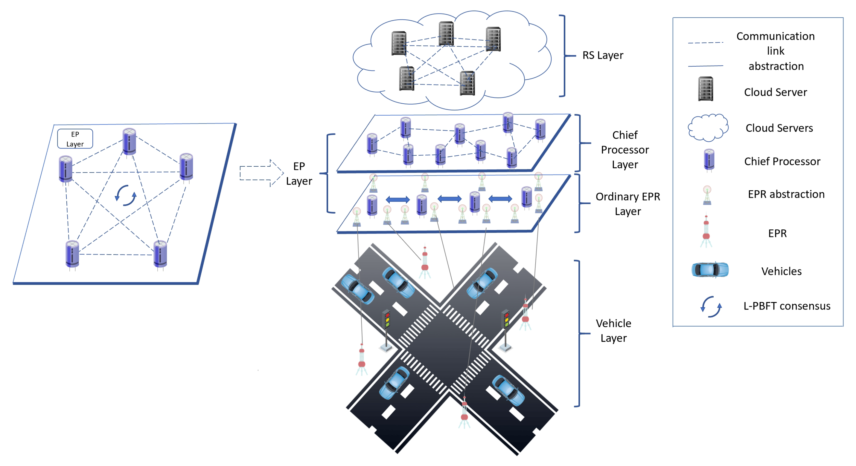
Traditional approaches commonly utilize a central server to cache the blockchain. We propose a Content Sharding mechanism to allow nodes within one group to cache similar blocks and nodes between various groups to cooperatively store the whole blockchain. The ES Layer provides services to vehicles in the form of cooperative search. This pattern can reduce the complexity of the central server to a certain extent, and at the same time improve the response speed of EPRs and balance the network load.

4.1. Group Caching and Data Access Costs

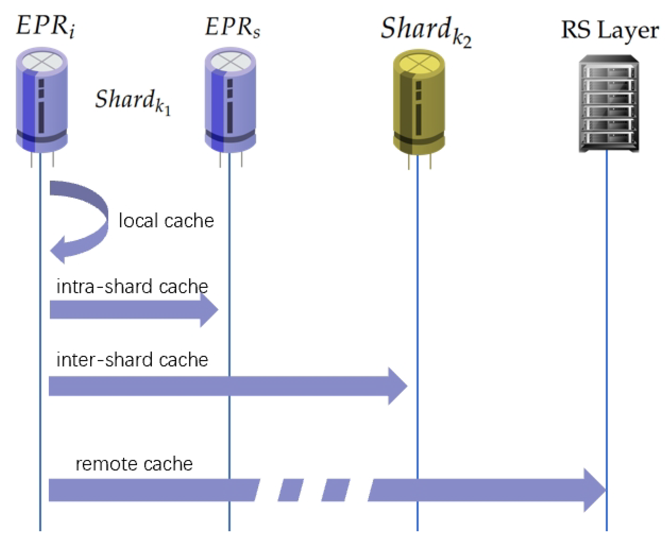
Since the blocks are scattered on different EPRs, the block storage of one EPR may not always be able to fully cover its incoming block query requests. Therefore, EPRs need to cooperate with each other to provide complete services. Different search paths for different cache locations of the blocks are shown in Figure 2. The cost of a node accessing its own storage list is different from the cost of a node forwarding a query through a network request. In order to be able to better describe the above process, we define the cost function for a single data access request, a single EPR in (10):

$${\mho }_{i,j,r}^{\left(\breve{r}\right)}=\left\{\begin{array}{cc}0\hfill & \mathrm{if}\breve{r}\ne i\hfill \\ w_1\hfill & \mathrm{if}\breve{r}=i\&{\check{b}}_j\in {\mathbb{E}}_i\hfill \\ 2w_1+w_2+D_{is}\hfill & \mathrm{if}\breve{r}=i\&{\check{b}}_j\notin {\mathbb{E}}_i\&{\check{b}}_j\in {\mathbb{E}}_s\hfill \\ w_1+w_2+w_3+D_{k_1,k_2}\hfill & \mathrm{if}\breve{r}=i\&{\check{b}}_j\notin {\mathbb{E}}_i\&{\check{b}}_j\in Shar{d}_{k_2}\hfill \\ w_4\hfill & \mathrm{if}\breve{r}=i\&{\check{b}}_j\in \mathrm{RS}\mathrm{Layer}\hfill \end{array}\right.$$

(10)

where ${\check{b}}_j$ is a block with sequence number j and $1\le j\le J$, where J is the total number of blocks. Then, the blocks caching in $EP{R}_i$ can be denoted as ${\mathbb{E}}_i=\{{\check{b}}_j\mid {\check{b}}_{j}inEP{R}_i\}$. ${\widehat{\mathit{Req}}}_r$ stands for request with sequence number r and $1\le r\le R$, where R is the total number of requests. $\breve{r}$ is the index of EPR being requested, where $1\le \breve{r}\le R$. In $Shar{d}_{k_1}$, $EP{R}_s$ is one of the neighbors of $EP{R}_i$, which caches ${\check{b}}_j$.

There exist five search paths for various cache locations. $w_1$ and $w_2$ stand for the cost of search local and neighbor cache; $w_3$ stands for the cost of the forward request to another $Shar{d}_{k_2}$; $w_4$ stands for the cost of the offered help from remote storage. $D_{is}$ and $D_{k_1,k_2}$ represent the transmission cost on short links between $EP{R}_i,EP{R}_s$ in the same $Shar{d}_{k_1}$ and long links between $Shar{d}_{k_1}$ and $Shar{d}_{k_2}$.

Since the TDVS algorithm takes into account the topology, there exists $w_1<w_2\ll w_3\ll w_4$. Hence, the cost of a single request grows larger as the block cache location becomes farther.

4.2. Content Sharding

In the context of network data caching, whether a block is stored on a EPR depends on how often the block is accessed and how much it costs to query or forward. This process requires continuous learning and revision of the system. So, we employ the Traffic-Data-based Genetic Algorithm (TDGA) to solve the block cache location problem. The GA simulates the process of block caching as the evolution of a population. In the temporal dimension, the population keeps reproducing to adapt to the data access patterns; in the spatial dimension, the individuals within the population interact and collaborate with each other, exploring to find an excellent evolutionary direction. Scholars have already been using Genetic Algorithms (GAs) to solve caching problems. For example, Ref. [32] introduces a self-tuning cache replacement policy based on which the future request of a cache block is forecast based on its access pattern. The proposed policy constantly balances among the potential attributes of the object in the cache memory: recency, frequency, size, and time. However, Ref. [32] focuses on the traditional cache policy rather than the blockchain field. The TDGA combines the GA and blockchain concept tightly to realize an effective block caching strategy. The pseudocode of the GA is Algorithm 3.

We use ${\mathbb{E}}_k$ to stand for a set of cached blocks in $Shar{d}_k$. Thus, an individual of the GA is denoted as (11), where $1\le m\le M$ and M is the population size:

$$x_m=\{{\mathbb{E}}_k\mid 1\le k\le K\}$$

(11)

The fitness of this individual is (12):

$${\zeta }_m=\frac{1}{{\sum }_{r=1}^R{\sum }_{j=1}^J{\sum }_{i=1}^I{\mho }_{i,j,r}^{\left(\breve{r}\right)}}$$

(12)

Thus, the population and its fitness set can be represented as (13):

$$\mathbb{X}=\{x_m\mid 1\le m\le M\},\mathbb{F}=\{{\zeta }_m\mid 1\le m\le M\}$$

(13)

Algorithm 3 Pseudocode for GA.

Input:  population size M, mutation possibility $\xi$, crossover possibility $\eta$, convergence threshold $ϵ$, maximum iterations $\widehat{\mathbb{T}}$, total number of blocks J Output:  best individual $x_{max}$  1: current timer t ← 0  2: ${\mathbb{X}}^{\left(0\right)}$← random generate M individuals  3: ${\mathbb{F}}^{\left(0\right)}\leftarrow ⌀$  4: $x_{max}\leftarrow ⌀$, ${\zeta }_{max}\leftarrow {{\zeta }_{max}}^{\left(0\right)}\leftarrow$ 0  5: for  ${x_m}^{\left(0\right)}\in {\mathbb{X}}^{\left(0\right)}$do  6:       ${{\zeta }_m}^{\left(0\right)}$← FC(${x_m}^{\left(0\right)}$)  7:       ${\mathbb{F}}^{\left(0\right)}\leftarrow {\mathbb{F}}^{\left(0\right)}\cup \left\{{{\zeta }_m}^{\left(0\right)}\right\}$  8: end for  9: while t $<\widehat{\mathbb{T}}$ do 10:      ${\mathbb{X}}^{(t+1)}$, ${\mathbb{F}}^{(t+1)}$← RWS(${\mathbb{X}}^{\left(t\right)}$, ${\mathbb{F}}^{\left(t\right)}$) 11:      for $m_1$ and $m_2$ from 1 to M with step = 2 do 12:          ${x_{m_1}}^{(t+1)}$ and ${x_{m_2}}^{(t+1)}$ from ${\mathbb{X}}^{(t+1)}$ 13:          $r_1$ = random float $\in [0,1)$ 14:          $r_2$ = random float $\in [0,1)$ 15:          if $r_1<\eta$ then 16:              ${\widehat{x_{m_1}}}^{(t+1)}$, ${\widehat{x_{m_2}}}^{(t+1)}$← CO(${x_{m_1}}^{(t+1)}$, ${x_{m_2}}^{(t+1)}$) 17:          else if $r_2<\xi$ then 18:              ${\widehat{x_{m_1}}}^{(t+1)}$← MU(${x_{m_1}}^{(t+1)}$, J) 19:              ${\widehat{x_{m_2}}}^{(t+1)}$← MU(${x_{m_2}}^{(t+1)}$, J) 20:          end if 21:          ${x_{m_1}}^{(t+1)}\leftarrow {\widehat{x_{m_1}}}^{(t+1)}$ 22:          ${x_{m_2}}^{(t+1)}\leftarrow {\widehat{x_{m_2}}}^{(t+1)}$ 23:     end for 24:     ${\mathbb{F}}^{(t+1)}\leftarrow ⌀$ 25:     for ${x_m}^{(t+1)}\in {\mathbb{X}}^{(t+1)}$ do 26:           ${{\zeta }_m}^{(t+1)}$← FC(${x_m}^{(t+1)}$) 27:           ${\mathbb{F}}^{(t+1)}\leftarrow {\mathbb{F}}^{(t+1)}\cup \left\{{{\zeta }_m}^{(t+1)}\right\}$ 28:     end for 29:     ${x_{max}}^{(t+1)}$ with ${{\zeta }_{max}}^{(t+1)}$ = $\underset{{x_m}^{(t+1)}\in {\mathbb{X}}^{(t+1)}}{argmax}\left({{\zeta }_m}^{(t+1)}\right)$ 30:     ${x_{min}}^{(t+1)}$ with ${{\zeta }_{min}}^{(t+1)}$ = $\underset{{x_m}^{(t+1)}\in {\mathbb{X}}^{(t+1)}}{argmin}\left({{\zeta }_m}^{(t+1)}\right)$ 31:     if ${\zeta }_{max}<{{\zeta }_{max}}^{(t+1)}$ then 32:          if ${{\zeta }_{max}}^{(t+1)}-{\zeta }_{max}<ϵ$ then 33:              BREAK 34:          end if 35:          ${\zeta }_{max}\leftarrow {{\zeta }_{max}}^{(t+1)}$ 36:          $x_{max}\leftarrow {x_{max}}^{(t+1)}$ 37:      end if 38:      t ← t + 1 39: end while 40: return$x_{max}$

In Algorithm 3, Roulette Wheel Selection (RWS) is one of the selection methods and follows the definition in [33]. The probability of an individual being selected is proportional to the size of its fitness. The Fitness Calculation (FC) function refers to (12).

The Crossover (CO) function follows the rule of two-point crossover in [34], shown in Algorithm 4. There are some well-known crossover operators, such as single point, two point, k point, uniform, and so on. As concluded in [34], these methods both have pros and cons. Single-point crossover is easy to implement, but it lacks diversity. Two-point crossover has a similar effect, but it is applicable on small subsets. Uniform crossover has better recombination potential but still lacks diversity. Other crossover solutions have redundancy issues and premature convergence.

Based on real tests, we apply two-point crossover in our design. There are two reasons:

• Two-point crossover has lower complexity and cost. Considering the previously mentioned node shard mechanism, the entities that are actually involved in the genetic algorithm are drastically reduced after partitioning. In other words, the size of $x_m$ in the cache reallocation is reduced from I (total number of EPRs) to K (total number of shards), where K ≪ I. Thus, two-point crossover with lower complexity and operating cost is well suited to the model of this paper.
• Two-point crossover makes sense in the context of the real world. The chromosome designed in this paper is a list of blocks cached by all shards. The cached list is actually equivalent to a single gene. The crossing of two individuals can be considered as exchanging a useful cache with each other. Thus, two-point crossover makes physical sense.

Algorithm 4 Pseudocode for CO.

Input:  two individual ${x_{m_1}}^{(t+1)}$ and ${x_{m_2}}^{(t+1)}$ Output:  two individual after crossover ${\widehat{x_{m_1}}}^{(t+1)}$ and ${\widehat{x_{m_2}}}^{(t+1)}$ 1: $inde{x}_1$ = random integer $\in [0,K)$ 2: $inde{x}_2$ = random integer $\in [0,K)$ 3: if  $inde{x}_1>inde{x}_2$ then 4:       switch $inde{x}_1$ and $inde{x}_2$ 5: end if 6: switch ${\mathbb{E}}_{inde{x}_1}$ in ${x_{m_1}}^{(t+1)}$ and ${\mathbb{E}}_{inde{x}_2}$ in ${x_{m_2}}^{(t+1)}$ 7: ${\widehat{x_{m_1}}}^{(t+1)}$←${x_{m_1}}^{(t+1)}$ after switch 8: ${\widehat{x_{m_2}}}^{(t+1)}$←${x_{m_2}}^{(t+1)}$ after switch 9: return ${\widehat{x_{m_1}}}^{(t+1)}$, ${\widehat{x_{m_2}}}^{(t+1)}$

There are also many types of mutation operations. Based on the best combination of operations mentioned in [34], we choose to use the value displacement mutation to fit the two-point crossover above, shown in Algorithm 5.

Algorithm 5 Pseudocode for MU.

Input:  an individual ${x_m}^{(t+1)}$, total number of blocks J Output:  an individual after mutation ${\widehat{x_m}}^{(t+1)}$ 1: $inde{x}_1$ = random integer $\in [0,K)$ 2: $inde{x}_2$ = random integer $\in [0,\mid {\mathbb{E}}_{inde{x}_1}\mid )$ 3: $inde{x}_3$ = random integer $\in [0,J)$ 4: changes the block in ${\mathbb{E}}_{inde{x}_1}$ with position $inde{x}_2$ into ${\check{b}}_{index3}$ 5: ${\widehat{x_m}}^{(t+1)}$←${x_m}^{(t+1)}$ after change 6: return  ${\widehat{x_m}}^{(t+1)}$

In the area of selecting ratios of crossover and mutation, recent scholars have used different parameters. Ref. [35] tests the crossover rate from 0.1 to 0.9 and finds out that the best crossover rates are 0.5 and 0.6. Ref. [36] sets the mutation rate to be 0.25. Ref. [37] sets the crossover rate = 0.7 and mutation rate = 0.01 to 0.04. Ref. [38] suggests that the general value of the crossover probability is 0.4 to 0.99, and the range of mutation probability is 0.0001 to 0.1. Ref. [39] sets the crossover rate = 0.8 and mutation rate = 0.01. Ref. [40] sets the crossover rate = 0.5 and mutation rate = 0.01. Ref. [41] sets the crossover rate = 0.7 and mutation rate = 0.3.

In the actual optimization, we find out that the combination of the crossover rate = 0.4 and mutation rate = 0.5 can achieve a more stable and high fitness value. The crossover rate seems to be smaller while the mutation rate seems to be larger than the settings described above. Such a choice is based on considerations of both scale and the experimental results. On the one hand, the crossover part of a chromosome is $\frac{2}{K}$ of the individual size, which is a relatively large proportion in the case of a smaller value of K. for better management. This leads to a smaller crossover probability. Moreover, the number of digits involved in the mutation operation is less compared to the number of digits in the whole chromosome ($\frac{1}{\mathrm{individual}\mathrm{size}}$). This leads to a larger mutation probability. On the other hand, based on actual tests and attempts, larger crossover rates and smaller mutation rates lead to high-fitness individual oscillations and difficulty in convergence. Ref. [42] proposes that crossover appears to be more efficient than the mutation in larger population sizes, and the mutation is more efficient in small populations. Taking into account that cache allocation should be highly real time, the population size needs to be scaled down to a smaller range. So under the condition of a small population, the combination of a higher mutation probability and lower crossover probability can obtain better experimental results indeed also in accordance with the theoretical description.

In our design, the crossover and mutation strategies are dichotomous in each iteration. Although most genetic algorithms are used with both of these two, we have observed in real-world tests that using both operations leads to a faster increase in the fitness of the population but inevitably leads to oscillations at the high points as time goes by. Ref. [32] also suggests that crossover and mutation strategies do not work for every chromosome. Ref. [43] makes the same choices: pairs of the permutations are randomly selected, and a crossover operation is conducted between those pairs. Each newly obtained offspring then undergoes either another crossover or a mutation operator. Ref. [44] mentions that only some of the offspring can participate in the mutation. Ref. [45] uses a mutation probability to control for the dichotomy between crossover and mutation operations. Therefore, it is a feasible solution to set the crossover and mutation operations to be alternative for each individual.

We train the population by simulating a set of regular requests such as the fixed frequency of blocks being accessed on the EP Layer. The output $x_{max}$ contains the block lists of each shard.

With sufficient computing resources, the RS Layer integrates the data reported by the lower layer and undertakes GA. The CPs of each shard broadcast the block list issued by the RS Layer to other ordinary nodes within the same shard. One block list is shared within the shard and is the most compatible with the data features of the assigned shard.

Furthermore, EPRs within the same shard will filter the blocks suitable for their service pattern. The filtering principle is based on the relevance degree introduced in the next section.

4.3. Relevance Degree of Blocks on EPRs

EPRs aim to select the blocks that are most valuable to them. Therefore, we define a measurement of the storage priority between a block and a EPR. The Relevance Degree (RD) can influence whether the block can stay or not. Firstly, the presentation of the pattern of the block content and the node being accessed needs to be numerically settled.Then, the relevance between these two is assessed.

Due to the variety of types of on-board applications, the structure and content of data may vary greatly from application to application. However, the way of describing the data of different applications is more likely to have textual descriptions or textual remarks. Therefore, in order to be compatible with the data uploaded and downloaded in the network, we exploit some values relating to keywords to describe a segment of data. Details of the numerical depiction of a segment of data are below.

Firstly, some professional lexical tools or manual methods can be applied to produce a list of words that appear in certain IoV data. Since this part is beyond our scope, it will not be introduced later. We mainly focus on the depiction of a segment of data after structuring and its subsequent evolution. Referring to the implementation of the Term Frequency-Inverse Document Frequency (TF-IDF) method [46], ${\psi }_i$ and ${\rho }_j$ are denoted as the quantitative expression of history requests of $EP{R}_i$ and the content analysis expression of block ${\check{b}}_j$. V is the total number of keywords:

$${\psi }_i=[{\psi }_i^{\left(1\right)},{\psi }_i^{\left(2\right)},\dots ,{\psi }_i^{\left(V\right)}],{\rho }_j=[{\rho }_j^{\left(1\right)},{\rho }_j^{\left(2\right)},\dots ,{\rho }_j^{\left(V\right)}]$$

(14)

The Kullback–Leibler (KL) divergence in [47] and Jensen–Shannon (JS) divergence in [48] are both used for a measurement of how one probability distribution is different from a second. JS divergence has relatively small numerical fluctuations and is symmetrical. Thus, the Relevance Degree between $EP{R}_i$ and ${\check{b}}_j$ is denoted as (16):

$$KL({\psi }_i\Vert {\rho }_j)=\sum _{v=1}^V{\psi }_i^{\left(v\right)}log\frac{{\psi }_i^{\left(v\right)}}{{\rho }_j^{\left(v\right)}},$$

(15)

$$\begin{array}{cc}\hfill RD(EP{R}_i,{\check{b}}_j)=JS({\psi }_i\Vert {\rho }_j)& =\frac{1}{2}KL({\psi }_i\Vert \frac{{\psi }_i+{\rho }_j}{2})+\frac{1}{2}KL({\rho }_j\Vert \frac{{\psi }_i+{\rho }_j}{2})\hfill \\ \hfill \Rightarrow JS({\psi }_i\Vert {\rho }_j)& =\frac{1}{2}\sum _{v=1}^V{\psi }_i^{\left(v\right)}log\frac{2{\psi }_i^{\left(v\right)}}{{\psi }_i^{\left(v\right)}+{\rho }_j^{\left(v\right)}}+\frac{1}{2}\sum _{v=1}^V{\rho }_j^{\left(v\right)}log\frac{2{\rho }_j^{\left(v\right)}}{{\psi }_i^{\left(v\right)}+{\rho }_j^{\left(v\right)}}\hfill \end{array}$$

(16)

EPRs picks the top several blocks closest to them and then add them to the local cache.

4.4. Complexity Analysis

The space complexity ($SC$) of the GA relates to the number of individuals (M) and the individual capacity ($C_1$). The individual capacity relates to the total number of EPRs (I) and the total number of blocks contained in a single EPR ($C_2$). The space complexity of the GA algorithm is given in the following formula:

$$SC=M\times C_1=M\times I\times C_2$$

(17)

The time complexity ($TC$) of the GA relates to the number of iterations ($\widehat{\mathbb{T}}$) and the number of individuals M:

$$TC=\widehat{\mathbb{T}}\times M$$

(18)

Parallelization Process

The TDGA searches for the global optimal solution as much as possible by using a large number of individuals and generations. Therefore, the number of iterations $\widehat{\mathbb{T}}$ and the number of individuals M need to be large enough. For a single node to run the above algorithm, the time complexity and space complexity are indeed high.

However, the crossover and mutation operations designed in this paper involve at most two neighboring individuals. Moreover, these two neighboring individuals can be determined immediately after the start of each iteration. Therefore, the crossover and mutation operations at each round of iteration can be processed in parallel.

It is a reasonable assumption that all EPRs participate in the algorithm computation. For each computation node, the number of individuals to be processed per iteration is $\frac{M}{I}$, where I represents the total number of EPRs. Each computation node can perform the crossover, mutation and updating of fitness on each set of individuals. Finally, the I computation results are aggregated to the main process, and the new population is derived using the RWS mentioned above in [33]. For a single computation node, the space and time complexities are reduced to $\widetilde{SC}$ and $\widetilde{TC}$ below:

$$\widetilde{SC}=\frac{M}{I}\times C_1=\frac{M}{I}\times I\times C_2=M\times C_2$$

(19)

$$\widetilde{TC}=\widehat{\mathbb{T}}\times \frac{M}{I}=O\left(\widehat{\mathbb{T}}\right)$$

(20)

There are some recommendations of the chosen M in the literature. Ref. [49] believes that population size = 20 is enough. Ref. [35] tests the population size from 20 to 200 and generation size from 200 to 500. The results show that a higher number of generations with a smaller population size performs better. And the best combination is a population size of 50 and generation size of 100. Refs. [39,40,50] set the population size to be 100. Ref. [42] refers that a population size of less than about 1000 chromosomes has positive effects. Ref. [51] conducts a series of experiments to prove that for functions with a large number of dimensions, a size of 800 individuals with a number of generations equal to 1000 seems to be the most favorable. Thus, M can be set to about 300, practically (between 20 and 1000).

At the time of writing this paper, the total number of Bitcoin blocks is between 800,000 and 900,000. Thus, a 900,000-bit array can be used to store the block list within one node. Therefore, $C_2$ is set to be 900,000 bits.

Referring to (19), $\widetilde{SC}=M\times C_2=33.75$ MB, which is far less than the memory of the fourth-generation Raspberry Pi (8GB) deployed in the next experiment section.

The total number of EPRs has the same order of magnitude as M, which causes $\frac{M}{I}$ in (20) to be a small constant compared to $\widehat{\mathbb{T}}$. As for the chosen generation number $\widehat{\mathbb{T}}$, we were not able to find a unified standard figure. Refs. [36,39,50] set the generation size to be 100. Ref. [37] sets the value to be 200. Refs. [40,41] set it to be 1000. Moreover, in the next section, we also find that the highest fitness holds up at about 1000 generations. As a result, $\widehat{\mathbb{T}}$ can be set to 1000 in general, which is also affordable for Raspberry Pi (8 GB) deployed in the next experiment section.

The process of the TDGA has a short time interval, or can be triggered at regular intervals or under other suitable conditions. If the frequency of data updated is high under the current road conditions, then the task of data analysis is frequently added to the schedule of the RS Layer with high priority, which in turn leads to real-time changes in the block storage of the EPRs to meet the rapidly changing road environment. As mentioned earlier, the resource of the RS Layer is much better than the other two lower layers. Therefore, under the impetus of the rapidly updated and generated data, the increasing pressure of the other two lower layers is mainly manifested in communication. Pressure on the RS Layer is obviously greater than that of the other two layers, which will not reflect on the response speed of IoV services. In summary, the complexity of the TDGA can endure the rapid road information changes under the above algorithms.

5. Experiments and Analysis

Since the framework is based on the IoV environment, the experimental environment uses the fourth-generation Raspberry Pi (RP) and Mac host (MH) to simulate the IoV environment. Mac has 2.3 GHz of CPU performance and 16 GB of memory space. Raspberry Pi has 1.5 GHz of CPU performance and 8 GB of memory space. The Java programming language is used to implement the framework and the comparison tests. The experimental environment uses a 5G router from TP_LINK as a routing relay.

The experimental data use a combination of simulated data from the SUMO (1.19.0) application [52], highD dataset [53] and some locally generated random data. The SUMO (Simulation of Urban Mobility) application is an open-source transportation simulation software. SUMO provides interfaces to set up the structure of the road topology and configure the speed and number of vehicles for each road. The HighD dataset is a large natural vehicle trajectory data for German highways. THe HighD dataset contains the speed and positions of vehicles collected at fixed time intervals. Simulated data are used for the framework simulation test, and the locally random data are used to simulate directionally oriented data interest pointing, i.e., different sections of the road have different data characteristics as mentioned before. All data are stored in the blocks. The block parameters designed in this experiment are shown in

Table 2. Block parameters.

Total Blocks	Block Capacity	Transaction Size	Link Cost
13,333	16 transactions	≤64 bytes	random floats from 5 to 10 1

¹ Dimensionless link cost for convenience of calculation.

.

Block parameters are slightly different from the traditional Bitcoin block. The size of a traditional Bitcoin block is about 1 MB to 4 MB, and the average Bitcoin transaction is about 250 bytes [25]. Due to the limitations of the equipment used for the simulation experiments, we reduce both the transaction and block size.

5.1. Sharding Result Comparison

TDVS uses both traffic flow data and topology information to group nodes. The purpose is to classify nodes that communicate frequently or collect the same tendency of data in the same group. In order to verify that the division of TDVS is indeed effective, this paper uses comparative experiments to verify the partition effect.

HighD data with 171 time episodes are applied to the following experiments. The comparison algorithm uses K-means partition (KMP) and geographical partition (GP) [53]. Although the HighD dataset contains geographical information, the number of collection points is not suitable for our study, so we divide 169 areas according to the span of latitude and longitude to create 169 virtual ERPs across 4 lanes, which is in accordance with the description of HighD. GP is designed for grouping nodes based only on their geographical location. KMP [54] is a division-based clustering algorithm that divides the sample features into classes according to their Euclidean square distance. K is set to 4 in order to match the HighD dataset. Thus, KMP groups EPRs based only on their traffic data.

The quality of partition result is measured by four metrics: K-means Loss function (KML) and Negative Compactness (NC) [55], Havrda–Charvat Entropy (HCE) [56], and Modularity Value (MV) [57]. Figure 3, Figure 4, Figure 5 and Figure 6 are line charts for these four values.

KML and HCE are related to the node attribute values. Smaller values indicate that the node attribute vectors are more similar in the same shard, whereas the node attribute vectors in different shards are more divergent. NC and MV are related to the node topology. Small NC and large MV both indicate that nodes in the same shard are tightly connected, while nodes in different shards are sparsely connected.

5.2. Cache Comparison

The TDGA utilizes the link cost and relevance degree to allocate blocks into appropriate shards. In this paper, we test the latency of EPRs of processing vehicle requests to corroborate the usability of TDGA. The comparison algorithms use Frequency(or Popularity)-Based Caching (FBC) [58], Load-Balancing-based Caching (LBC) [58] and Digital Twin Collaborative Caching (DTCC) [59] mechanisms. FBC allocates blocks based on the frequency of requests on ERPs or, in other words, the percentage of the number of times that EPR has been requested out of the total number of requests globally; the LBC algorithm focuses on the balanced capacity of EPRs.

The DTCC algorithm originally deals with the problems of local cache and the edge cache model. DTCC has strong similarities to the problem described in this paper, so it is used as a comparison algorithm. However, its evaluation formula cannot be directly used in the design context of this paper, so we make a little modification as follows:

• We modify the embeddings of the cache content and task into the TF-IDF value of blocks and EPRs.
• We change the frequency of the occurrence of the task and the mean frequency of the occurrence of complete tasks into the query frequency of blocks on EPRs.
• We change the consumption of computing tasks into the link cost shown in Table 2.
• Since the original description of caching in [59] is not very detailed, we have tried as much as possible to reproduce the author’s ideas. Our reconstruction scheme is as follows: after each request, EPRs add the block of the current request to the local memory; after every 100 requests, EPRs delete the blocks with the lowest evaluated value in the local memory (we set 10% of the total local cache); and for every 100 requests, EPRs swap the local memories with each other to delete overlapping and low evaluated value blocks.

The above mechanism is named the DTCC-like mechanism or DTCCL in the following descriptions. TDGA, FBC and DTCCL are conducted after every 100 requests, and LBC is conducted after every request. The crossover rate is set to 0.4, and the mutation rate is set to 0.5.

The following initial experimental conditions are the same for all three algorithms:

• The number of EPRs is 10, and the capacity of each EPR is 100 blocks. The cost of links is the same, which is randomly generated in advance. The topology of EPRs is shown in Figure 7. This is a basic road model containing horizontal and vertical roads and intersections. All EPRs are divided into K = 3 shards with three colors (blue for the up three roads, orange for the middle four roads and green for the bottom three roads). More complex roadway models would indeed be more convincing, and that will be our future works. In this paper, the usage of a basic but effective road model is sufficient to show the effect of the algorithm we designed. The network schematic is given in Figure 8.
• There exists a fixed list of requests for simulating the historical request for blocks on EPRs. The list is recycled and can be used to simulate regular request tendencies, such as requests on two adjacent days that may be extremely similar.

Each EPR does not contain any cache after the initial session of the system. As the vehicle nodes keep issuing query requests, the EPRs return query results to the vehicles based on different caching patterns. The nodes also record the query time and update the local cache. The main java interfaces applied are InetAddress, MulticastSocket, DatagramPacket. We also apply Thread, ConcurrentLinkedQueue and ExecutorService to realize a multi-thread EPR in order to process requests as much as possible.

The actual IoV is a mixed environment with both wired and wireless network transmission. Thus, this simulation experiment employs wired and wireless links at the same time. Based on the various hardware implementations and transmission types corresponding to various types of nodes, we classify them into five modes as shown in

Table 3. Five modes.

	Mode 1	Mode 2	Mode 3	Mode 4	Mode 5
EP Layer	RP	RP	RP	RP	MH
RS Layer	RP	RP	MH	MH	MH
Link Type	wireless	wired	wireless	wired	MH local

.

The latency for a request is defined from the time an ERP receives a request until the EPR obtains the exact block cache for that request. We take the average delays computed by all nodes. Experiment times range from 200 to 1300. The line charts are plotted in Figure 9, Figure 10, Figure 11, Figure 12 and Figure 13. Based on equipment limitations, we have only included the DTCCL comparison data in Figure 13. The trend and the gap can already be clearly seen.

We use data from 200 to 1300 experiment times for two reasons. On the one hand, the number of experiments below 200 is too small to see the effect of the algorithm. On the other hand, after reaching 1300 times, the trend of the line graph tends to be flat, and the data of the line graph from 200 to 1300 times already show the obvious effect of the experiments, so there is not much need to continue to increase the number of experiments above 1300 times.

Experimental results show that the TDGA does outperform the other two algorithms in terms of delay. With the joining of RP, the overall delay is increased. Due to the gap in the performance of MH and RP, the more MH that takes up the work, the lower the latency. It is clear that there is a substantial reduction in the delay in the case of all host nodes. The case of all RP nodes has the highest delay. The performance of the wired network connection is overall higher than the performance of the wireless connection; this is due to the speed of transferring the data, and the package delivery rate becomes faster.

As mentioned earlier, caches may be available locally, in other shards or at remote services. The location statistics of the cache hit times for the three algorithms are shown in the following Figure 14, Figure 15, Figure 16, Figure 17, Figure 18 and Figure 19. Moreover, based on the equipment limitations, we only included the DTCCL comparison data in Figure 19. The trend and the gap can also already be clearly seen.

The similarity in the trend of the five line graphs is due to the fact that the different modes only affect the delay rather than the hit rate. The hit rate is related to the caching algorithm used. As we can be seen from the trend, the TDGA algorithm seeks as little help as possible from other shards or remote services.

Defining the ratio of cache miss as the ratio of intra-group cache requests and remote services cache requests to the total number of requests, the following

Table 4. Cache miss ratio for Mode 1.

	200	300	400	500	600	700	800	900	1000	1100	1200	1300
TDGA	0.2300	0.2866	0.2975	0.3020	0.3233	0.3271	0.3262	0.3411	0.3300	0.3372	0.3283	0.3453
FBC	0.4750	0.5733	0.5625	0.5640	0.6300	0.5900	0.6150	0.5966	0.6140	0.6018	0.5975	0.6123
LBC	0.5150	0.6600	0.6325	0.6560	0.6733	0.6985	0.7200	0.7388	0.7090	0.7272	0.7016	0.7184

,

Table 5. Cache miss ratio for Mode 2.

	200	300	400	500	600	700	800	900	1000	1100	1200	1300
TDGA	0.2550	0.2567	0.2950	0.3000	0.3167	0.3014	0.3263	0.3378	0.3400	0.3309	0.3392	0.3338
FBC	0.4750	0.5633	0.5650	0.5800	0.5817	0.5643	0.5913	0.6178	0.6410	0.6236	0.6217	0.6308
LBC	0.5050	0.5500	0.6575	0.7160	0.7267	0.6686	0.6888	0.7211	0.7320	0.7236	0.7300	0.7423

,

Table 6. Cache miss ratio for Mode 3.

	200	300	400	500	600	700	800	900	1000	1100	1200	1300
TDGA	0.2050	0.2967	0.3125	0.2900	0.3167	0.3329	0.3338	0.3344	0.3320	0.3355	0.3375	0.3346
FBC	0.4400	0.5767	0.4950	0.5600	0.6233	0.6029	0.6300	0.5922	0.5900	0.6073	0.6142	0.6431
LBC	0.5950	0.6100	0.6275	0.6680	0.7117	0.7200	0.7175	0.7200	0.7340	0.7300	0.7208	0.7346

,

Table 7. Cache miss ratio for Mode 4.

	200	300	400	500	600	700	800	900	1000	1100	1200	1300
TDGA	0.2700	0.2900	0.2875	0.3320	0.3067	0.3229	0.3350	0.3156	0.3320	0.3364	0.3375	0.3323
FBC	0.4050	0.5733	0.5900	0.6280	0.5683	0.5929	0.5975	0.6222	0.6340	0.6073	0.6275	0.6469
LBC	0.6500	0.6300	0.6325	0.6820	0.6883	0.7143	0.7000	0.7256	0.7010	0.7055	0.7117	0.7238

and

Table 8. Cache miss ratio for Mode 5.

	200	300	400	500	600	700	800	900	1000	1100	1200	1300
TDGA	0.2400	0.2967	0.3075	0.3000	0.3117	0.3429	0.3400	0.3344	0.3350	0.3355	0.3350	0.3277
FBC	0.4650	0.6100	0.5925	0.5500	0.5733	0.6086	0.6275	0.6411	0.6110	0.6327	0.6217	0.6500
LBC	0.5850	0.6867	0.6575	0.6680	0.6350	0.6657	0.6913	0.7167	0.7030	0.7073	0.7150	0.7215
DTCCL	0.6050	0.6667	0.6300	0.6280	0.6333	0.6529	0.6638	0.6678	0.6800	0.6491	0.6542	0.6746

show the ratio of cache miss for the five modes. Only in Table 8, we add the DTCCL data due to the equipment limitations.

The TDGA cache miss ratios gradually stabilize due to the fact that the results of the TDGA are more stable and match the tendency of the requested data. The increasing cache miss ratios for the remaining two methods are due to the fact that the consideration of only a single factor is no longer suitable for complex request environments over time. Overall, the TDGA has more reliable performance in terms of both the latency and hit rate. The cache miss rates are relatively similar for all five modes, which is consistent with the results of the previous latency line charts.

6. Conclusions

In this paper, Node Sharding and Content Sharding are introduced into the blockchain-based IoV system. To cope with the difficulties in managing the large number of nodes, this paper designs the TDVS method to organize EPRs into different groups. TDVS relies on traffic data of both a temporal and spatial nature. Grouping the management scheme improves the communication efficiency by reducing the communication complexity. Aiming to alleviate the memory limitation issues of EPRs, this paper aims to optimize the node local memory through the TDGA. Based on the above grouping results, the TDGA gives a more superior data storage scheme based on the link cost and request pattern. Finally, this paper uses the real HighD dataset and SUMO simulation dataset to verify the practicality of the above two proposed methods. The two methods proposed in this paper both outperform the traditional clustering and caching methods in terms of the latency and hit rate.

There are still some shortcomings in this paper on the introduction of blockchain into IoV. We will focus on the improvement of the blockchain consensus mechanism for the grouping scheme and the design of node behavior after the adoption of multiple blockchains.

References

1. Li, X.; Yin, X.; Ning, J. Trustworthy Announcement Dissemination Scheme With Blockchain-Assisted Vehicular Cloud. IEEE Trans. Intell. Transp. Syst. 2023, 24, 1786–1800. [Google Scholar] [CrossRef]
2. Hammoud, A.; Sami, H.; Mourad, A.; Otrok, H.; Mizouni, R.; Bentahar, J. AI, Blockchain, and Vehicular Edge Computing for Smart and Secure IoV: Challenges and Directions. IEEE Internet Things Mag. 2020, 3, 68–73. [Google Scholar] [CrossRef]
3. Guo, Z.; Wang, G.; Li, Y.; Ni, J.; Du, R.; Wang, M. Accountable Attribute-Based Data-Sharing Scheme Based on Blockchain for Vehicular Ad Hoc Network. IEEE Internet Things J. 2023, 10, 7011–7026. [Google Scholar] [CrossRef]
4. Naresh, V.S.; Allavarpu, V.V.L.D.; Reddi, S. Blockchain IOTA Sharding-Based Scalable Secure Group Communication in Large VANETs. IEEE Internet Things J. 2023, 10, 5205–5213. [Google Scholar] [CrossRef]
5. MOBI. The New Economy of Movement. 2021. Available online: https://dlt.mobi/wp-content/uploads/2021/09/MOBI-WP_V3.0.pdf (accessed on 15 July 2021).
6. Ford. Everledger Partners Ford for EV Blockchain Battery Passport Pilot. 2022. Available online: https://www.ledgerinsights.com/everledger-ford-blockchain-ev-battery-passport-recycling/ (accessed on 27 October 2022).
7. Islam, S.; Badsha, S.; Sengupta, S.; La, H.; Khalil, I.; Atiquzzaman, M. Blockchain-Enabled Intelligent Vehicular Edge Computing. IEEE Netw. 2021, 35, 125–131. [Google Scholar] [CrossRef]
8. Wang, S.; Ye, D.; Huang, X.; Yu, R.; Wang, Y.; Zhang, Y. Consortium Blockchain for Secure Resource Sharing in Vehicular Edge Computing: A Contract-Based Approach. IEEE Trans. Netw. Sci. Eng. 2021, 8, 1189–1201. [Google Scholar] [CrossRef]
9. Shen, M.; Lu, H.; Wang, F.; Liu, H.; Zhu, L. Secure and Efficient Blockchain-Assisted Authentication for Edge-Integrated Internet-of-Vehicles. IEEE Trans. Veh. Technol. 2022, 71, 12250–12263. [Google Scholar] [CrossRef]
10. Akrasi-Mensah, N.K.; Agbemenu, A.S.; Nunoo-Mensah, H.; Tchao, E.T.; Ahmed, A.R.; Keelson, E.; Sikora, A.; Welte, D.; Kponyo, J.J. Adaptive Storage Optimization Scheme for Blockchain-IIoT Applications Using Deep Reinforcement Learning. IEEE Access 2023, 11, 1372–1385. [Google Scholar] [CrossRef]
11. Ali, A.; Aadil, F.; Khan, M.F.; Maqsood, M.; Lim, S. Harris Hawks Optimization-Based Clustering Algorithm for Vehicular Ad-Hoc Networks. IEEE Trans. Intell. Transp. Syst. 2023, 24, 5822–5841. [Google Scholar] [CrossRef]
12. Qian, Y.; Jiang, Y.; Hu, L.; Hossain, M.S.; Alrashoud, M.; Al-Hammadi, M. Blockchain-Based Privacy-Aware Content Caching in Cognitive Internet of Vehicles. IEEE Netw. 2020, 34, 46–51. [Google Scholar] [CrossRef]
13. Sang, G.; Chen, J.; Liu, Y.; Wu, H.; Zhou, Y.; Jiang, S. PACM: Privacy-Preserving Authentication Scheme With on-Chain Certificate Management for VANETs. IEEE Trans. Netw. Serv. Manag. 2023, 20, 216–228. [Google Scholar] [CrossRef]
14. Li, X.; Jing, T.; Li, R.; Li, H.; Wang, X.; Shen, D. BDRA: Blockchain and Decentralized Identifiers Assisted Secure Registration and Authentication for VANETs. IEEE Internet Things J. 2023, 10, 12140–12155. [Google Scholar] [CrossRef]
15. Kacem, T. VANET-Sec: A Framework to Secure Vehicular Ad-Hoc Networks Using a Permissioned Blockchain. In Proceedings of the 2023 International Symposium on Networks, Computers and Communications (ISNCC), Doha, Qatar, 23–26 October 2023; pp. 1–6. [Google Scholar] [CrossRef]
16. Anilkumar, S.; Rafeek, J. Soteria: A Blockchain Assisted Lightweight and Efficient Certificateless Handover Authentication Mechanism for VANET. In Proceedings of the 2023 3rd International Conference on Advances in Computing, Communication, Embedded and Secure Systems (ACCESS), Ernakulam, India, 18–20 May 2023; pp. 226–232. [Google Scholar] [CrossRef]
17. Gerrits, L.; Kromes, R.; Verdier, F. A True Decentralized Implementation Based on IoT and Blockchain: A Vehicle Accident Use Case. In Proceedings of the 2020 International Conference on Omni-Layer Intelligent Systems (COINS), Barcelona, Spain, 31 August 2020; pp. 1–6. [Google Scholar] [CrossRef]
18. M, T.; Nawaz, G.M.K. Enabling Secure and Efficient Traffic Data Sharing in VANETs Through a Scalable Blockchain Framework. In Proceedings of the 2023 4th International Conference on Smart Electronics and Communication (ICOSEC), Trichy, India, 20–22 September 2023; pp. 567–573. [Google Scholar] [CrossRef]
19. Xie, Q.; Ding, Z.; Tang, W.; He, D.; Tan, X. Provable Secure and Lightweight Blockchain-Based V2I Handover Authentication and V2V Broadcast Protocol for VANETs. IEEE Trans. Veh. Technol. 2023, 72, 15200–15212. [Google Scholar] [CrossRef]
20. Zhang, C.; Zhang, S.; Zou, X.; Yu, S.; Yu, J.J.Q. Toward Large-Scale Graph-Based Traffic Forecasting: A Data-Driven Network Partitioning Approach. IEEE Internet Things J. 2023, 10, 4506–4519. [Google Scholar] [CrossRef]
21. Ke, S.; Wang, Y.; An, C.; Lu, Z.; Xia, J. Traffic Origin-Destination Flow-Inspired Dynamic Urban Arterial Partition for Coordinated Signal Control Using Automatic License Plate Recognition Data. IEEE Intell. Transp. Syst. Mag. 2024, 16, 132–147. [Google Scholar] [CrossRef]
22. Chougule, A.; Chamola, V.; Hassija, V.; Gupta, P.; Yu, F.R. A Novel Framework for Traffic Congestion Management at Intersections Using Federated Learning and Vertical partitioning. IEEE Trans. Consum. Electron. 2023, 1. [Google Scholar] [CrossRef]
23. Raj, R. Bitcoin Blockchain. Available online: https://intellipaat.com/blog/tutorial/blockchain-tutorial/bitcoin-blockchain/ (accessed on 9 December 2023).
24. Li, L.; Jin, D.; Zhang, T.; Li, N. A Secure, Reliable and Low-Cost Distributed Storage Scheme Based on Blockchain and IPFS for Firefighting IoT Data. IEEE Access 2023, 11, 97318–97330. [Google Scholar] [CrossRef]
25. Bitcoin. Bitcoin: A Peer-to-Peer Electronic Cash System. 2008. Available online: https://bitcoin.org/en/bitcoin-paper (accessed on 31 October 2008).
26. Nartey, C.; Tchao, E.T.; Gadze, J.D.; Yeboah-Akowuah, B.; Nunoo-Mensah, H.; Welte, D.; Sikora, A. Blockchain-IoT peer device storage optimization using an advanced time-variant multi-objective particle swarm optimization algorithm. EURASIP J. Wirel. Commun. Netw. 2022, 2022, 5. [Google Scholar] [CrossRef]
27. Xu, M.; Feng, G.; Ren, Y.; Zhang, X. On Cloud Storage Optimization of Blockchain With a Clustering-Based Genetic Algorithm. IEEE Internet Things J. 2020, 7, 8547–8558. [Google Scholar] [CrossRef]
28. U.S. Department of Transportation. Simplified Highway Capacity Calculation Method for the Highway Performance Monitoring System. Available online: https://www.fhwa.dot.gov/policyinformation/pubs/pl18003/hpms_cap.pdf (accessed on 15 October 2017).
29. Ministry of Housing and Urban-Rural Development. Code for Design of Urban Road Engineering. Available online: https://www.codeofchina.com/standard/CJJ37-2012.html (accessed on 11 November 2012).
30. Gao, X.; Zhao, J.; Wang, M. Modelling the saturation flow rate for continuous flow intersections based on field collected data. PLoS ONE 2020, 15, e0236922. [Google Scholar] [CrossRef]
31. Chen, X.; Er-Rahmadi, B.; Ma, T.; Hillston, J. ParBFT: An Optimized Byzantine Consensus Parallelism Scheme. IEEE Trans. Comput. 2023, 72, 3354–3369. [Google Scholar] [CrossRef]
32. Mourad, A.A.; Mesbah, S.; Mabrouk, T.F. A Novel Approach to Cache Replacement Policy Model Based on Genetic Algorithms. In Proceedings of the 2020 Fourth World Conference on Smart Trends in Systems, Security and Sustainability (WorldS4), London, UK, 27–28 July 2020; pp. 405–411. [Google Scholar] [CrossRef]
33. Lan, Y. Binary-like Real Coding Genetic Algorithm. In Proceedings of the 2023 International Conference on Pattern Recognition, Machine Vision and Intelligent Algorithms (PRMVIA), Beihai, China, 24–26 March 2023; pp. 98–102. [Google Scholar] [CrossRef]
34. Alam, T.; Qamar, S.; Dixit, A.; Benaida, M. Genetic algorithm: Reviews, implementations, and applications. arXiv 2020, arXiv:2007.12673. [Google Scholar] [CrossRef]
35. Nezhad, N.H.M.; Niasar, M.G.; Hagen, C.W.; Kruit, P. Tuning Parameters in the Genetic Algorithm Optimization of Electrostatic Electron Lenses. In Proceedings of the 2023 IEEE MTT-S International Conference on Numerical Electromagnetic and Multiphysics Modeling and Optimization (NEMO), Winnipeg, MB, Canada, 28–30 June 2023; pp. 170–173. [Google Scholar] [CrossRef]
36. Kronberger, G. Local Optimization Often is Ill-conditioned in Genetic Programming for Symbolic Regression. In Proceedings of the 2022 24th International Symposium on Symbolic and Numeric Algorithms for Scientific Computing (SYNASC), Hagenberg/Linz, Austria, 12–15 September 2022; pp. 304–310. [Google Scholar] [CrossRef]
37. Xue, B.; Lyu, Y.; Ji, B.; Wang, W. Genetic Algorithm-Based Iterative Channel Parameter Estimation Method. In Proceedings of the 2023 IEEE 6th International Conference on Electronic Information and Communication Technology (ICEICT), Qingdao, China, 21–24 July 2023; pp. 677–680. [Google Scholar] [CrossRef]
38. Fang, L. Research on Evaluation Algorithm of Roundness Measurement Data Based on Adaptive Genetic Algorithm. In Proceedings of the 2023 IEEE 7th Information Technology and Mechatronics Engineering Conference (ITOEC), Chongqing, China, 15–17 September 2023; Volume 7, pp. 938–942. [Google Scholar] [CrossRef]
39. Xia, W.; Shi, L.; Zhang, R.; Zhang, J.; Zhao, J. A Co-Evolutionary Genetic Algorithm Based on Improved K-Means Clustering. In Proceedings of the 2023 8th International Conference on Image, Vision and Computing (ICIVC), Dalian, China, 27–29 July 2023; pp. 813–818. [Google Scholar] [CrossRef]
40. Zhao, Z.; Chen, M.; Wu, Q.; Chi, X.; Lin, W.; Zhang, B.; Wang, J. An improved RNA genetic algorithm without mutation operation in the later stage. In Proceedings of the 2022 China Automation Congress (CAC), Xiamen, China, 25–27 November 2022; pp. 4787–4792. [Google Scholar] [CrossRef]
41. Raj, B.; Ahmedy, I.; Idris, M.Y.I.; Noor, R.M. A Hybrid Sperm Swarm Optimization and Genetic Algorithm for Unimodal and Multimodal Optimization Problems. IEEE Access 2022, 10, 109580–109596. [Google Scholar] [CrossRef]
42. Melikyan, V.; Harutyunyan, A.; Davtyan, V.; Revazyan, D.; Harutyunyan, G. Tuning Genetic Algorithm Parameters for Placement of Integrated Circuit Cells. In Proceedings of the 2023 IEEE East-West Design & Test Symposium (EWDTS), Batumi, Georgia, 22–25 September 2023; pp. 1–4. [Google Scholar] [CrossRef]
43. Awad, A.; Hawash, A.; Abdalhaq, B. A Genetic Algorithm (GA) and Swarm-Based Binary Decision Diagram (BDD) Reordering Optimizer Reinforced With Recent Operators. IEEE Trans. Evol. Comput. 2023, 27, 535–549. [Google Scholar] [CrossRef]
44. Faridoon, F.; Ali, R.H.; Ul Abideen, Z.; Shahzadi, N.; Ijaz, A.Z.; Arshad, U.; Ali, N.; Imad, M.; Nabi, S. Prediction of Polycystic Ovary Syndrome Using Genetic Algorithm-driven Feature Selection. In Proceedings of the 2023 International Conference on IT and Industrial Technologies (ICIT), Chiniot, Pakistan, 9–10 October 2023; pp. 1–6. [Google Scholar] [CrossRef]
45. Yang, F.; Tian, Z. MRPGA: A Genetic-Algorithm-based In-network Caching for Information-Centric Networking. In Proceedings of the 2021 IEEE 29th International Conference on Network Protocols (ICNP), Dallas, TX, USA, 1–5 November 2021; pp. 1–6. [Google Scholar] [CrossRef]
46. Ngan, S.C.H.; Lee, M.J.; Khor, K.C. Automating Conference Paper Assignment Using Classification Algorithms Incorporated with TF-IDF Vectorisation. In Proceedings of the 2023 IEEE Symposium on Industrial Electronics & Applications (ISIEA), Kuala Lumpur, Malaysia, 15–16 July 2023; pp. 1–6. [Google Scholar] [CrossRef]
47. Bouhlel, N.; Rousseau, D. Exact Rényi and Kullback–Leibler Divergences Between Multivariate t-Distributions. IEEE Signal Process. Lett. 2023, 30, 1672–1676. [Google Scholar] [CrossRef]
48. Ulger, F.; Yuksel, S.E.; Yilmaz, A.; Gokcen, D. Fine-Grained Classification of Solder Joints With alfa-Skew Jensen–Shannon Divergence. IEEE Trans. Compon. Packag. Manuf. Technol. 2023, 13, 257–264. [Google Scholar] [CrossRef]
49. Benecke, T.; Mostaghim, S. Effects of Optimal Genetic Material in the Initial Population of Evolutionary Algorithms. In Proceedings of the 2023 IEEE Symposium Series on Computational Intelligence (SSCI), Mexico City, Mexico, 5–8 December 2023; pp. 1386–1391. [Google Scholar] [CrossRef]
50. Zhang, W.; Hua, D.L.; Li, S.H.; Ren, Z.; Yu, Z.L. An improved genetic programming algorithm based on bloat control. In Proceedings of the 2023 4th International Conference on Big Data & Artificial Intelligence & Software Engineering (ICBASE), Nanjing, China, 25–27 August 2023; pp. 406–413. [Google Scholar] [CrossRef]
51. Asmae, E.B.; Sanae, H.; Bachir, B. A Study of Genetic Algorithm Parameterization via a Benchmark of Test Functions. In Proceedings of the 2023 3rd International Conference on Innovative Research in Applied Science, Engineering and Technology (IRASET), Mohammedia, Morocco, 18–19 May 2023; pp. 1–5. [Google Scholar] [CrossRef]
52. Alvarez Lopez, P.; Behrisch, M.; Bieker-Walz, L.; Erdmann, J.; Flötteröd, Y.P.; Hilbrich, R.; Lücken, L.; Rummel, J.; Wagner, P.; Wießner, E. Microscopic Traffic Simulation using SUMO. In Proceedings of the 2018 IEEE Intelligent Transportation Systems Conference (ITSC), Maui, HI, USA, 4–7 November 2018; pp. 2575–2582. [Google Scholar]
53. Krajewski, R.; Bock, J.; Kloeker, L.; Eckstein, L. The highD Dataset: A Drone Dataset of Naturalistic Vehicle Trajectories on German Highways for Validation of Highly Automated Driving Systems. In Proceedings of the 2018 21st International Conference on Intelligent Transportation Systems (ITSC), Maui, HI, USA, 4–7 November 2018; pp. 2118–2125. [Google Scholar] [CrossRef]
54. Žalik, K.R.; Žalik, M. Comparison of K-Means, K-Means++, X-Means and Single Value Decomposition for Image Compression. In Proceedings of the 2023 27th International Conference on Circuits, Systems, Communications and Computers (CSCC), Rhodes (Rodos) Island, Greece, 19–22 July 2023; pp. 295–301. [Google Scholar] [CrossRef]
55. Bu, Z.; Wu, Z.; Cao, J.; Jiang, Y. Local Community Mining on Distributed and Dynamic Networks From a Multiagent Perspective. IEEE Trans. Cybern. 2016, 46, 986–999. [Google Scholar] [CrossRef]
56. Shi, Y.; Wu, Y.; Shang, P. Research on weighted Havrda–Charvat’s entropy in financial time series. Phys. A Stat. Mech. Its Appl. 2021, 572, 125914. [Google Scholar] [CrossRef]
57. Yang, T.H.; Huang, C.Y. Improving Software Modularization Quality Through the Use of Multi-Pattern Modularity Clustering Algorithm. In Proceedings of the 2023 IEEE 23rd International Conference on Software Quality, Reliability, and Security (QRS), Chiang Mai, Thailand, 22–26 October 2023; pp. 696–706. [Google Scholar] [CrossRef]
58. Zhang, Z.; Lung, C.H.; Wei, X.; Chen, M.; Chatterjee, S.; Zhang, Z. In-Network Caching for ICN-Based IoT (ICN-IoT): A Comprehensive Survey. IEEE Internet Things J. 2023, 10, 14595–14620. [Google Scholar] [CrossRef]
59. Song, Y.; Shenyun. Video Stream Caching Based on Digital Twin Cooperative Caching. In Proceedings of the 2023 IEEE International Symposium on Broadband Multimedia Systems and Broadcasting (BMSB), Beijing, China, 14–16 June 2023; pp. 1–5. [Google Scholar] [CrossRef]
Figure 1. Three-tier IoV.
Electronics 13 00560 g001
Figure 2. Different search paths due to different cache location.
Electronics 13 00560 g002
Figure 3. K-means Loss function (KML).
Electronics 13 00560 g003
Figure 4. Negative Compactness (NC).
Electronics 13 00560 g004
Figure 5. Havrda–Charvat Entropy (HCE).
Electronics 13 00560 g005
Figure 6. Modularity Value (MV).
Electronics 13 00560 g006
Figure 7. Topology of EPRs.
Electronics 13 00560 g007
Figure 8. Network schematic.
Electronics 13 00560 g008
Figure 9. Latency for Mode 1.
Electronics 13 00560 g009
Figure 10. Latency for Mode 2.
Electronics 13 00560 g010
Figure 11. Latency for Mode 3.
Electronics 13 00560 g011
Figure 12. Latency for Mode 4.
Electronics 13 00560 g012
Figure 13. Latency for Mode 5.
Electronics 13 00560 g013
Figure 14. Cache hit times for Mode 1.
Electronics 13 00560 g014
Figure 15. Cache hit times for Mode 2.
Electronics 13 00560 g015
Figure 16. Cache hit times for Mode 3.
Electronics 13 00560 g016
Figure 17. Cache hit times for Mode 4.
Electronics 13 00560 g017
Figure 18. Cache hit times for Mode 5.
Electronics 13 00560 g018
Figure 19. Cache hit times for Mode 5 with DTCCL.
Electronics 13 00560 g019