CNB Net: A Two-Stage Approach for Effective Image Deblurring

Abstract

Image blur, often caused by camera shake and object movement, poses a significant challenge in computer vision. Image deblurring strives to restore clarity to these images. Traditional single-stage methods, while effective in detail enhancement, often neglect global context in favor of local information. Yet, both aspects are crucial, especially in real-life scenarios where images are typically large and subject to various blurs. Addressing this, we introduce CNB Net, an innovative deblurring network adept at integrating global and local insights for enhanced image restoration. The network operates in two stages, utilizing our specially designed Convolution and Normalization-Based Block (CNB Block) and Convolution and Normalization-Based Plus Block (CNBP Block) for multi-scale information extraction. A progressive learning approach is adopted with a Feature Active Selection (FAS) module at the end of each stage that captures spatial detail information under the guidance of real images. The Two-Stage Feature Fusion (TSFF) module reduces information loss caused by downsampling operations while enriching features across stages for increased robustness. We conduct experiments on the GoPro dataset and the HIDE dataset. On the GoPro dataset, our Peak Signal-to-Noise Ratio (PSNR) result is 32.21 and the Structural Similarity (SSIM) result is 0.950; and on the HIDE dataset, our PSNR result is 30.38 and the SSIM result is 0.932. Our results exceed other similar algorithms. By comparing the generated feature maps, we find that our model takes into account both global and local information well.

1. Introduction

Image blur arises from various sources. For instance, camera shake during photo capture often leads to blurred images. Similarly, rapid movement of the subject being photographed can also result in image blur. In the realm of computer vision, tackling image deblurring is of paramount importance. Deblurring can significantly enhance handheld photography, capturing crucial moments and details with clarity. Additionally, in traffic surveillance applications, clear imagery is essential for effective monitoring and safety analysis.

Recent advancements in deep learning have spurred the development of numerous image deblurring methods, particularly those using convolutional neural networks (CNNs), which show remarkable proficiency in handling dynamic blur [1]. Zhang et al.’s [2] method for single-stage image motion deblurring excels in extracting local feature information, yet it somewhat lacks in addressing global contextual relationships. Lian et al.’s [3] U-Net-based [4] image deblurring method, enhanced with an attention mechanism, focuses more on local details. Similarly, Cui et al. [5] introduce a dual-domain attention and self-attention model for image deblurring, which primarily learns from local regions while reducing computational demands. However, these methods often overly concentrate on local details at the expense of global context, leading to suboptimal recovery outcomes.

In order to enable the model to learn both global information and local information, we propose a novel image deblurring model: CNB Net. The model comprises two stages, including the CNB Block, the CNBP Block, the FAS module, and the TSFF module. The CNB Block and the CNBP Block are used to extract multi-scale information. The FAS module mainly emphasizes detailed information, whereas the TSFF module mainly targets global information. Our model significantly enhances image deblurring quality by leveraging both global and local information sources, as confirmed by test results on the GoPro [6] and HIDE [7] datasets, surpassing other existing methods.

Our contributions can be summarized as follows:

• We propose CNB Net, which consists of the CNB Block, the CNBP Block, the TSFF module, and the FAS module. The CNB Block and the CNBP Block are designed for extracting multi-scale features. The TSFF module is able to extract information from the encoder and decoder and learn global information. The FAS module is able to learn local information. The combination of the TSFF module and the FAS module allows the network to learn both global information and local information.
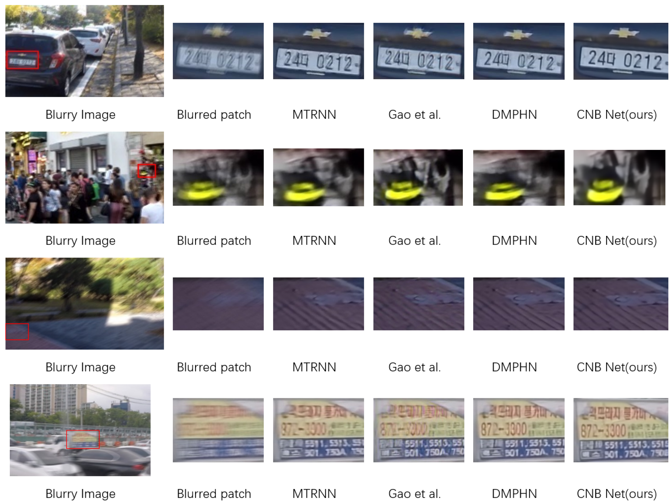
• We perform some experiments on the GoPro dataset and the HIDE dataset and the results are good. We analyze one of the many test samples and plot its features to compare our modules.

2. Related Work

The rapid progress in deep learning, particularly in Convolutional Neural Networks (CNNs), has markedly enhanced the effectiveness of image deblurring, a critical task in areas like handheld photography and security surveillance.

Initial methods primarily addressed static blur, but contemporary CNN models have advanced to adeptly handle dynamic blur scenarios. Despite the diversity in their structures, these models achieve commendable results [1]. For example, Kim et al.’s [8] method employs a sophisticated multi-stage configuration, adept at handling blurs across various scales. This method not only streamlines the flow and integration of multi-scale information but also innovatively integrates a pixel-shuffling mechanism, significantly improving the handling of diverse blurring situations.

Zhang et al. [2] introduce a single-stage image motion deblurring method, effectively extracting local features but somewhat lacking in global context processing. Their approach, utilizing a residual module, a cascade cross-attention module, and a two-scale discriminator module, enhances detail processing. Lian et al. [3] employ a U-Net-based [4] method incorporating attention mechanisms and depth-wise separable convolutions, focusing mainly on local details. Cui et al. [5] propose a novel dual-domain attention mechanism, combining spatial and frequency attention modules, thus addressing both local and frequency-dependent aspects of images. Kupyn et al. [9] develop the Deblur GAN, a GAN-based real-time deblurring method that excels in direct learning from blurred images, efficiently reconstructing missing details. Ali et al.’s [10] survey on Vision Transformers (ViTs) in image restoration tasks points out their prowess in capturing fine details, though they may fall short in processing global context. Ding et al. [11] employ a Transmission-aware network for image restoration, focusing on detail capture but lacking in global scene understanding, especially when handling the Transmission Dark Channel Prior (TDCP), which neglects overall image integrity. Zhang et al. [12] enhance detail extraction via techniques like the Hypercomplex Infrared Fourier Transform (HIFT), focusing on intricate aspects of infrared imagery, but falling short in global scene context processing.

To overcome these limitations, we introduce CNB Net. This model unites convolutional layers with a $5\times 5$ kernel size, normalization, the TSFF module, and the FAS module. It significantly boosts the model’s ability to capture global information while effectively amalgamating it with local details, leading to superior image deblurring quality. Tests on the GoPro and HIDE datasets validate that CNB Net surpasses existing methods across various evaluation metrics.

3. Approach

Traditional deep CNNs often struggle with capturing global information due to their limited receptive fields, as highlighted by Chen et al. [13]. To address this, some researchers, like Lian et al. [3], recommend using convolution with a larger receptive field for better global information comprehension, thereby enhancing deblurring effectiveness. Additionally, attention mechanisms, as proposed by Cui et al. 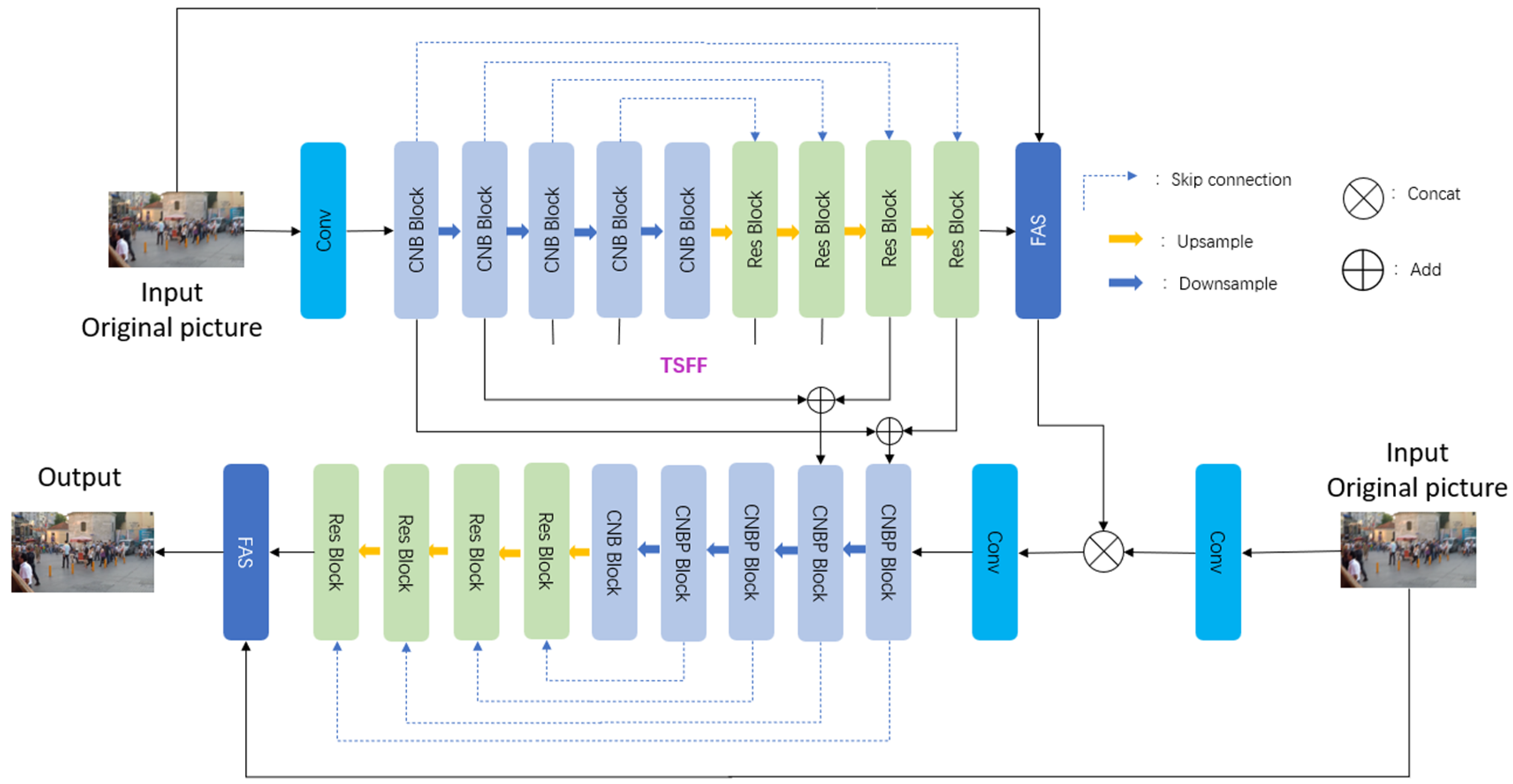[5], have been integrated to more precisely focus on critical image areas for detailed information capture. In light of the complexity of image deblurring and reconstruction tasks, we have designed a novel two-stage architecture named CNB Net, illustrated in Figure 1.

The CNB Net adopts a progressive learning approach in its two-stage architecture. The first stage primarily concentrates on global information extraction and coarse feature learning, aiming to reduce the blur significantly and restore the overall structure and main features of the image. The FAS module, employed at the end of the first stage, helps in extracting local information. The second stage enhances feature extraction by combining local information from the FAS module with multi-scale features from the first stage, using the TSFF module. This stage further processes the image to recover finer details and reduce artifacts like over-smoothing or edge distortions. Our two-stage approach ensures a thorough extraction of global information and detailed capture of specific image details.

Specifically, each stage of CNB Net consists of a sub-network with U-Net [4] as its backbone. Each stage commences with a convolution with a kernel size of $5\times 5$ to extract initial features, which are subsequently fed into an encoder–decoder structure comprising four levels of downsampling and upsampling. Excessive downsampling results in a significant loss of detail, whereas insufficient downsampling may cause the neural network to assimilate an abundance of superfluous information. We use convolution with a kernel size of $5\times 5$ because the dataset involves motion blur caused by camera shake and the motion of the object. In addition, we conducted experiments using different convolution kernels to prove that convolution with a kernel size of $5\times 5$ achieves the best results.

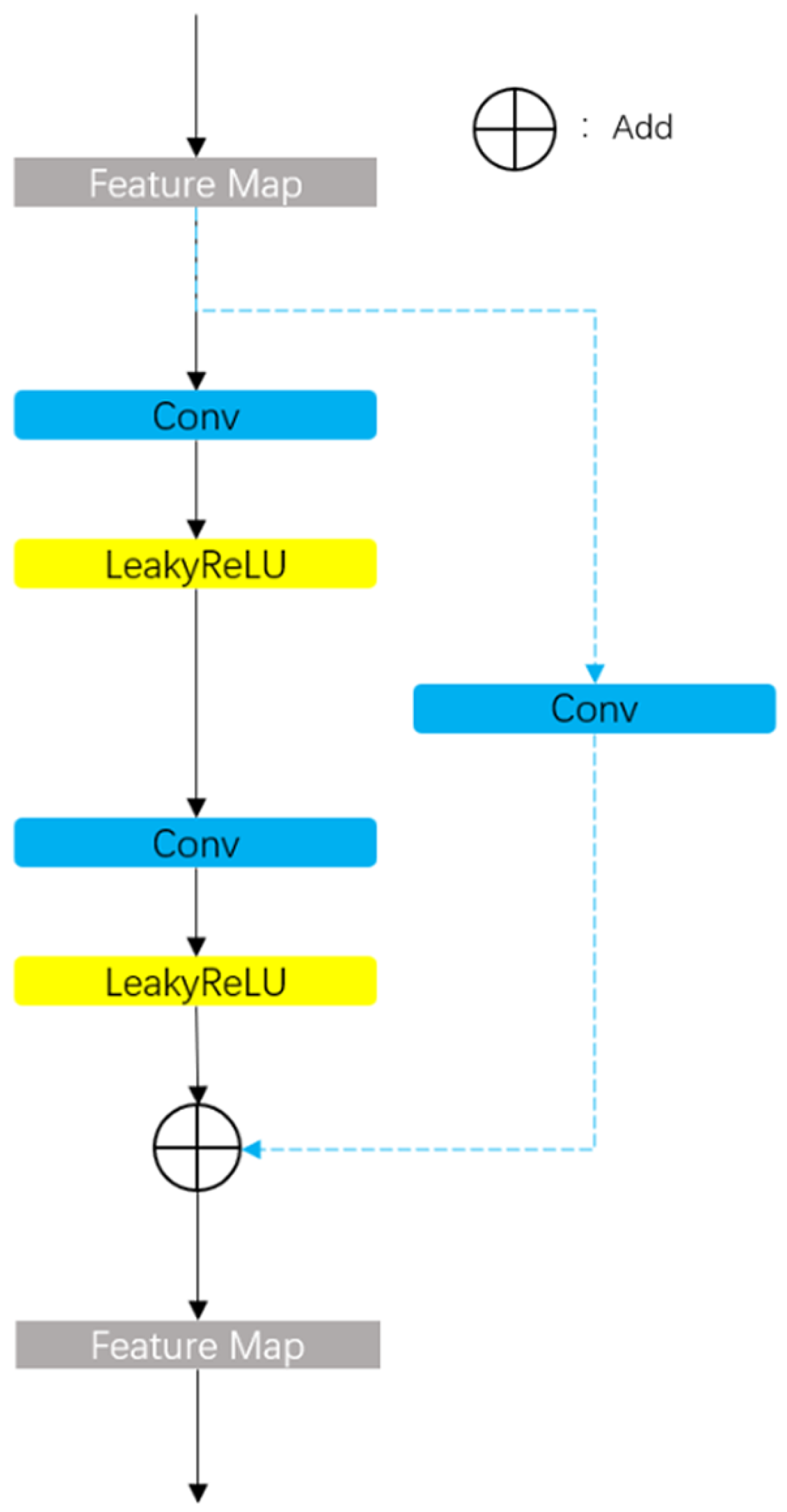
In the encoder component, we design the CNB Block and the CNBP Block to extract features at every scale by doubling the feature channels during downsampling. The detailed introduction of the CNB Block and the CNBP Block is shown in Section 3.1. Within the decoder component, Res Blocks are utilized to capture high-level features and merge them with features from the encoder component via skip connections to compensate for information loss caused by resampling. Figure 2 shows the details of the Res Block. The output image at the end of each stage undergoes processing via the FAS module.

To establish connectivity between the two stages, we use both the TSFF and the FAS modules. In the TSFF module, we leverage convolution with a kernel size of $3\times 3$ to transfer features from the first stage to the second stage while aggregating them alongside second-stage features, thereby enriching multi-scale characteristics within this latter phase. By introducing the FAS module, the network shifts towards detail-oriented information extraction in the second stage specifically. With the FAS module, valuable features from the first stage are actively selected and propagated into the second stage while less informative ones are masked out.

3.1. CNB Block and CNBP Block

The CNB Block and the CNBP Block play a pivotal role in our research endeavors, primarily focused on the effective extraction and processing of multi-scale image features. With the aid of these modules, the CNB Net can extract and process information at various levels within an image.

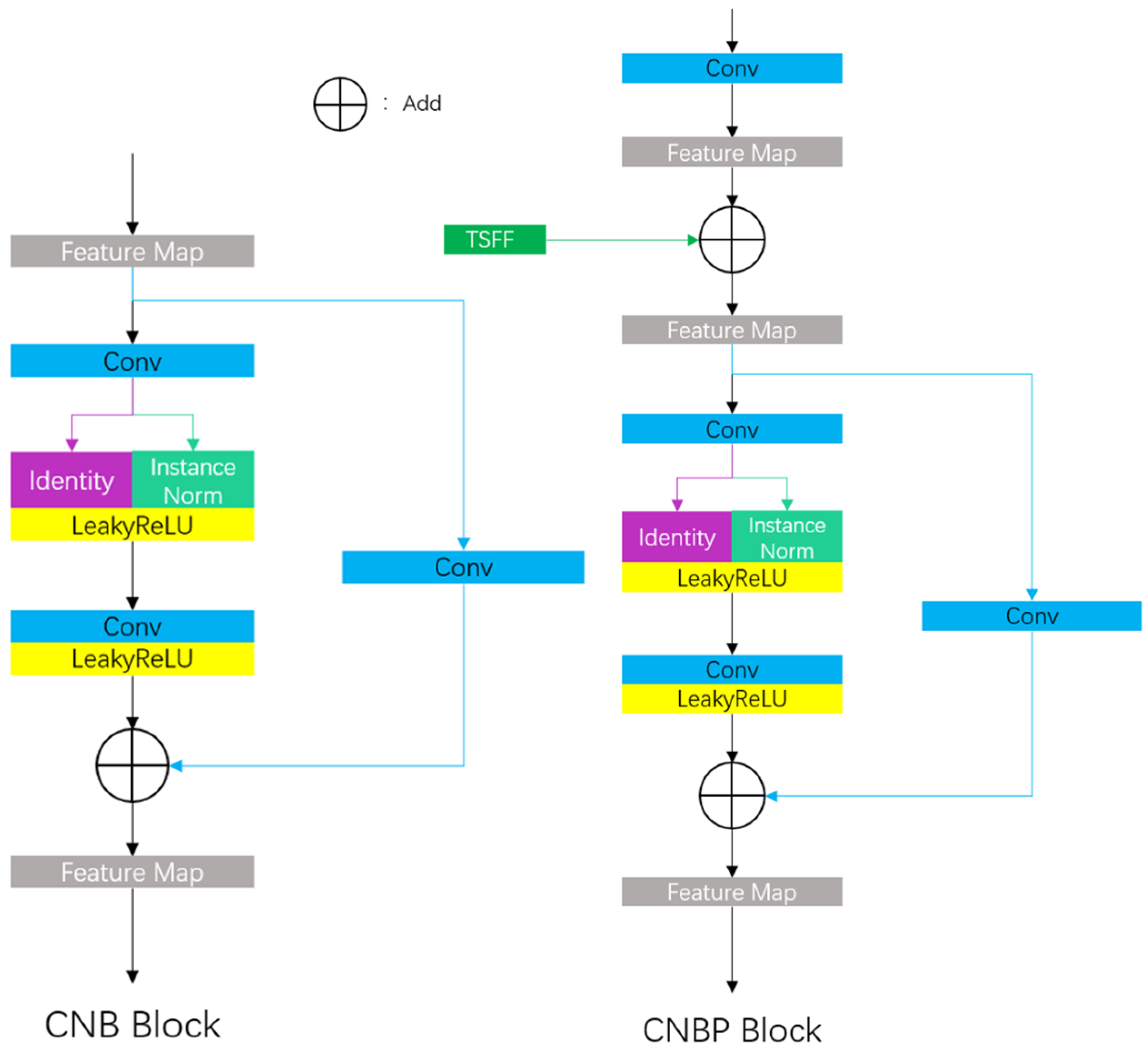
The CNB Block and the CNBP Block employ a distinctive strategy to address the challenges of feature normalization and modeling within convolutional neural networks. The structures of the CNB Block and the CNBP Block are depicted in Figure 3. The initial part of the model consists of a convolutional layer with a kernel size of $5\times 5$, which effectively captures global information from the image, rather than concentrating solely on details such as edges, textures, and shapes. This broad perceptual capability significantly contributes to a comprehensive understanding of the image’s structure and content.

Following the feature extraction by the convolutional layer, an identity mapping and normalization layer are introduced. The identity (ID) mapping component plays a critical role in preserving the original information and features, thereby facilitating effective training of deep networks. The normalization layer is utilized to standardize feature distribution, leading to expedited training processes and improved model generalization. Available normalization methods include Batch Normalization (BN) and Instance Normalization (IN). Based on extensive experimental results, optimal outcomes are achieved by combining ID with IN when training on the GoPro and HIDE datasets, with each method accounting for half of this combination. This unique processing approach enables the CNB Block to perform feature normalization while simultaneously focusing on both local details, such as edges and textures, and preserving global information. Consequently, it attains comprehensive perception of both global and local information. The application of instance normalization assists the model in adjusting feature distribution at the individual sample level, thereby enhancing its generalization ability across different datasets.

Specifically, the CNB Block processes the input feature $F_{\mathrm{in}}\in {\mathbb{R}}^{C_{\mathrm{in}}\times H\times W}$, generating intermediate features $F_{\mathrm{mid}}\in {\mathbb{R}}^{C_{\mathrm{out}}\times H\times W}$ via a convolution layer, where $C_{\mathrm{in}}$ and $C_{\mathrm{out}}$ represent the number of input and output channels, respectively. After generating the intermediate feature $F_{\mathrm{mid}}$, it is divided into two equal parts, $F_{\mathrm{mid}1}$ and $F_{\mathrm{mid}2}$, with $F_{\mathrm{mid}1}=F_{\mathrm{mid}2}=\frac{1}{2}{C}_{\mathrm{out}}$. This division is performed using the torch.chunk function in PyTorch along the channel, and the dimension is 1. Next, the CNB Block applies IN to $F_{\mathrm{mid}1}$, while $F_{\mathrm{mid}2}$ retains the original features via ID, preserving global information from the input features, which aids in providing a more comprehensive feature representation. Subsequently, the instance-normalized feature $F_{\mathrm{mid}1}$ and the identity feature $F_{\mathrm{mid}2}$ are concatenated, resulting in $F_{\mathrm{mid}}=F_{\mathrm{mid}1}+F_{\mathrm{mid}2}$. This combined feature is then passed through a Leaky ReLU activation function with a parameter set to 0.2 followed by a convolution layer with a kernel size of $3\times 3$ and another same Leaky ReLU activation function. Finally, by adding processed features to shortcut features out generated via a convolution layer with a kernel size of $1\times 1$, we obtain the output of the CNB Block denoted as $R_{\mathrm{out}}$.

In the CNB Block and the CNBP Block, the ID branch retains the original information, while the IN branch normalizes the features. Since IN calculates independently for each sample, this is especially useful when dealing with data where the distribution of features varies significantly from batch to batch. For the deblurring task, the feature distribution varies greatly from batch to batch, and choosing IN enables the network to learn complex patterns more effectively. This design aims to further extract and process features introducing non-linearity for enhancing the model’s expressive power, enabling accurate identification and restoration of image details and textures while maintaining gradient stability.

The CNBP Block is a variant of the CNB Block, incorporating an additional connection structure with the TSFF module. By concatenating the output of the TSFF module with the input of the CNB Block, the CNBP Block integrates cross-stage feature information, enabling accommodation of features from multiple stages and achieving synergy between global and local information.

3.2. FAS Module

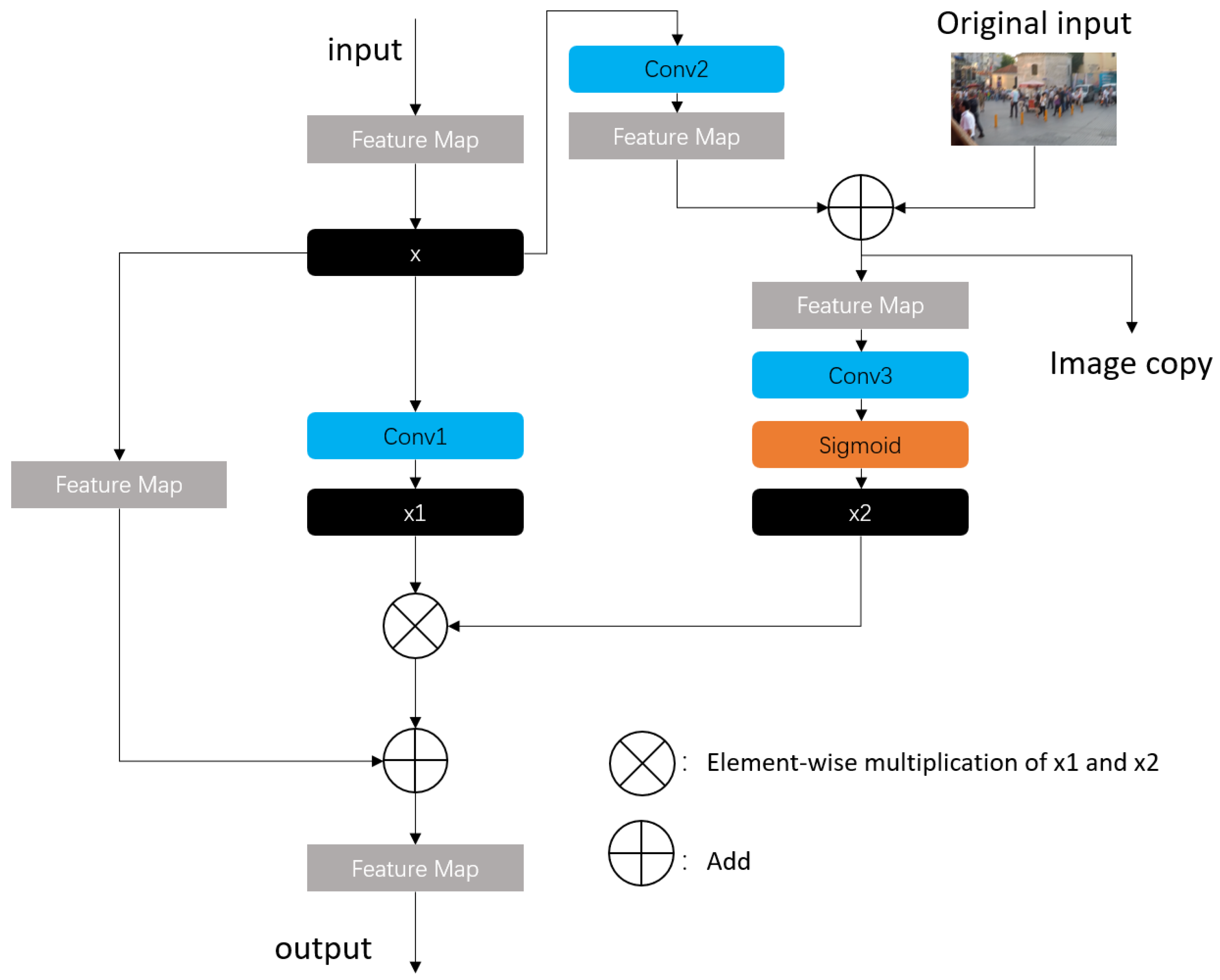
To enhance the perception of local information within the CNB Net architecture, we introduce the FAS module. In the FAS module, $3\times 3$ convolution kernels are utilized, along with bias added to each convolution operation, to boost the model’s learning capability. The structure of the FAS module is shown in Figure 4.

The FAS module initially processes the input feature x through a convolution layer called conv1, generating a feature map $x_1$. It further processes this input feature through another convolution layer called conv2, while combining it with additional image information and the original input. This process generates a modified image represented as an image copy in the diagram. This step aids in focusing on more important regions within input features, such as key objects or salient areas of the image.

Subsequently, the image copy undergoes processing using a third convolution layer called conv3, resulting in the generation of a feature map $x_2$ via the sigmoid function. The feature map $x_2$ ranges between 0 and 1, actively allocating different weights to various spatial locations, thereby highlighting important feature regions while suppressing less significant ones.

By element-wise multiplication of $x_1$ and $x_2$, the FAS module effectively recalibrates the original features, ensuring the network’s focus is concentrated on the most critical features. Finally, the actively selected feature $x_1$ is added to the original input x to retain the original information and further enhance the feature representation.

This design allows the FAS module to not only capture local details in the image, such as edges and textures, but also comprehensively understand and enhance the structure and content of the entire image by actively adjusting spatial attention.

A key function of the FAS module is its ability to process information-rich features at the current stage, streamlining the network’s focus. Those less informative features are masked by using sigmoid function. This functionality is vital in the deblurring process, ensuring both the efficiency and precision of the task at hand.

The FAS module’s active selection mechanism plays a critical role in the network’s performance, directing the net to notice the most pertinent information before progressing to subsequent stages. Implemented at the end of the first stage, the FAS module aids the network in attaining a deeper understanding of the image content, particularly when addressing specific tasks. This fine tuning of feature representation is instrumental for achieving more detailed and higher-quality image restoration in the later stages of the process.

3.3. Loss Function

In the selection of the loss function, we adopt PSNR as the evaluation metric. The PSNR loss function is directly related to the assessment of image quality, where a higher PSNR typically indicates lower distortion. Here, let $S_i\in {\mathbb{R}}^{B\times C\times H\times W}$ denote the input of subnet i, where B is the batch size, C is the number of channels, and H and W represent the spatial dimensions. Similarly, $Y_i\in {\mathbb{R}}^{B\times C\times H\times W}$ represents the output of subnet i, while $G_i\in {\mathbb{R}}^{B\times C\times H\times W}$ represents the ground-truth image for each stage. Then, we optimize the CNB Net end-to-end using Formula (1).

$$\mathrm{LOSS}=-\sum _{i=1}^2\mathrm{PSNR}((S_i+Y_i),G)$$

(1)

To optimize the CNB Net for enhancing performance in image deblurring tasks, we employ the backpropagation algorithm in conjunction with gradient descent methods. This approach is strategically focused on minimizing the PSNR loss. Through this training regimen, the network is conditioned to refine its ability to produce outputs that are increasingly congruent with real images at the pixel level. The primary goal is to systematically diminish the disparity between the predicted image and the ground truth image at each stage of the subnet. By iteratively adjusting the network parameters in this manner, CNB Net is expected to demonstrate marked improvements in image deblurring, ultimately leading to clearer and more accurate image restorations.

4. Experiments

In our image restoration experiments, the PSNR and SSIM are employed as the primary metric for evaluating the quality of the restored images. The datasets leveraged for training, alongside the specific experimental methodologies, are comprehensively detailed in subsequent sections.

4.1. Implementation Details

The training of our model was conducted on the GoPro dataset and the HIDE dataset. The GoPro dataset and the HIDE dataset are publicly accessible resources specifically curated for deblurring tasks.

The GoPro dataset encompasses a total of 2103 image pairs for training purposes, alongside 1111 pairs designated for testing. A noteworthy characteristic of the GoPro dataset is the method employed to generate blurred images: they are created by averaging multiple sharp images captured using a high-speed camera.

The HIDE dataset encompasses a total of 6397 image pairs for training purposes, alongside 2025 pairs designated for testing. It includes multiple blurs caused by the relative movement between an imaging device and a scene, mainly due to camera shaking and object movement.

Our network is trained using the Adam optimizer with a default learning rate of $2\times {10}^{-4}$, which is reduced to $1\times {10}^{-7}$ using a cosine annealing strategy [9]. The model operates on $256\times 256$ patches with a batch size of 32. The training process involved a total of $4\times {10}^5$ iterations.

4.2. Main Results

The results in

Table 1. The comparison with other state-of-the-art (SOTA) deblurring algorithms on the GoPro dataset; our model is highlighted in bold within the table. The inverse filtering method uses a motion fuzzy kernel with different size.

Method	PSNR	SSIM
Inverse filtering method (45 degree, kernel size 7 × 7)	20.14	0.653
Xu et al. [14]	21.00	0.741
Inverse filtering method (45 degree, kernel size 5 × 5)	22.37	0.751
Hyun et al. [15]	23.64	0.824
Whyte et al. [16]	24.60	0.846
Inverse filtering method (45 degree, kernel size 3 × 3)	25.75	0.850
Gong et al. [17]	26.40	0.863
Liang et al. Method-MPRNet [18]	28.55	0.911
Deblur GAN [9]	28.70	0.858
Nah et al. [6]	29.08	0.914
Zhang et al. [19]	29.19	0.931
Deblur GAN-v2 [9]	29.55	0.934
Liang et al. Method-Restormer [18]	30.00	0.9332
Liang et al. Method-Uformer [18]	30.24	0.9346
SRN [8]	30.26	0.934
Gao et al. [20]	30.90	0.935
DBGAN [21]	31.10	0.942
MT-RNN [22]	31.15	0.945
DMPHN [23]	31.20	0.940
Suin et al. [24]	31.85	0.948
CNB Net (ours)	32.21	0.953

show the deblurring comparisons on the GoPro dataset. And, the results in

Table 2. The comparison with other SOTA deblurring algorithms on the HIDE [7] dataset; our model is highlighted in bold within the table. The inverse filtering method uses a motion fuzzy kernel with different size.

Method	PSNR	SSIM
Inverse filtering method (45 degree, kernel size 7 × 7)	18.95	0.447
Inverse filtering method (45 degree, kernel size 5 × 5)	19.64	0.499
Inverse filtering method (45 degree, kernel size 3 × 3)	20.54	0.598
Liang et al. Method-MPRNet [18]	27.25	0.8847
DeblurGAN-v2 [9]	27.40	0.882
SRN [8]	28.36	0.915
Liang et al. Method-Uformer [18]	28.55	0.9080
Liang et al. Method-Restormer [18]	28.71	0.9116
HAdeblur [7]	28.87	0.903
DMPHN [23]	29.09	0.924
Gao et al. [20]	29.11	0.913
MT-RNN [22]	29.11	0.918
Suin et al. [24]	29.98	0.930
CNB Net (ours)	30.38	0.932

show the deblurring comparisons on the HIDE dataset. We achieve an improvement of 0.36 dB in PSNR and 0.005 in SSIM over the previous best method on the GoPro dataset. And, we achieve an improvement of 0.4 dB in PSNR and 0.002 in SSIM over the previous best method on the HIDE dataset.

4.3. Quality Experiments

In Table 1, we demonstrate the effectiveness and superiority of CNB Net on the GoPro dataset. Additionally, we conduct quality experiments to validate the superiority of our proposed method. We select a subset of models from the models described above for comparison with our model, which is shown in Figure 5.

5. Discussion

5.1. Parameter Setting

The core idea of CNB Net revolves around the CNB Block. In this section, we conduct several experiments to evaluate the CNB Block from various perspectives. First, we evaluate the CNB Block in terms of multiply–accumulate operations (MACs). MACs, as an evaluation metric, measures the total number of multiplications and additions required for the model to perform one forward propagation. This metric is independent of the specific content of the input data, only related to the architecture of the model (e.g., number of layers, size, stride, etc.) and the shape of the input data. We evaluate the MACs using a random input to the model, which incorporates different normalization methods. The input is a random tensor with $256\times 256$ pixels and RGB channels.

Table 3. Comparison of different normalization methods on the GoPro dataset with ID, BN, and IN.The method $\frac{1}{2}$ ID and $\frac{1}{2}$ IN yields the best results. The best results are shown in bold.

Method	PSNR	SSIM	MACs
1 ID	31.11	0.942	192.39G
1 IN	31.92	0.950	192.42G
1 BN	31.26	0.940	192.42G
$\frac{1}{2}$ ID and $\frac{1}{2}$ BN	31.34	0.941	192.41G
$\frac{1}{2}$ ID and $\frac{1}{2}$ IN	32.21	0.953	192.41G
$\frac{1}{2}$ BN and $\frac{1}{2}$ IN	31.41	0.946	192.41G

shows the results with different normalization methods.

The values in the table are represented in italicized bold for the lowest values and underlined for the highest values. It can be observed that using a combination of $\frac{1}{2}$ ID and $\frac{1}{2}$ IN yields the best results. This approach not only improves accuracy but also slightly reduces the parameter count.

All the experimental results presented below utilize the FAS module and the TSFF module. For the normalization part of the CNB Block, a combination of $\frac{1}{2}$ ID and $\frac{1}{2}$ IN is employed, as shown in Figure 6 and

Table 4. Comparison of PSNR and SSIM for different receptive field sizes in the convolutional layers of CNB Net with $\frac{1}{2}$ ID and $\frac{1}{2}$ IN on the HIDE dataset. The best results are shown in bold.

Kernel Size	PSNR	SSIM
3 × 3	29.97	0.928
5 × 5	30.38	0.932
7 × 7	29.14	0.921

.

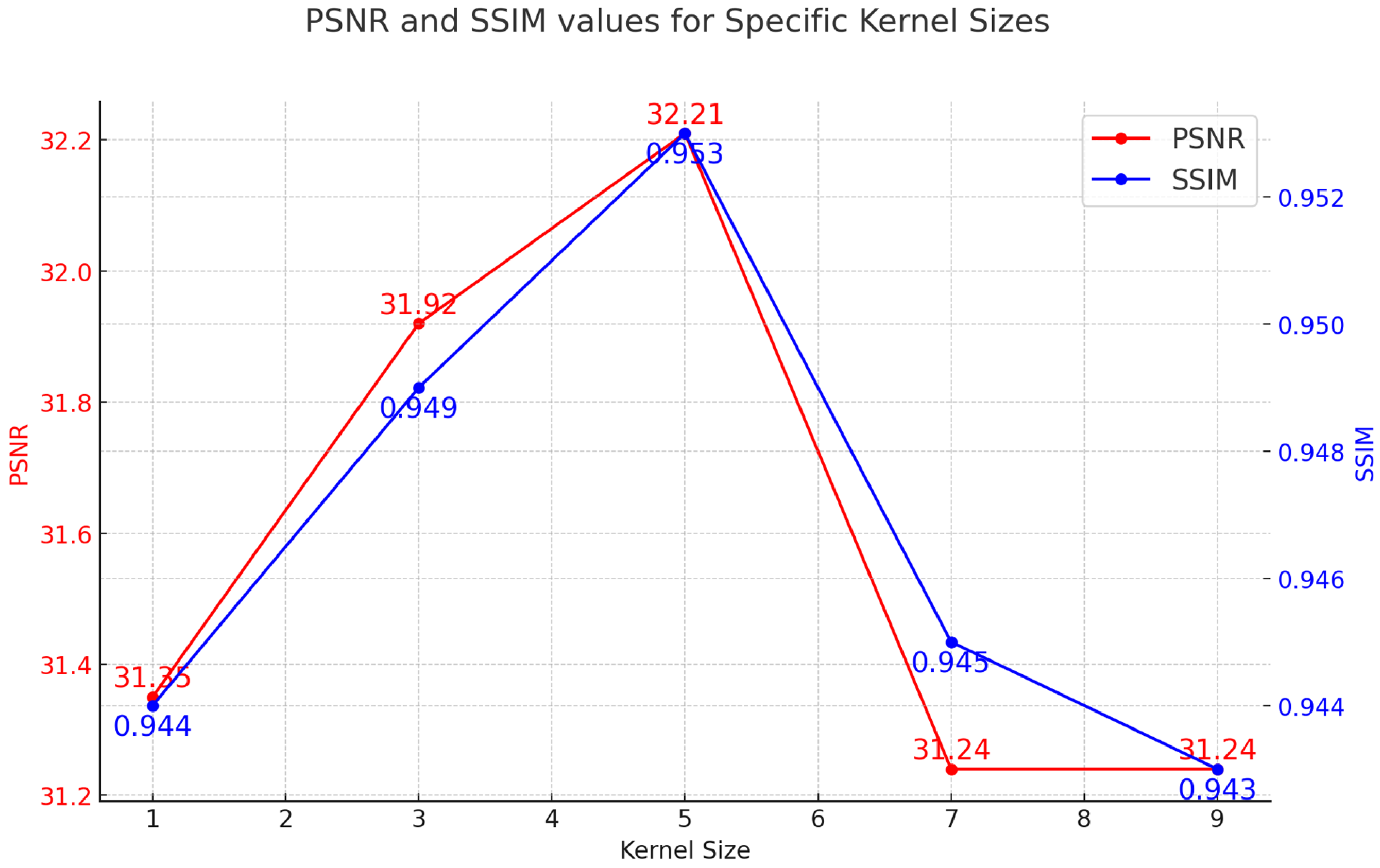
In our experiment, on the GoPro dataset, the use of convolution with a kernel size of $5\times 5$ resulted in a PSNR of 32.2 and a SSIM of 0.953, which is the best outcome among all of the configurations we tested. And, on the HIDE dataset, the use of a $5\times 5$ receptive field convolutional kernel resulted in a PSNR of 30.38 and a SSIM of 0.932.

In contrast, kernels with receptive fields smaller than $5\times 5$ were unable to capture global information, adversely affecting the overall performance of the model. Additionally, the convolution kernels larger than $5\times 5$, due to their excessively large receptive fields, led to a loss of detail and also negatively impacted the model’s overall performance.

Although, $3\times 3$ convolutional kernels are often favored in certain scenarios due to their smaller parameter count and computational efficiency. In our experiments, the 5 × 5 convolution kernels have larger receptive fields than $3\times 3$ convolution kernels and are more effective in feature extraction, thereby enhancing the accuracy of the model.

5.2. Ablation Experiments

We conduct numerous experiments where we consider the approach that uses the Identity method as the baseline, and the results comparing different receptive field sizes with various normalization methods are presented in

Table 5. Comparison of PSNR and SSIM for different receptive field sizes in the convolutional layers of CNB Net with different normalization method on the GoPro dataset. The best results are shown in bold.

Kernel Size	ID	BN	IN	PSNR	SSIM
5 × 5	1	-	-	31.11	0.942	(baseline)
5 × 5	-	1	-	31.26	0.940
5 × 5	-	-	1	31.93	0.950
3 × 3	1	-	-	30.98	0.941	(baseline)
3 × 3	-	1	-	31.15	0.940
3 × 3	-	-	1	31.76	0.948

,

Table 6. Comparison of PSNR and SSIM for different receptive field sizes in the convolutional layers of CNB Net, employing various normalization methods on the GoPro dataset. The network architecture incorporates a two-part feature segmentation strategy, where each segment undergoes distinct normalization before being recombined. The best results are shown in bold.

Kernel Size	ID	BN	IN	PSNR	SSIM
5 × 5	-	1	1	31.41	0.946
5 × 5	1	1	-	31.34	0.941
5 × 5	1	-	1	32.21	0.953
3 × 3	-	1	1	31.27	0.945
3 × 3	1	1	-	31.28	0.940
3 × 3	1	-	1	31.92	0.950

and

Table 7. Comparison of PSNR and SSIM for different receptive field sizes in the convolutional layers of CNB Net, employing various normalization methods on the GoPro dataset. The network architecture incorporates a four-part feature segmentation strategy, where each segment undergoes distinct normalization before being recombined. The best results are shown in bold.

Kernel Size	ID	BN	IN	PSNR	SSIM
5 × 5	1	-	3	31.92	0.949
5 × 5	1	1	2	31.26	0.943
5 × 5	1	2	1	31.26	0.942
5 × 5	1	3	-	31.05	0.939
5 × 5	2	1	1	31.28	0.945
5 × 5	3	1	-	31.28	0.942
5 × 5	3	-	1	31.32	0.944
3 × 3	1	-	3	31.62	0.948
3 × 3	1	1	2	31.23	0.943
3 × 3	1	2	1	31.24	0.942
3 × 3	1	3	-	31.31	0.941
3 × 3	2	1	1	31.16	0.944
3 × 3	3	1	-	31.11	0.941
3 × 3	3	-	1	31.20	0.942

.

Using 5 × 5 convolution kernels to extract features gives better results than 3 × 3 convolution kernels. Regarding the phenomenon where IN yields better results compared to BN in the provided data, we conduct an analysis.

To illustrate, BN aims to address the issue of covariate shift in deep learning. It ensures that the outputs of each layer in a deep network have consistent means and standard deviations across the entire dataset. During training, as these statistics are unconstrained and can vary randomly, this can lead to numerical stability issues. BN reduces this uncertainty by normalizing the layer outputs. However, due to the computational cost of calculating the mean and standard deviation over the entire dataset, these calculations are performed only on each batch of data. This approach has its limitations: if the batch statistics significantly differ from the overall dataset, it may lead to performance degradation. To obtain more stable statistics, sometimes additional forward passes need to be performed during training.

Formula (2) is used for normalizing the input features. Formulas (3) and (4) are used to calculate the mean and standard deviation of N elements in batch i, respectively. Formulas (5) and (6) are the update formulas for the mean and standard deviation, respectively, where $1-ϵ$ represents the momentum (or persistence) of previous samples.

$$\begin{array}{cc}\hfill \widehat{{\mathbf{X}}_i}& \hfill =\frac{{\mathbf{X}}_i-{\mathbf{m}}_i}{{\mathbf{œ}}_i}\hfill \end{array}$$

(2)

$$\begin{array}{cc}\hfill {\mathbf{m}}_i& \hfill =\frac{1}{N}\sum {\mathbf{X}}_k\hfill \end{array}$$

(3)

$$\begin{array}{cc}\hfill {\mathbf{œ}}_i^2& \hfill =\frac{1}{N}\sum {\mathbf{X}}_k^2-{\mathbf{m}}_i^2\hfill \end{array}$$

(4)

$$\begin{array}{cc}\hfill \widehat{{\mathbf{m}}_{t+1}}& \hfill =(1-ϵ)\widehat{{\mathbf{m}}_t}+ϵ{\mathbf{m}}_t\hfill \end{array}$$

(5)

$$\begin{array}{cc}\hfill \widehat{{\mathbf{œ}}_{t+1}}& \hfill =(1-ϵ)\widehat{{\mathbf{œ}}_t}+ϵ{\mathbf{œ}}_t\hfill \end{array}$$

(6)

While BN reduces covariate shift by adjusting the unit values for each batch, it may introduce noise due to the randomness of training batches. Furthermore, in deblurring tasks, small variations in features are crucial. BN can diminish these subtle feature differences via normalization. This can result in reduced sensitivity of the model to important features. Unlike BN, IN normalizes each individual data instance (such as a single image) independently. This means it is not affected by batch size or variations between batches, making the model more stable, especially when dealing with images that have varying sizes, styles, or content. IN exhibits a higher adaptability to changes in input data due to its independent processing of each instance. This is particularly important when dealing with image datasets that exhibit high variability.

5.3. Evaluation of FAS Module and TSFF Module

In addition to the evaluation of the CNB Block module, we also conducted ablation experiments to assess the impact of using the FAS module and the TSFF module. In the case of using $\frac{1}{2}$ ID and $\frac{1}{2}$ IN with 5 × 5 convolutional kernels, we conduct two separate comparisons: firstly, comparing the PSNR and SSIM with and without the TSFF module in the presence of the FAS module; secondly, comparing the PSNR and SSIM with and without the FAS module when the TSFF module is present. The results are shown in

Table 8. Comparison of PSNR and SSIM with and without the use of the FAS and TSFF modules on the GoPro dataset. The presence of a ‘✓’ symbol indicates the inclusion of a particular module within the model, whereas the symbol ’×’ denotes the absence of such a module.

FAS Module	TSFF Module	PSNR	SSIM
×	×	30.10	0.933	(baseline)
×	✓	31.22	0.940
✓	×	31.24	0.942
✓	✓	32.21	0.953

.

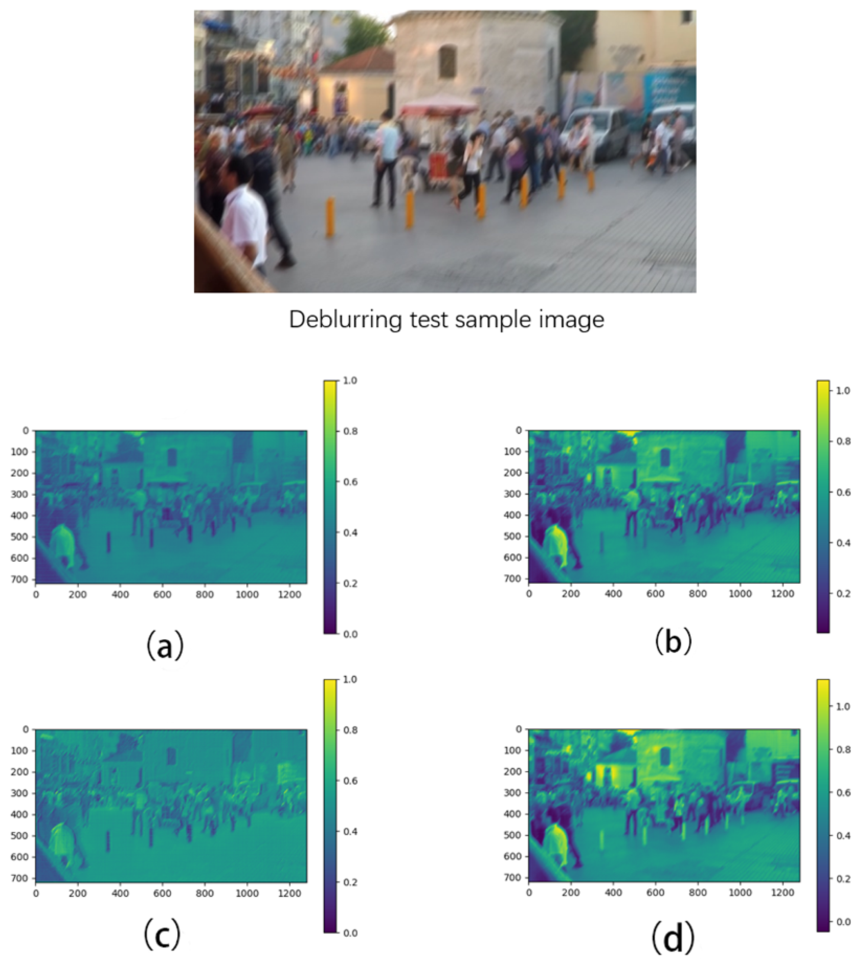
Our experiments demonstrate that the incorporation of the FAS module and the TSFF module notably enhances the accuracy in image restoration tasks. We conduct tests for both the FAS module and the TSFF module, and we select one test sample from among numerous test cases. 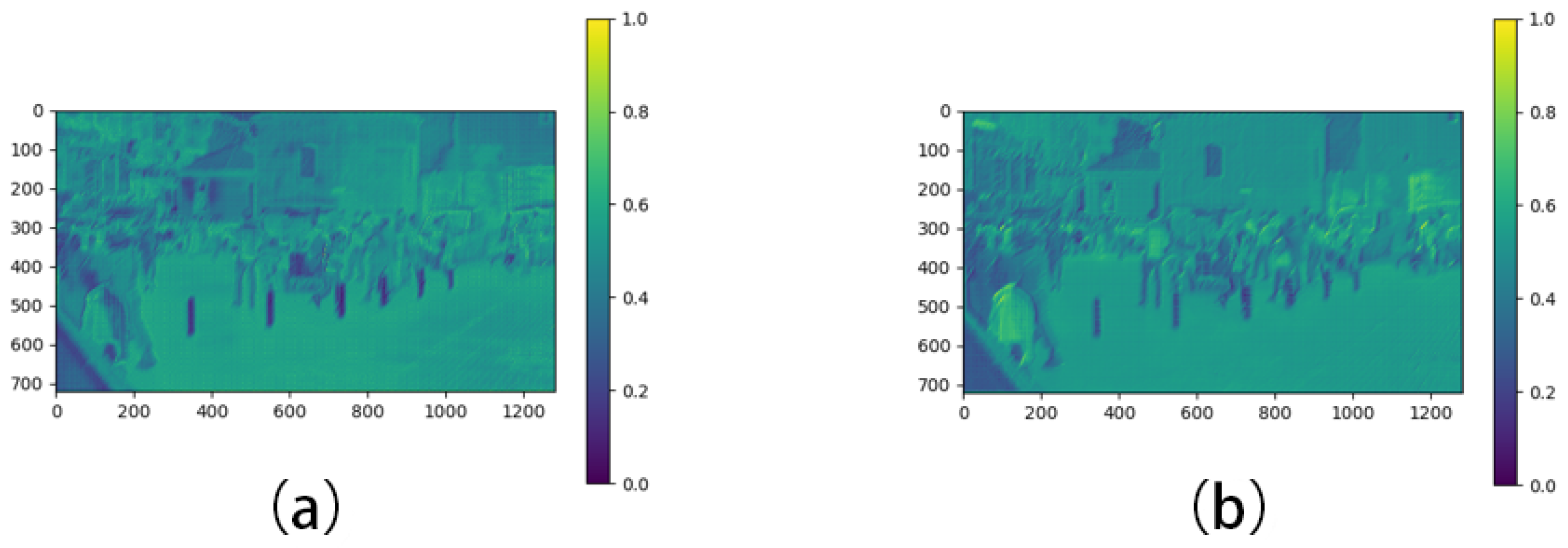In the case of using $\frac{1}{2}$ ID and $\frac{1}{2}$ IN with 5 × 5 convolutional kernels, Figure 7 shows the comparisons of the FAS module in different stages and Figure 8 shows the comparison with or without the TSFF module.

For the FAS module, we extract feature maps that have passed through this module and those that have not, then perform visualizations on them. For the TSFF module, we extract feature maps with this module and without this module, then perform visualizations on them.

For the visualization part, we generate average feature maps from the test samples across the RGB channel. We utilize the Viridis color mapping from the PLT package and normalize the values to the range of zero to one. In this mapping, zero corresponds to deep blue, while one corresponds to yellow–green. Areas on the image close to one will appear as bright yellow or yellow–green, indicating high activation strength in those regions. Conversely, regions close to zero will appear as dark blue, signifying low activation strength. These bright areas represent the portions of the image that the network deems highly important for the task, while the dark areas indicate the opposite.

After feature map extraction, we observe that the activation distribution becomes more concentrated, and the activation intensity increases when passing through the FAS module compared to not using it. This suggests that certain regions in the feature map become noticeably darker or brighter than others when employing the FAS module, indicating that the features extracted with the FAS module are more detailed and focused. The FAS module plays a pivotal role in the entire deblurring process.

Similarly, to assess the impact of the TSFF module, we conduct feature map extractions both with and without it, focusing specifically on the second stage before involving the FAS module. This comparative analysis provides insights into the distinct enhancements brought about by the TSFF module in the multi-scale feature representation process, further substantiating its crucial role in our deblurring methodology.

After extracting the feature maps, we observe that with the TSFF module, the activation intensity is stronger and the smoothness is higher compared to when it is not present.

6. Limitations and Future Work

In this study, we aim to develop a more effective method for image deblurring. Although deep learning-based approaches have shown significant advancements in enhancing visual quality, there is still potential for improvement. Various factors can influence the model’s performance, as noted by Zhang et al. [1]. For instance, our current loss function relies solely on the PSNR metric. Moving forward, we plan to integrate both PSNR and SSIM metrics into our loss function to investigate their impact on model performance. Additionally, we intend to experiment with other loss functions, such as the frequency-domain approach suggested by Yadav et al. [25].

Introducing supplementary information has been proven to enhance performance in many tasks [26]. In our research, we have found that using the ’Segment Anything’ annotation method [27] helps in obtaining images with clearly defined objects. This provides the network with more explicit structural information, offering additional support to the deblurring algorithm. Such segmentation aids the model in more accurately localizing and addressing blurred areas.

7. Conclusions

In this study, we develop the CNB Block, which represents an innovative approach by integrating large receptive fields with advanced normalization techniques. This novel combination enhances our ability to capture and process complex image features effectively. Expanding upon the foundation of the CNB Block, we have introduced a two-stage network structure named CNB Net. This architecture incorporates the TSFF module to facilitate a two-stage feature flow, thereby significantly improving our ability to represent multi-scale features accurately. Furthermore, we have introduced the FAS module, which plays a pivotal role in enabling active feature selection and propagation to the subsequent stage of the network. As a result of these advancements, images reconstructed and restored using our proposed method have demonstrated superior quality compared to existing techniques.