1. Introduction
Mariculture, as an industry with a long history in China, has important economic and ecological benefits [
1,
2]. Water quality is an important factor that cannot be ignored by farmers, and the content of nitrite is a key indicator for evaluating the quality of mariculture water [
3]. Nitrite is toxic to aquatic species; it can change the deoxyhemoglobin in the blood into methemoglobin, thus further affecting the ability of blood to carry oxygen [
4]. Therefore, the nitrite content in water cannot be higher than the maximum concentration that aquatic organisms can withstand, otherwise there will be an outbreak of illness or death. It is very necessary to master the nitrite content in the water in real time for the water quality management of mariculture. Most of China’s fisheries are small-scale domestic aquaculture, and aquaculture personnel often judge the nitrite content in the water based on their life experience (they roughly observe water bodies, such as whether the water bodies have become turbid or whether aquatic organisms have abnormal or died); this experiential method of water quality detection often leads to the deterioration of water quality due to judgment errors, resulting in economic losses.
At present, there are two main accurate methods for detecting nitrite content in water environments. One method is spectrophotometry [
5]: The principle of this method is the diazotization of aniline and nitrite in hydrochloric acid medium, and then reaction with hydroxyl of α-Naphthol in NaOH solution to produce orange red azo dyes (the reaction formulas are shown in (1) and (2)); the maximum absorption wavelength of this azo dye is 480 nm. This method utilizes the principle of molecular absorption spectroscopy. When external energy is applied to the molecules of the substance under examination, the substance’s internal constituents will absorb or release energy in the form of electromagnetic radiation. When radiation energy acts on transparent or semitransparent materials to be detected, the material will absorb radiation energy at frequencies corresponding to its state changes and transition to higher energy levels. Therefore, a method for determining nitrite using spectrophotometry has been established.
The second method is chemical colorimetry: The principle of this method is to determine the content of nitrite in the water environment by comparing it with the colorimetric card through the color reaction between nitrite and the detection reagent (the reaction formulas are shown in (1) and (2)). Compared to the former, the latter has lower costs and is more easily accepted by small-scale farmers, but this method also has significant drawbacks, for example, environmental factors such as background color, light intensity, and the sensitivity of the experimenter’s eyes to color when compared with a color comparison card can affect the difficulty, speed, and accuracy of judgment. Spectrophotometry has the advantage of high accuracy and the disadvantage of using a more expensive spectrophotometer. The advantage of the chemical colorimetry method is that it is very low-cost, but its disadvantages are also obvious, such as the dependence on life experience and the higher sensitivity of the human eyes to color.
With the development of computer technology, the application of deep learning [
6] is becoming increasingly widespread, such as autonomous driving, “Smart Healthcare”, earthquake prediction, etc. In addition, currently, deep learning is also applied in the field of aquaculture.
Table 1 shows the different water quality monitoring methods and parameters.
With the emergence of convolutional neural networks such as Alex Net [
15], ZFNet [
16], VGGNet [
17], GoogLeNet [
18,
19,
20], ResNet [
21], the application of image recognition technology based on deep learning is becoming increasingly widespread; it utilizes deep neural networks to automatically extract and learn the features of the input image, thereby achieving tasks such as the classification, detection, and segmentation of image content. The core idea of this technology is to gradually abstract and represent the features of data through multilayer neural network models, thereby enabling better understanding and processing of image data, and it has now been applied in medical image analysis, natural language processing, object detection, object recognition and classification, facial recognition, agriculture and environmental monitoring, and other fields. Therefore, this article applies machine vision to the detection of nitrite content in an aquaculture water environment, and the purpose of this study is to propose a low-cost and high-accuracy nitrite detection method. The innovation of this method lies in utilizing machine vision to replace human eyes for judgment, achieving an effective combination of high recognition accuracy and low-cost detection.
2. Materials and Methods
2.1. Dataset
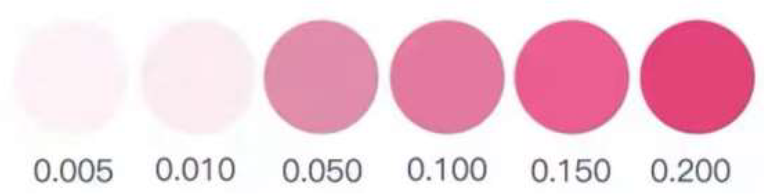
The colorimetric card used in the chemical colorimetric method calibrated nitrite concentrations of 0.005 mg/L, 0.010 mg/L, 0.050 mg/L, 0.100 mg/L, 0.150 mg/L, and 0.200 mg/L (as shown in
Figure 1); therefore, this experiment used sodium nitrite, artificial seawater salt, and distilled water to prepare nitrite water samples, with concentrations ranging from 0.010 mg/L to 0.200 mg/L and gradients of 0.010 mg/L, as well as nitrite water samples with concentrations of 0.005 mg/L. The specific operational processes are as follows:
- (1)
Configure seawater without nitrite: Mix artificial seawater salt (which is already produced by the Bessn brand) and distilled water in a ratio of 1:30 and make the seawater salt to fully dissolve.
- (2)
Add quantitative nitrite: For example, when preparing 0.200 mg/L nitrite water sample, weigh 1.971 g sodium nitrite, prepare 1 L solution, and then dilute it 2000 times to obtain the water sample with the target concentration. The concentration here refers to the concentration of N element, and the proportion of N element in sodium nitrite is 14/69. The same applies to configuring water samples of other concentrations.
Then, 198 images were taken under different lighting intensities (including natural light with different intensities, natural light with different intensities of light sources, and different intensities of light sources in a darkroom). The detailed information of the materials used is shown in
Table 2, and the detailed parameters of the camera used in this experiment are shown in
Table 3.
2.2. Methods
The above methods combine deep learning with spectral-based detection methods, but due to the expensive spectrometer used (for example, the price of Hash’s DR900 portable detector is as high as CNY 21,591), they are difficult for small farmers to accept; therefore, this experiment explores a lower-cost method. This experiment combines deep learning image recognition algorithm with chemical colorimetry, utilizing the advantages of low cost and fast reaction of chemical reagents, as well as the advantages of machine learning. By using machines instead of human eyes to make judgments, it eliminates concerns about judgment errors due to the human eye’s insufficient sensitivity to colors, and also alleviates worries about the impact of ambient light or background on human judgment. The specific procedures of this method are as follows:
- (1)
Collect 15 mL of the water sample to be tested;
- (2)
Sequentially add 5 drops of reagent A and B for testing;
- (3)
Shake the mixture thoroughly and let it settle for 5 min;
- (4)
Capture an image of the water sample using a camera;
- (5)
Use deep learning networks to identify captured photos.
This method can be applied to the detection of nitrite content in the water environment of mariculture; it can quickly and accurately grasp the water quality status, so as to better carry out water quality management work and improve production efficiency. The main advantages and disadvantages of different methods for detecting nitrite content in aquaculture water environment are compared in
Table 4.
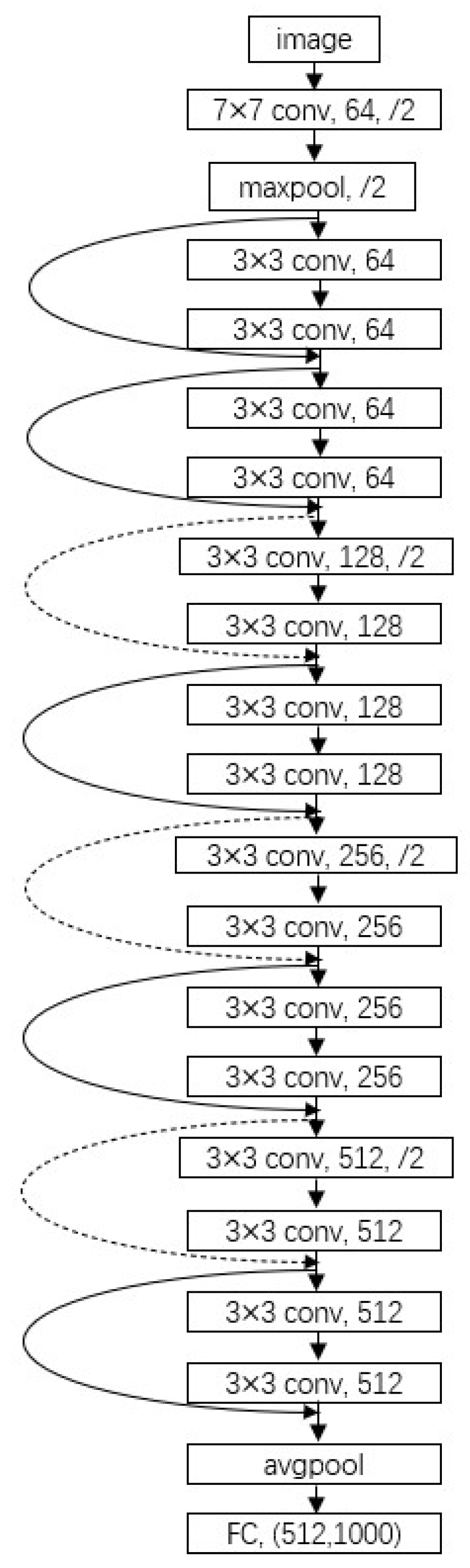
This experiment used ResNet to recognize nitrite water samples after titration, with a network depth of 18 layers, namely ResNet18. The number 18 represents the weight layer of the network, which has a total of 18 layers, including 17 convolutional layers and 1 fully connected layer.
Figure 2 shows the basic network architecture of ResNet18, which includes information such as changes in input image size and the number of network layer channels. The input is a three-channel RGB image, with a size of 224 × 224. The first convolutional layer has 64 convolutional kernels of 7 × 7, with a stride of 2, and the output size is 112 × 112. In the second convolutional layer, apply max pooling using a 3 × 3 convolutional kernel first, and then apply two residual blocks, with each block utilizing 64 convolutional kernels of 3 × 3 and is executed twice. The output size of the second convolutional layer is 56 × 56. In the third convolutional layer, there are two residual blocks, each consisting of 128 convolutional kernels of 3 × 3, and each convolution is performed twice. The output size of the third convolutional layer is 28 × 28. The fourth and fifth convolutional layers both contain two residual blocks, each with a size of 3 × 3, and each convolutional operation is performed twice. The difference is that each residual block in the fourth convolutional layer has 256 convolution kernels, while each residual block in the fifth convolutional layer has 512 convolution kernels. The output sizes of the fourth and fifth convolutional layers are 14 × 14 and 7 × 7, respectively. Finally, an average pooling layer and a fully connected layer are applied, with output dimensions of 512 and 1000, respectively.
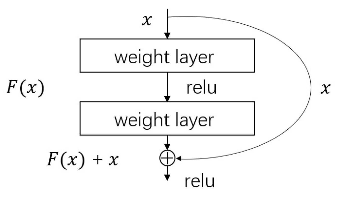
The key module of this network is the residual block, as shown in
Figure 3; it is also the core idea of ResNet. Fit potential mapping
using the sum of residual mapping
and identity mapping
, i.e.,
The identity mapping is called “shortcut”, and the “⊕” is element-wise addition; it requires that the dimensions of
and
participating in the operation must be the same. This structure can solve the problem of network degradation: if, at some point, the network has reached its optimal state and continues to increase the network depth, the residual mapping
will tend to 0, while the identity mapping
remains unchanged. Therefore, the effectiveness of the network remains optimal.
This experiment replaced some residual blocks in the network with the ResNeXt module. The original ResNet-18 contains 4 stages, with each stage containing 2 residual blocks. Now, replace the residual blocks for two of the stages, with the specific design as follows:
- (1)
Stage 1: Use the original 2 residual blocks, unchanged.
- (2)
Stage 2: Replace with 2 ResNeXt blocks. Each ResNeXt block contains 4 branches, each consisting of 64, 1 × 1 convolutional layers and 64, 3 × 3 convolutional layers. The sum of the output numbers of the 4 branches is equal to the number of channels in the original residual block, which is 256.
- (3)
Stage 3: Use the original 2 residual blocks, unchanged.
- (4)
Stage 4: Replace with 2 ResNeXt blocks. Each ResNeXt block contains 4 branches, each consisting of 128, 1 × 1 and 128, 3 × 3 convolutional layers. The sum of the output numbers of the 4 branches equals the number of channels in the original residual block, which is 512.
Through this design, a total of 4 ResNeXt blocks were introduced to replace the residual blocks of Stage 2 and Stage 4, while the remaining stages remained unchanged. This network design has the following benefits:
- (1)
Replacing only a portion of the layers can introduce ResNeXt’s innovation while inheriting the advantages of the original network framework.
- (2)
Utilizing the multibranch structure of the ResNeXt module to extract richer feature representations and enhance the network’s feature expression capabilities.
- (3)
Replace the middle layer segments, which learn features with higher semantic levels. Introducing a multibranch structure is more crucial for improving discriminability.
- (4)
Preserving the original structure of the first and last layer segments can utilize the pretrained weights of these layers to accelerate training convergence.
In the field of deep learning, many parameter adjustment techniques and improvement methods have emerged to improve the effectiveness of the model, and adding attention mechanisms [
22,
23] is a common method among them. It can make the model more flexible in processing input data. For the effective information in the input data, attention mechanism can assign them higher weights, while for those unrelated parts, attention mechanism will assign them lower weights or ignore them; by this way, the performance of the model can be improved. This experiment incorporated SE [
24] and CBAM [
25] into the framework of residual networks.
The SE (squeeze and excitation) attention mechanism is to add attention mechanisms to the channel dimension, and the key operations are squeeze and excitation; the specific steps are as follows:
- (1)
Squeeze: Perform global average pooling on the feature map to generate a vector (with a size of 1 × 1 × C, where C represents the channel), where each channel is represented by a numerical value.
- (2)
Excitation: Perform two full connections on the results obtained by squeeze, followed by sigmoid activation, to obtain a weight matrix.
- (3)
Scale: Add the weight values obtained earlier to the features of each channel.
CBAM (convolutional block attention module) and SE have certain similarities, but the difference is that the former focuses on spatial dimensions as well as channel dimensions, CBAM can be divided into two modules:
- (1)
Channel attention module: This module is similar to SE, but it has an additional global maximum pooling, which means it extracts richer features.
- (2)
Spatial attention module: The feature map obtained from channel attention module serves as the input for this module, and then maximum pooling and average pooling are applied sequentially. Then, a 7 × 7 convolutional kernel is used to further extract features, and finally, the spatial attention weight is obtained through sigmoid activation layer.
2.3. Data Preprocessing
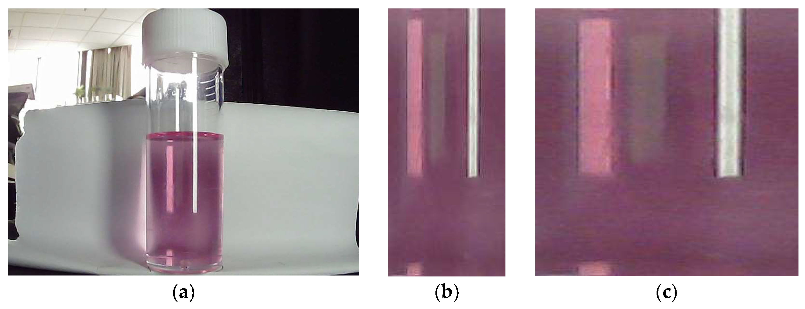
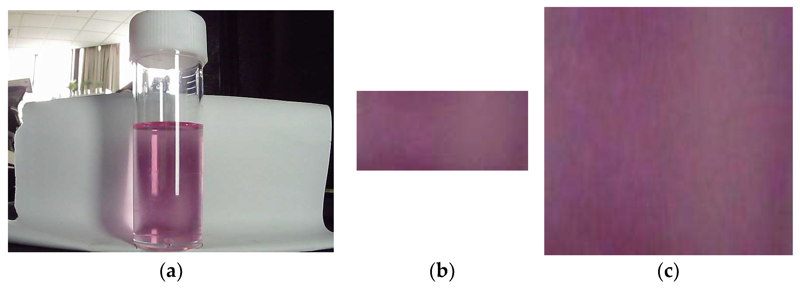
In order to eliminate the influence of irrelevant features such as environmental factors in the photos (such as
Figure 4a), it is necessary to crop the photos and only retain the portion of the test tube containing the water sample (
Figure 4b). This can not only accelerate the training speed of the model, but also improve the accuracy of the results. The resolution of the cropped photo was approximately 105
240. The Pytorch framework used in this experiment requires a three channel RGB image for the pretrained model, and the height and width of the image should be at least 224; therefore, the cropped photo is scaled to 256
256 (
Figure 4c) to facilitate subsequent normalization processing of the dataset.
Before network training, it is necessary to augment the dataset as it can prevent network overfitting. This experiment used rotation, mirroring, and other methods to augment the initial dataset by a factor of six without changing the original color characteristics of the pictures, and the dataset’s size became 1188 images. Then, the dataset was further augmented by using a random cropping method to crop the image size to 224 224 pixels, which means online augmentation. During the model training process, the data were augmented while training. This data augmentation method avoids synthesizing the augmented data without occupying additional storage space. In theory, the amount of data during the training process is much greater than the original data, and each epoch trains different images. It can achieve good results in tasks such as image classification that do not require high data changes.
Next, the data were transformed into a Gaussian distribution, which standardized the images channel by channel (changing the mean of the image to 0 and the standard deviation to 1), making it easier for the model to converge during training, as shown in (3):
In (3), represents the standard deviation of the channel. The mean is the average level of a set of data, while the standard deviation represents the degree of dispersion of the data. The mean and standard deviation of a dataset can effectively summarize the information and features of this set of images.
2.4. Training the Neural Network
First, the preprocessed dataset was divided into four categories: 0.050 mg/L, 0.100 mg/L, 0.150 mg/L, and 0.200 mg/L. Second, they were divided into training set, validation set, and test set according to the ratio of 7:1:2, and then the network parameters such as batch size, epoch, and learning rate were adjusted.
Choosing a good learning rate is crucial to the effectiveness of the network. There are many training techniques for learning rate, and in this paper, we chose gradient warmup [
26]. Gradual warmup can gradually increase the learning rate from a small value to a large value, avoiding a sudden increase in learning rate, which is beneficial for the model to converge healthily at the beginning of training and achieve better results.
For each training sample
, the model’s prediction label
, and the prediction probability
is shown in (4);
is the logarithmic probability, which is obtained through the softmax function. The cross-entropy loss function [
27] is shown in (5),
is the label distribution function (as shown in (6)), and
is the true label of sample
.
When training the network, in order to avoid the model fitting well on the training set but performing poorly on the test set, label smoothing regularization(LSR) [
28] was introduced. Instead of using the original label probability distribution
, the real distribution
of the label and the smoothing index
were used to correct
, and a new label probability distribution was obtained:
is a uniform distribution, , and is the number of categories, and the value of is relatively small; it ensures that the true probability of incorrect tags is not zero, which can prevent the prediction probability of correct tags from being far greater than the prediction probability of incorrect tags, and prevents the value of the loss function from being too large.
3. Results
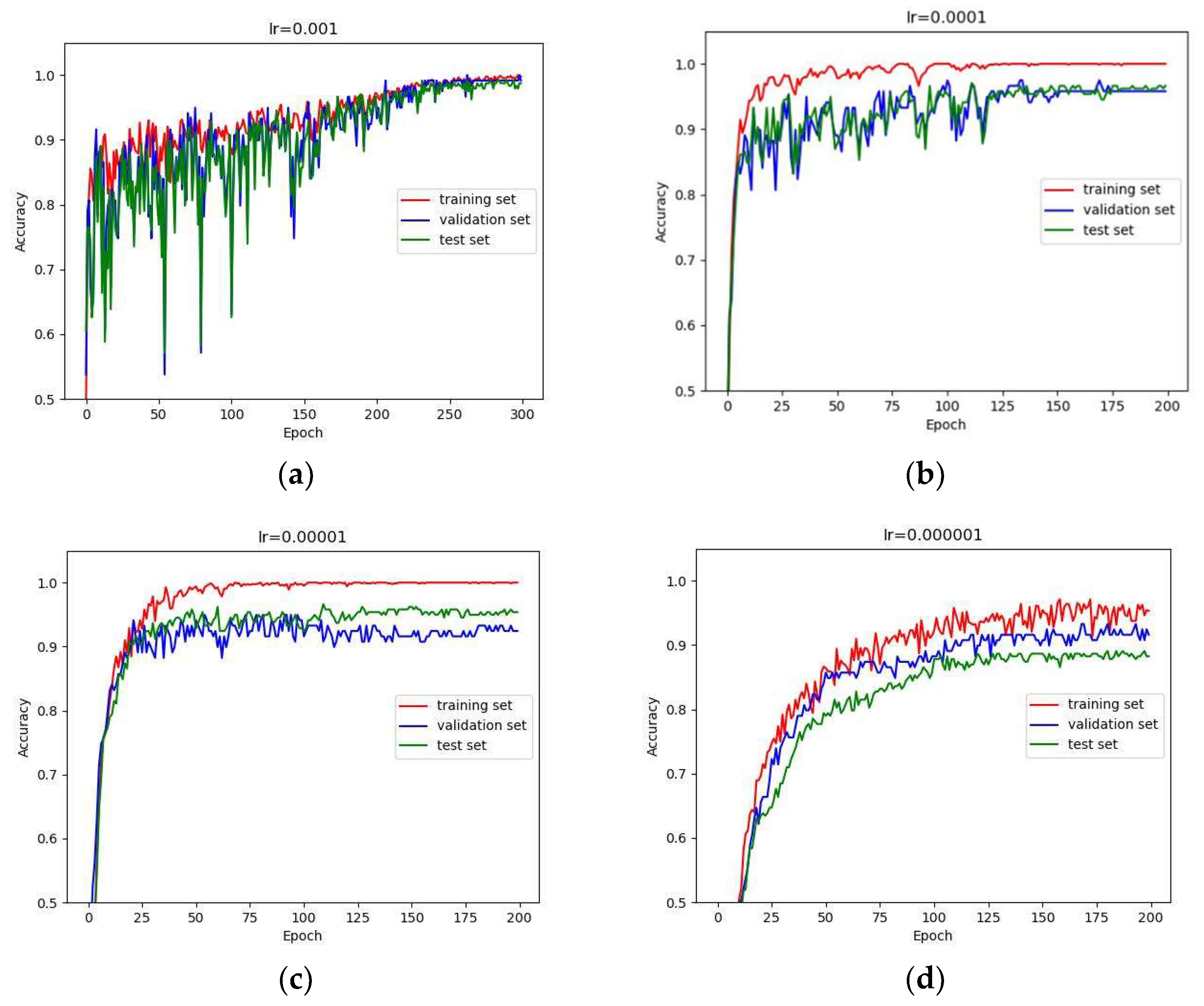
We used a different initial learning rate to train the network, and the results are shown in
Figure 5.
Table 5 shows the accuracy and loss of this dataset on different networks.
In
Table 5, Lr is the learning rate when the network converges; acc is the accuracy rate; train_loss, valid_ loss represent the loss on the training set and validation set, respectively; train_acc, valid_acc, test_acc represent the accuracy on the training set, validation set and test set, respectively. The calculation rule for accuracy is shown in (8):
: true positive, indicating the prediction of positive cases as positive cases; : false positive, indicating the prediction of negative cases as positive cases; : true negative, indicating the prediction of negative cases as negative cases; : false negative, indicating the prediction of positive cases as negative cases.
When the network reaches its optimum, its accuracy on the test set is 98.3%, and our detailed data for this result are organized in
Table 6.
In
Table 6, “A, B, C, D” represent different categories, whose corresponding nitrite concentrations are 0.05, 0.10, 0.15, and 0.20 mg/L, in order; “actual” is the actual concentration category; and “predict” represents the result predicted by the network.
According to
Table 6, we calculated the number of TP, FN, FP, and TN in different categories and accuracy, sensitivity, and specificity on different categories, as shown in
Table 7.
In
Table 7, acc, sens, and spec represent accuracy, sensitivity, and specificity, respectively. The calculation rules for sensitivity and specificity are shown in (9) and (10):
The image used in the above experiment had obvious reflections and shadows, and it was speculated that these features may affect the classification performance of the network; therefore, the preprocessing method of the dataset was adjusted, the areas in the test tube that do not contain reflective parts were captured, and the subsequent alternative processing methods remained unchanged; the example is shown in
Figure 6, and the results are shown in
Table 8.
In addition, we compared the application of chemical colorimetry in actual aquaculture. We found 10 observers (of which observer 1 and observer 2 were fishery workers) to discriminate the selected 30 water samples by chemical colorimetry. These water samples consisted of water samples from the real environment and simulated water samples, and their concentrations were examined with a spectrophotometer. In order to avoid as much as possible the negative influence of the dim environment on the judgment process, we chose the experimental environment on a sunny day with plenty of light. The experimental results are shown in
Table 9.
4. Discussion
Figure 5 shows the convergence of the network with different initial learning rates. When the initial learning rate was 0.001, the accuracy curve of the network fluctuated greatly in the first half of the training period, and converged near the 250th epoch (as shown in (a)). When the initial learning rate was 0.0001, 0.00001, and 0.000001, the accuracy curve of the network converged near the 125th epoch (as shown in (b), (c), and (d)). Even if learning rate warming up is used, it is still necessary to adjust the initial learning rate in order to accelerate network convergence and achieve better results.
After replacing some residual blocks with the ResNeXt module, the performance of the network improved, and the accuracy on the training set, validation set, and test set increased by 0.8%, 0.6%, and 0.5%, respectively. When using image datasets with reflections and shadows for training, adding the SE attention mechanism to the network resulted in a 1% increase in classification accuracy. On the contrary, adding the CBAM attention mechanism resulted in a 0.8% decrease in classification accuracy.
After changing the preprocessing method of the dataset and extracting parts of the image that do not contain reflections or shadows for training, the results indicate that the network’s performance is worse than before.
The experimental results indicate that the features of the dataset in this experiment are concentrated on channel features; therefore, when adding SE, the weight assignment of feature channels in the network is very close to the situation without SE. However, after adding CBAM, the network’s attention to the spatial features of the image reduces the weight of channel features in the image, leading to a certain degree of decrease in the classification accuracy of the network and an increase in losses. The process of cropping the parts of the dataset image that do not contain reflections or shadows, although removing irrelevant features in the image, makes the network only focus on local features in the original data and cannot learn global features well, resulting in a decrease in classification performance.
We introduced two existing detection methods in the Introduction section: chemical colorimetry and spectrophotometry. The chemical colorimetric method depends not only on ambient light but also on the sensitivity of the human eye to color, so the results of judgments vary between people and environments. In the field of aquaculture, this method also depends on work experience. As far as the comparison experiment set up in this experiment is concerned, the accuracy of the judgment results (basically around 50%) of the people with no working experience in the fishery is significantly lower than that of the fishery workers. And the highest accuracy of the judgment results of fishery workers is only 80%. The accuracy of chemical colorimetry is lower than that of our method. Under standard operating conditions, the spectrophotometer used in the spectrophotometric method can achieve a measurement accuracy of more than 99%, or even 100%, which is highly reliable. We agree that the spectrophotometric method is superior to our method in terms of measurement accuracy.
The materials used in the practical application of this method include nitrite detection reagents, cameras, and computers. The price of nitrite detection reagents is CNY 13.5, which can be used 50–60 times, and the price of cameras is CNY 89. Moreover, as a common household device, we can exclude computers from the cost of this method. In this way, compared to the chemical colorimetric method, the cost of our proposed method incurs only the additional cost of the camera, and the detection results are more reliable than the chemical colorimetric method, and compared with spectrophotometers, under standard operating conditions, the accuracy is reduced by 0.7% to 1.7%, but the cost is much lower (the price of a spectrophotometer is generally over CNY 10,000).
In fact, in this study, the original sample dataset we collected already included 38 image sample data from actual aquaculture water bodies. The experimental results also showed that the recognition accuracy of the proposed method can reach 98.3% in real complex environments. Therefore, although the sample dataset of this study mainly consists of simulated water samples, it already includes actual scene water samples and verifies the effectiveness of the method.
5. Conclusions
In this paper, we propose a low-cost and high-precision method for detecting nitrite content in mariculture water environment by combining chemical colorimetry and deep learning. The innovation lies in using the ResNeXt network instead of human eyes to judge the colorimetric results. The experimental results demonstrate that after taking photos of titrated water samples under different lighting conditions and preprocessing the images, the ResNeXt18 + SE attention mechanism network can achieve 98.3% recognition accuracy on the test set. When aquaculture farmers use this method, if they use a camera of the same model as the experiment, there is no need to collect a new dataset. Instead, they only need to capture the titrated water sample and use the trained network to identify the nitrite concentration in the water sample. This method is low-cost and high-accuracy; it can be applied to practical mariculture environments to avoid misjudgments caused by subjective factors and improve mariculture efficiency.
However, there are still some deficiencies, such as the relatively complex steps. In future work, we will focus on expanding the sample size and concentration range, designing end-to-end detection systems and applying this method to other water quality parameter detection methods. In summary, this paper provides a low-cost and high-accuracy technical solution for the online monitoring of aquaculture water quality, which is conducive to promoting the intelligent monitoring of aquaculture water quality.
Author Contributions
Conceptualization, Z.P., Y.B. and W.C.; methodology, Z.P., Y.B. and W.C.; validation, Y.B., W.C. and S.F.; formal analysis, Z.P., Z.C. and J.M.; investigation, Z.C., J.M., Y.B., W.C. and S.F.; resources, Y.B., W.C. and S.F.; writing—original draft preparation, Z.P.; writing—review and editing, Z.P., Z.C., J.M. and Y.B.; funding acquisition, Y.B. and W.C. All authors have read and agreed to the published version of the manuscript.
Funding
This research was funded by the National Natural Science Foundation of China [Grant 32073028], the Open Project of National Key Laboratory [Grant ICT20007], and the Natural Science Foundation of Zhejiang Province [Grant LQ20E030002].
Data Availability Statement
The data presented in this study are available on request from the corresponding author.
Conflicts of Interest
The authors declare no conflict of interest.
References
- Wu, H.; Hou, J.; Wang, X. A review of microplastic pollution in aquaculture: Sources, effects, removal strategies and prospects. Ecotoxicol. Environ. Saf. 2023, 252, 114567. [Google Scholar] [CrossRef] [PubMed]
- Yu, D.; Liu, J.; Zhang, C. Aquaculture Traceability Management with Reference to Fisheries Sustainability. Fish. Sci. 2012, 31, 624–629. [Google Scholar]
- Liu, J.; Liu, H.; Fan, Y.; Tang, X.; Wang, X.; Wang, Y.; Gai, C.; Ye, H. Effects of acute nitrite stress on oxidative stress, energy metabolism and osmotic regulation of Penaeus monodon. J. Fish. China 2023, 47, 42–52. [Google Scholar]
- Wang, S.; Wang, X.; Liu, X.; Jiang, Y.; Cai, Z. Preliminary Study on Ecological Suitability Evaluation Benchmark of Ammonia and Nitrite in Grass Carp Aquaculture Pond. J. Fudan Univ. 2023, 62, 535–541+552. [Google Scholar]
- Wu, D.; Zhou, S.; Liu, Y. Study on rapid detection method of ammonia nitrogen in aquatic environment. Chin. J. Anal. Lab. 2015, 34, 429–432. [Google Scholar]
- Bingio, Y. Learning deep architectures for AI. Found. Trends Mach. Learn. 2009, 2, 1–127. [Google Scholar] [CrossRef]
- Cao, H. Research on Rapid Determination of Organic Matter Concentration in Aquaculture Water Using Multi-Source Spectral Data Fusion. Ph.D. Thesis, Zhejiang University, Hangzhou, China, 2015. [Google Scholar]
- Zhao, C. Development of Multi-Parameter Circuit Monitoring System of Aquaculture Water Quality. Master’s Thesis, Jiangsu University, Zhenjiang, China, 2020. [Google Scholar]
- Song, Y. Study on a Multiplex Spectral In-Situ Water Quality Monitoring Technology. Master’s Thesis, Tianjin University, Tianjin, China, 2022. [Google Scholar] [CrossRef]
- Wang, P.; Liu, B.; Zhang, D.; Du, C.; Li, Z.; Zhang, J.; Zhao, M.; Ma, H.; Wang, W.; Wang, X. Real-time monitoring and early warning of cyanobacteria bloom in source water. Environ. Sci. Technol. 2016, 50, 7950–7958. [Google Scholar]
- Ribeiro, A.R.; Abengozar, M.; Serrano, M.; Reis, C.; Resano, M.; Zaera, E. Development and optimization of a portable microfluidic sensor for nitrite quantification in water. Sens. Actuators B Chem. 2017, 239, 1286–1292. [Google Scholar]
- Ouyang, Q.; Chen, J.; Zhu, L.; Chen, H.; Jiang, X.; Yu, H. Water quality monitoring system based on internet of things and paper microfluidic chip. Comput. Electr. Eng. 2019, 76, 328–337. [Google Scholar]
- Xiong, X.; Zhou, Y.; Mahmood, A.; Hu, X.; Lian, H.; Li, S. Aptamer-functionalized microfluidic chip for high-throughput, quantitative detection of mercury(II) ion in water. Sens. Actuators B Chem. 2019, 288, 497–504. [Google Scholar]
- Fu, G.; Sanjay, S.T.; Dou, M.; Zhou, J.; Xu, F.; Kotaki, M.; Ramakrishna, S.; Ding, B. Low-cost paper-based silver nanoparticle flexible electronics for quality monitoring of drinking water. Npj Flex. Electron. 2019, 3, 1–9. [Google Scholar]
- Krizhevsky, A.; Sutskever, I.; Hinton, G.E. ImageNet classification with deep convolutional neural networks. Assoc. Comput. Mach. 2017, 60, 84–90. [Google Scholar] [CrossRef]
- Zeiler, M.D.; Fergus, R. Visualizing and Understanding Convolutional Networks. In Proceedings of the Computer Vision–ECCV 2014: 13th European Conference, Zurich, Switzerland, 6–12 September 2014. [Google Scholar]
- Simonyan, K.; Zisserman, A. Very Deep Convolutional Networks for Large-Scale Image Recognition. arXiv 2014, arXiv:1409.1556. [Google Scholar]
- Szegedy, C.; Liu, W.; Jia, Y.; Sermanet, P.; Reed, S.; Anguelov, D.; Erhan, D.; Vanhoucke, V.; Rabinovich, A. Going Deeper with Convolutions. In Proceedings of the IEEE Conference on Computer Vision and Pattern Recognition, Columbus, OH, USA, 23–28 June 2014. [Google Scholar]
- Ioffe, S.; Szegedy, C. Batch Normalization: Accelerating Deep Network Training by Reducing Internal Covariate Shift. arXiv 2015, arXiv:1502.03167. [Google Scholar]
- Szegedy, C.; Ioffe, S.; Vanhoucke, V.; Alemi, A. Inception-v4, Inception-ResNet and the Impact of Residual Connections on Learning. In Proceedings of the AAAI Conference on Artificial Intelligence, San Francisco, CA, USA, 4–9 February 2017. [Google Scholar]
- He, K.; Zhang, X.; Ren, S.; Sun, J. Deep Residual Learning for Image Recognition. arXiv 2015, arXiv:1512.03385. [Google Scholar]
- Mnih, V.; Heess, N.; Graves, A. Recurrent Models of Visual Attention. Adv. Neural Inf. Process. Syst. 2014, 27, 3. [Google Scholar]
- Bahdanau, D.; Cho, K.; Bengio, Y. Neural Machine Translation by Jointly Learning to Align and Translate. arXiv 2014, arXiv:1409.0473. [Google Scholar]
- Song, C.; Li, Z.; Li, Y.; Zhang, H.; Jiang, M.; Hu, K.; Wang, R. Research on Blast Furnace Tuyere Image Anomaly Detection, Based on the Local Channel Attention Residual Mechanism. Appl. Sci. 2023, 13, 802. [Google Scholar] [CrossRef]
- Woo, S.; Park, J.; Lee, J.Y.; Kweon, I.S. CBAM: Convolutional Block Attention Module. In Proceedings of the European Conference on Computer Vision (ECCV), Munich, Germany, 8–14 September 2018. [Google Scholar]
- Goyal, P.; Dollár, P.; Girshick, R.; Noordhuis, P.; Wesolowski, L.; Kyrola, A.; Tulloch, A.; Jia, Y.; He, K. Accurate, Large Minibatch SGD: Training ImageNet in 1 Hour. arXiv 2017, arXiv:1706.02677. [Google Scholar]
- Dickson, M.C.; Bosman, A.S.; Malan, K.M. Hybridised Loss Functions for Improved Neural Network Generalisation. In Lecture Notes of the Institute for Computer Sciences, Social Informatics and Telecommunications Engineering; Springer: Cham, Switzerland, 2022. [Google Scholar]
- Szegedy, C.; Vanhoucke, V.; Ioffe, S.; Shlens, J.; Wojna, Z. Rethinking the Inception Architecture for Computer Vision. In Proceedings of the IEEE Conference on Computer Vision and Pattern Recognition (CVPR), Las Vegas, NV, USA, 27–30 June 2016; pp. 2818–2826. [Google Scholar]
Figure 1.
Nitrite content range corresponding to the colorimetric card (the unit is mg/L).
Figure 1.
Nitrite content range corresponding to the colorimetric card (the unit is mg/L).
Figure 2.
The basic network architecture of ResNet18.
Figure 2.
The basic network architecture of ResNet18.
Figure 3.
Residual block.
Figure 3.
Residual block.
Figure 4.
The processing process of sample data. (a) Original image; (b) cropped image; (c) scaled image.
Figure 4.
The processing process of sample data. (a) Original image; (b) cropped image; (c) scaled image.
Figure 5.
The accuracy curves of different learning rates. (a–d) are the initial learning rates of 0.001, 0.0001, 0.00001, and 0.000001, respectively.
Figure 5.
The accuracy curves of different learning rates. (a–d) are the initial learning rates of 0.001, 0.0001, 0.00001, and 0.000001, respectively.
Figure 6.
The processing process of sample data after changing preprocessing method. (a) Original image; (b) cropped image; (c) scaled image.
Figure 6.
The processing process of sample data after changing preprocessing method. (a) Original image; (b) cropped image; (c) scaled image.
Table 1.
Different water quality monitoring methods in aquaculture.
Table 1.
Different water quality monitoring methods in aquaculture.
| Methods | Water Quality Parameters | Authors |
|---|
| spectral techniques | chemical oxygen demand (COD) | Cao [7] |
| multiparameter water quality monitoring robot systems | nitrite | Zhao [8] |
| online monitoring and anomaly detection models | turbidity | Song [9] |
| multiparameter water quality online monitoring and warning systems | water temperature, pH, dissolved oxygen, conductivity, chlorophyll | Wang [10] |
| portable microfluidic sensor | nitrite | Ribeiro [11] |
| Internet of Things-based water quality monitoring systems | mercury | Ouyang [12] |
| DNA aptamer-functionalized microfluidic chips | mercury | Xiong [13] |
| paper-based silver nanoparticle flexible electronics | conductivity, total dissolved solids, chloride | Fu [14] |
Table 2.
Detailed information on the materials used.
Table 2.
Detailed information on the materials used.
| Material | Information |
|---|
| sodium nitrite | standard enforcement: GB/T 633-1994
content: ≥99.0% |
| nitrite test reagent | manufacturer: SOUTH RANCH
number of uses: approximately 50–60 times |
| camera | product model: S-YUE HD1313 |
Table 3.
The detailed parameters of the camera.
Table 3.
The detailed parameters of the camera.
| Parameters | Value |
|---|
| Brightness | 0 |
| Contrast | 32 |
| Hue | 0 |
| Saturation | 64 |
| Clarity | 2 |
| Gamma | 100 |
| White balance | 4600 |
| Backlight contrast | 1 |
| Gain | 0 |
| Power line frequency | 50 Hz |
Table 4.
Comparison of nitrite content detection methods.
Table 4.
Comparison of nitrite content detection methods.
| Methods | Advantages | Disadvantages |
|---|
| spectrophotometry | high accuracy | relatively expensive |
| chemical colorimetry | low cost | relying on rich life experience and susceptible to interference |
| ours | high accuracy and low cost | relatively low accuracy |
Table 5.
Classification results of different network models, and the bolded content indicates that the network works best.
Table 5.
Classification results of different network models, and the bolded content indicates that the network works best.
| Model | Lr | Train_loss | Train_acc | Valid_loss | Valid_acc | Test_acc |
|---|
| ResNet18 | 0.000127 | 0.035768 | 0.982076 | 0.035768 | 0.985679 | 0.973696 |
| ResNeXt18 | 0.000020 | 0.027375 | 0.990373 | 0.032212 | 0.991597 | 0.978992 |
| ResNeXt18 + SE | 0.000176 | 0.026824 | 0.995187 | 0.025154 | 0.991597 | 0.983193 |
| ResNeXt18 + CBAM | 0.000148 | 0.075276 | 0.969916 | 0.051993 | 0.991597 | 0.970588 |
| Inception-v3 | 0.001227 | 0.011440 | 0.997593 | 0.101131 | 0.957983 | 0.941176 |
| Vgg16 | 0.000012 | 0.001108 | 1.0 | 0.108087 | 0.966387 | 0.962185 |
Table 6.
The confusion matrix for the prediction results of ResNeXt18+SE.
Table 6.
The confusion matrix for the prediction results of ResNeXt18+SE.
| Confusion Matrix | Predict |
|---|
| A | B | C | D |
|---|
| Actual | A | 92 | 4 | 0 | 0 |
| B | 0 | 49 | 6 | 0 |
| C | 0 | 0 | 49 | 2 |
| D | 0 | 0 | 0 | 36 |
Table 7.
The number of TP, FN, FP, TN in different categories, and accuracy, sensitivity, and specificity in different categories.
Table 7.
The number of TP, FN, FP, TN in different categories, and accuracy, sensitivity, and specificity in different categories.
| | TP | FN | FP | TN | Acc | Sens | Spec |
|---|
| A | 92 | 4 | 0 | 234 | 0.983193 | 0.958333 | 1.0 |
| B | 49 | 6 | 4 | 234 | 0.983193 | 0.890909 | 0.983193 |
| C | 49 | 2 | 6 | 232 | 0.974790 | 0.960784 | 0.974790 |
| D | 36 | 0 | 2 | 236 | 0.991597 | 1.0 | 0.991597 |
Table 8.
Classification results of different network models after adjusting the dataset, and the bolded content indicates that the network works best.
Table 8.
Classification results of different network models after adjusting the dataset, and the bolded content indicates that the network works best.
| Model | Lr | Train_loss | Train_acc | Valid_loss | Valid_acc | Test_acc |
|---|
| ResNeXt18 | 0.000203 | 0.031355 | 0.990373 | 0.113633 | 0.983193 | 0.941176 |
| ResNeXt18 + SE | 0.000079 | 0.056776 | 0.980746 | 0.070939 | 0.974790 | 0.957983 |
| ResNeXt18 + CBAM | 0.000122 | 0.133269 | 0.954272 | 0.128041 | 0.949580 | 0.941176 |
Table 9.
Identification results of 30 water samples by different observers using the chemical colorimetric method (* indicates that the observer is a fishery worker, bolding of the Observer 1 line indicates the best results, and bolding of the Observer 7 line indicates the worst results).
Table 9.
Identification results of 30 water samples by different observers using the chemical colorimetric method (* indicates that the observer is a fishery worker, bolding of the Observer 1 line indicates the best results, and bolding of the Observer 7 line indicates the worst results).
| | Number of Correct Judgments | Accuracy |
|---|
| Observer 1 * | 24 | 80.0% |
| Observer 2 * | 23 | 76.7% |
| Observer 3 | 14 | 46.7% |
| Observer 4 | 15 | 50.0% |
| Observer 5 | 14 | 46.7% |
| Observer 6 | 13 | 43.3% |
| Observer 7 | 11 | 36.7% |
| Observer 8 | 17 | 56.7% |
| Observer 9 | 14 | 46.7% |
| Observer 10 | 16 | 53.3% |
| Disclaimer/Publisher’s Note: The statements, opinions and data contained in all publications are solely those of the individual author(s) and contributor(s) and not of MDPI and/or the editor(s). MDPI and/or the editor(s) disclaim responsibility for any injury to people or property resulting from any ideas, methods, instructions or products referred to in the content. |
© 2023 by the authors. Licensee MDPI, Basel, Switzerland. This article is an open access article distributed under the terms and conditions of the Creative Commons Attribution (CC BY) license (https://creativecommons.org/licenses/by/4.0/).

 ,
, 


