Article

Research on the Construction of an Efficient and Lightweight Online Detection Method for Tiny Surface Defects through Model Compression and Knowledge Distillation

1
Key Laboratory of Advanced Manufacturing Technology, Ministry of Education, Guizhou University, Guiyang 550025, China
2
School of Mechanical Engineering, Guizhou University, Guiyang 550025, China
3
School of Mechanical Engineering, Guiyang University, Guiyang 550005, China
4
Department of Mechanical and Manufacturing Engineering, Faculty of Engineering, Universiti Putra Malaysia (UPM), Serdang 43400, Malaysia
5
Department of Mechanical and Electronic Engineering, Guizhou Communications Polytechnic, Guiyang 551400, China
*
Authors to whom correspondence should be addressed.
Electronics 2024, 13(2), 253; https://doi.org/10.3390/electronics13020253
Submission received: 22 November 2023 / Revised: 21 December 2023 / Accepted: 3 January 2024 / Published: 5 January 2024
(This article belongs to the Special Issue Deep Learning in Computer Vision and Image Processing)

Abstract

:
In response to the current issues of poor real-time performance, high computational costs, and excessive memory usage of object detection algorithms based on deep convolutional neural networks in embedded devices, a method for improving deep convolutional neural networks based on model compression and knowledge distillation is proposed. Firstly, data augmentation is employed in the preprocessing stage to increase the diversity of training samples, thereby improving the model’s robustness and generalization capability. The K-means++ clustering algorithm generates candidate bounding boxes, adapting to defects of different sizes and selecting finer features earlier. Secondly, the cross stage partial (CSP) Darknet53 network and spatial pyramid pooling (SPP) module extract features from the input raw images, enhancing the accuracy of defect location detection and recognition in YOLO. Finally, the concept of model compression is integrated, utilizing scaling factors in the batch normalization (BN) layer, and introducing sparse factors to perform sparse training on the network. Channel pruning and layer pruning are applied to the sparse model, and post-processing methods using knowledge distillation are used to effectively reduce the model size and forward inference time while maintaining model accuracy. The improved model size decreases from 244 M to 4.19 M, the detection speed increases from 32.8 f/s to 68 f/s, and mAP reaches 97.41. Experimental results demonstrate that this method is conducive to deploying network models on embedded devices with limited GPU computing and storage resources. It can be applied in distributed service architectures for edge computing, providing new technological references for deploying deep learning models in the industrial sector.

1. Introduction

In the manufacturing process of industrial products, various factors, such as the influence of processing equipment on automated production lines, manufacturing processes, and the surrounding environment, can lead to the occurrence of a wide range of defects in the processed products. Therefore, the effective quality inspection of the product manufacturing process is of significant practical importance for businesses aiming to enhance quality, reduce costs, and increase efficiency [1,2,3]. Machine vision-based technology for detecting surface defects in products has become increasingly mature and is widely used in critical industrial sectors such as the aerospace, electronics, machinery manufacturing, and automotive industries. In general, conventional industrial quality inspection relies on the characteristics and properties of surface defects to design appropriate imaging schemes. Subsequently, defect areas are separated using techniques like region cropping and edge detection. Specific techniques such as histogram of oriented gradient (HOG) and local binary pattern (LBP) are employed for feature extraction, which is then input into a classifier, or threshold methods are used to determine defect types. In [4], the authors utilized the local maximum variance method to effectively segment solar cell images and identify busbars. They proposed a positioning algorithm that combines integral projection with grayscale centroid. They designed a support vector machine (SVM) classifier with a radial basis function (RBF) as the kernel function. Experimental results demonstrated that this method achieved a recognition rate of over 90% for common defects in solar cells. In [5], an image processing technique was used to develop a rust-defect detection method for earthquake hammers. This method combined histogram equalization, morphological processing, and knowledge of the RGB color model. It involved template matching between the normal state of the earthquake hammer and its rusted condition to detect rust defects. Experimental results indicated that this method achieved an accuracy of around 80% in detecting rust on earthquake hammers. In [6], a detection method was proposed to identify defects in industrial products with a center-symmetric distribution pattern. This method is an improved version of the Hough transform-based detection approach. Experimental results demonstrated that this algorithm can effectively address the issue of undetectable defects caused by the similarity between the target and the background. In [7], a fabric defect detection method was proposed based on HOG and support vector machine (SVM). In this method, each block-based feature of the image was encoded using HOG, which is insensitive to variations in lighting and noise. Feature extraction was carried out using the AdaBoost algorithm, and an SVM was used for the classification of fabric defects. Experimental results have demonstrated the effectiveness of this algorithm. However, industrial production environments often exhibit a certain level of complexity and unpredictability. For instance, factors such as a high similarity between defects and the background, significant scale variations, a wide range of defect types, a low image contrast, and high levels of noise can all impact the accuracy of traditional defect detection methods. As a result, traditional methods of quality inspection are no longer able to meet the current demands of production.
The advent of convolutional neural networks (CNNs) has transformed this landscape. Thanks to their robust feature extraction capabilities, factors such as object shape, size, texture, background, and image quality are no longer significant obstacles in quality inspection with the assistance of CNNs. CNNs can replace traditional feature extractors and classifiers from feature learning theories, eliminating the need for the complex preprocessing of raw images and streamlining the detection process. Currently, target detection algorithms with a CNN as the backbone have made significant breakthroughs in various fields. From a practical standpoint, deep learning-based target detection algorithms are highly consistent with traditional surface quality inspection. Structurally, this detection method can be categorized into two-stage networks, represented by the region-based convolutional neural network (R-CNN) series [8], which involves candidate box generation and classification, and one-stage networks, represented by the you only look once (YOLO) series [9,10,11,12,13,14,15,16] and single shot multibox detector (SSD) [17], which directly predict target categories and positions using the features extracted from the backbone network.
Deep learning-based object detection algorithms have gradually started to be applied in various product quality inspection scenarios. In [18], a fabric quality defect detection network tailored for complex background textures was proposed. Gabor kernels were embedded into the faster R-CNN network. A two-stage training approach based on genetic algorithm (GA) and backpropagation was designed to train the new faster GG R-CNN model. The resulting model exhibited a 15.59% improvement in mean average precision (mAP) compared to the original network model. In [19], a method for casting defect recognition based on an improved YOLOv3 model was proposed. It employed guided filtering techniques to enhance the defect images in defect recognition (DR) images, resulting in standardized defect samples. This was achieved by incorporating dual-density convolution layers into YOLOv3, reducing the defect detection rate and enhancing the network accuracy. The improved network model exhibited a 26.1% increase in mAP compared to YOLO v3. It also showed faster convergence and better convergence characteristics. In [20], in response to the challenges of a low detection accuracy, poor interference resistance, and slow detection speed in traditional tunnel lining defect detection methods, a novel deep learning-based network model called YOLOv4-ED was proposed. It incorporated the depthwise separable convolution (DSC) block to reduce the model’s storage space and enhance detection efficiency. Ultimately, the model achieved a mAP of 81.84%. In [21], a surface defect detection method based on the MobileNet-SSD network was proposed. Model simplification was achieved through adjustments to the network structure and parameters. This method was applied to the typical defect detection on the sealing surfaces of containers in a filling production line. Compared to traditional machine learning and lightweight network methods, the proposed approach offers more accurate and faster defect detection on the container surfaces. In [22], a computer vision method based on deep learning is proposed. This method seamlessly integrates Mask-RCNN, U-net, and an innovative crack quantification technique, considering the actual distribution and orientation of dense microcracks. It is used for the identification, quantification, and visualization of microcracks in high-performance fiber-reinforced cementitious composites (HPFRCCs). The presented method has exhibited promising performance in identifying and quantifying dense microcracks in HPFRCCs, fully considering the interconnection and orientation of the microcracks during the quantification process. Generally, one-stage detection networks typically do not achieve the same level of accuracy as two-stage networks. However, they offer the advantage of simpler detection structures and an extremely high detection efficiency compared to two-stage networks. This makes them more scalable and versatile in diverse industrial settings.
In response to the current issues of poor real-time performance, high computational costs, and the excessive memory usage of object detection algorithms based on deep convolutional neural networks in embedded devices, this paper uses a one-stage detection network as a technical starting point to build an online model for the surface quality inspection of products. The goal is to enhance detection accuracy by modifying the network structure and adjusting network parameters, finding a suitable balance between detection accuracy and speed. Moreover, considering the demanding hardware and production conditions in some industrial sectors, this paper incorporates the ideas of model pruning and knowledge distillation into the design of the product quality online inspection model. This is performed to improve the model’s applicability in various scenarios, enabling its deployment on automated production lines. This approach contributes to the construction of a digital twin model for in-process product surface quality inspection in a rule-based manner.

2. Pre-Treatment and Methods

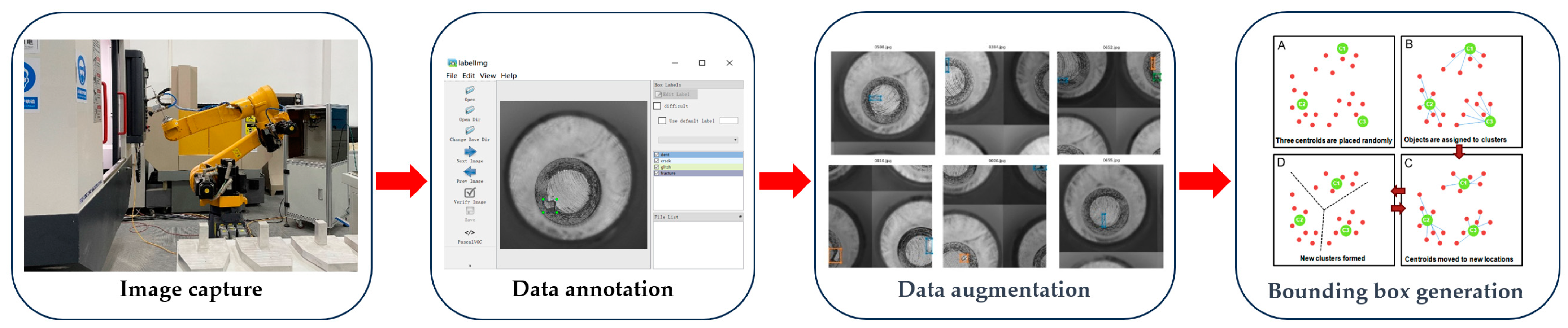
2.1. Sample Pre-Treatment

In industrial production lines, the collected images often exhibit characteristics of stability in shape, singularity, and a limited number of samples. This article focuses on validating the feasibility of the proposed method using an eccentric conical workpiece as the experimental subject. The machining quality at the eccentric convex portion of this workpiece directly determines the precision of subsequent assembly processes, making the online quality control of utmost importance. In the experiments described in this paper, a charge coupled device (CCD) camera was used to capture 1200 images of tiny defects on the surface of aerospace products on an automated production line. These defects included “Dent”, “Crack”, “Glitch”, and “Fracture”. To meet the real-time and accuracy requirements of the industrial domain, the original image dimensions were first normalized to 416 × 416 pixels. This resizing enhances model detection speed without compromising useful image information. Subsequently, the normalized images were divided into training and testing sets, with data augmentation applied to the training set images. Finally, considering the locations and sizes of defects in all defect labels, a clustering approach was used to initialize the sizes of anchor boxes in the detection network, as part of the defect sample preprocessing. The image preprocessing workflow is detailed in Figure 1.

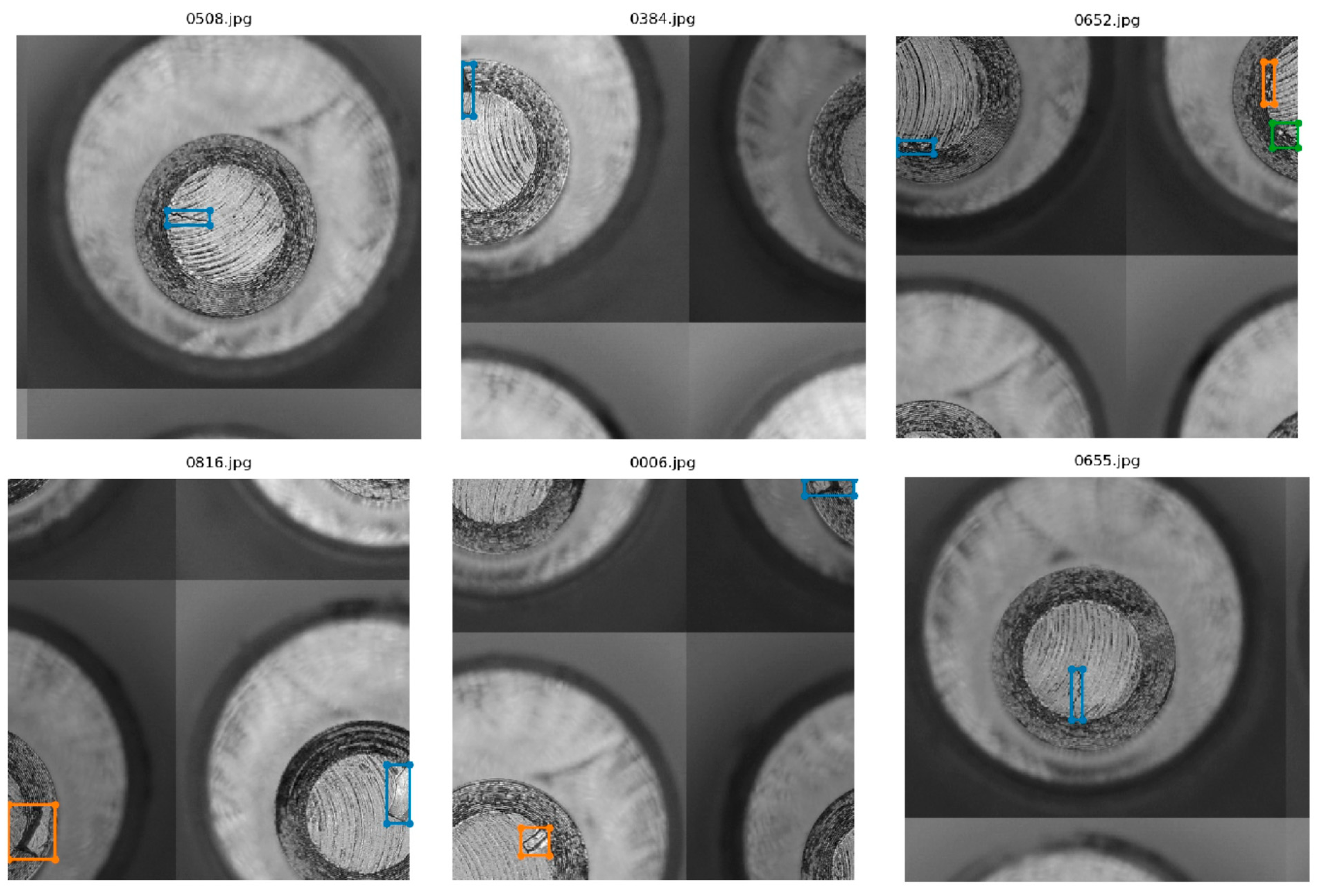
2.1.1. Data Augmentation Methods

When the sample data in an image dataset are too small, the situation can lead to the overfitting of the deep learning neural network model. To prevent this from happening, data augmentation methods can be effectively used to reduce overfitting, make the model better suited for new samples, reduce the model’s reliance on certain attributes, and improve its robustness and generalization ability. In this study, a supervised data augmentation method called mosaic [12] was selected. This method involves reading four sample images at a time and randomly scaling, cropping, and arranging them. The images are combined, and the bounding boxes are combined after being placed in four different positions. This approach enriches the detection dataset, particularly by adding many small objects through random scaling, thereby addressing the issue of target scale imbalance in the original dataset and improving the network’s robustness. The data from the four sample images are directly processed at the BN layer, allowing for a smaller mini-batch size. This enables effective training on a single GPU. Specific examples of data samples using the mosaic data augmentation method are shown in Figure 2.

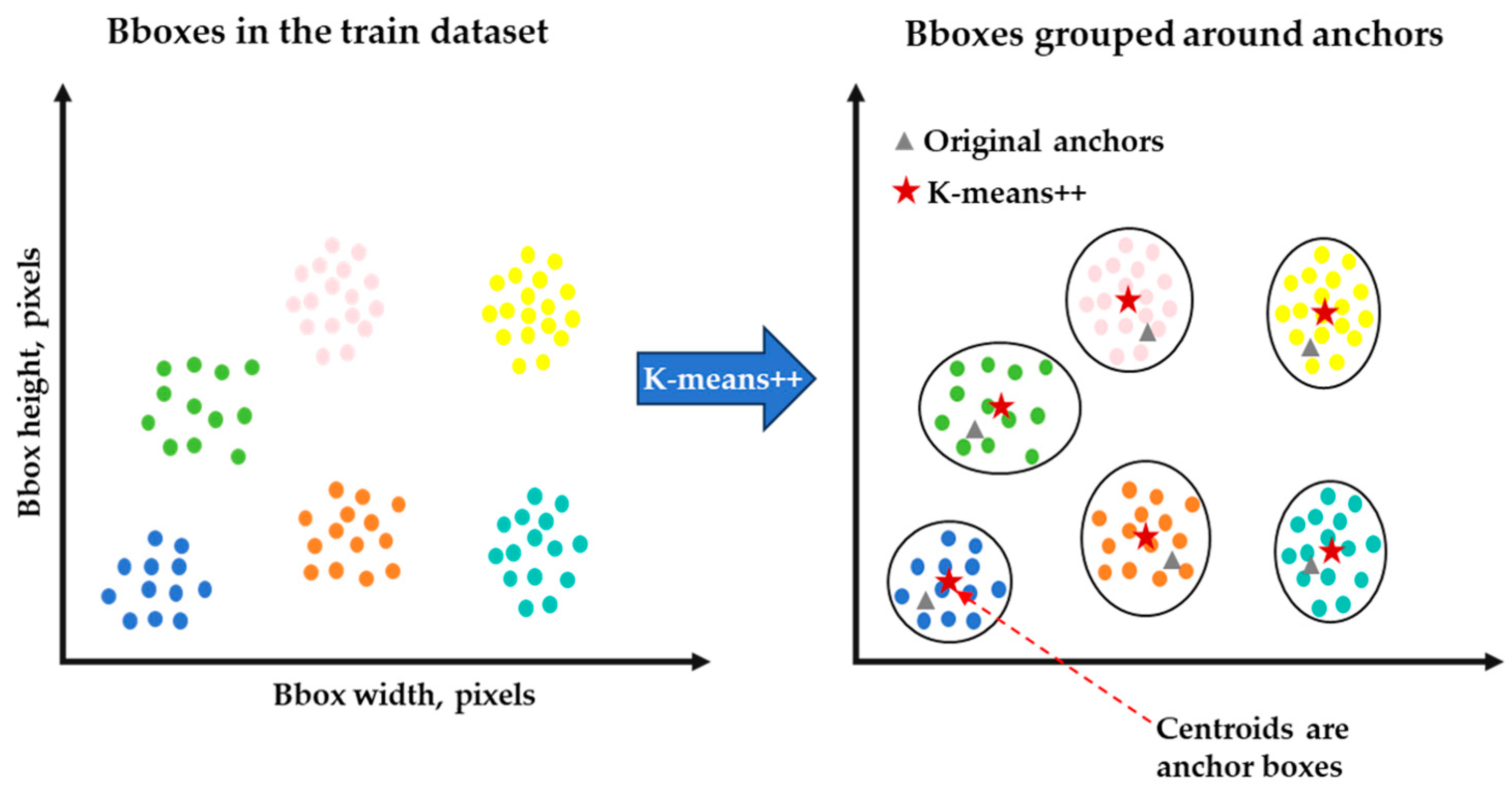
2.1.2. Bounding Box Generation Methods

The process of generating anchor box for object detection networks helps in defect classification prediction, enabling the model to select finer features at an earlier stage. In the YOLO series of object detection networks, the default sizes for anchor boxes are (10, 13), (16, 30), (33, 23), (30, 61), (62, 45), (59, 119), (116, 90), (156, 198), and (373, 326), totaling nine different sizes. However, these sizes may not be tailored to specific datasets. In this study, the K-means++ method was used to perform clustering analysis on the ground-truth boxes in the image labels. The core idea of this method is to select data points that are as far apart as possible from the initial cluster centers, effectively addressing the problem of over-reliance on the cluster center selection method in traditional K-means. Subsequently, anchor boxes that are objective and representative are chosen based on the clustering results. The specific process of determining the initial estimation of anchor boxes using the K-means++ clustering algorithm is illustrated in Figure 3.
The specific implementation steps of this process are as follows:
Step 1: Randomly select the width and height of any ground-truth box in a label as the initial cluster center, c 1 .
Step 2: Calculate the shortest Euclidean distance, represented as D ( x ) , between all ground-truth boxes and the current existing cluster centers. Calculate the probability of each ground-truth box being chosen as the next cluster center using the formula D ( x ) 2 / D ( x ) 2 , and select the next cluster center using a roulette wheel selection.
Step 3: Repeat the process from Step 2 until you have selected K cluster centers z 1 , z 2 ,   , z k .
Step 4: Calculate the distance d i j ( y j , z i ) between each ground-truth box y i and each cluster center, y j y 1 ,   , y n , where n is the number of samples. The distance calculation is represented as:
d i s t a n c e ( b o x , c e n t r o i d ) = 1 I o U ( b o x , c e n t r o i d )
where “ b o x ” represents the set of ground-truth boxes, “ c e n t r o i d ” represents the set of cluster centers, and “ I o U ( b o x , c e n t r o i d ) ” represents the Intersection over Union (IoU) between ground-truth boxes and cluster centers.
Step 5: Based on the principle of minimizing distance, classify the ground-truth boxes. For each ground-truth box y j , if d i j is the minimum distance, then y j is assigned to class e i , meaning y j e i . Subsequently, calculate the mean z i of all samples in class e i , and this mean is used as the new cluster center for class e i , represented as:
z i = 1 N i y j e i y i , i = 1,2 ,   , k
where N i is the number of samples belonging to class e i .
Step 6: If the cluster centers do not change significantly, the clustering process is completed. Otherwise, go back to Step 3 and continue iterating.
The anchor box sizes obtained using the K-means++ method are in the order as follows: (15, 42), (26, 45), (41, 17), (36, 41), (48, 34), (72, 70), (161, 109), (113, 161), and (184, 172). These anchor box sizes will be used for generating the initial anchors in the detection network.

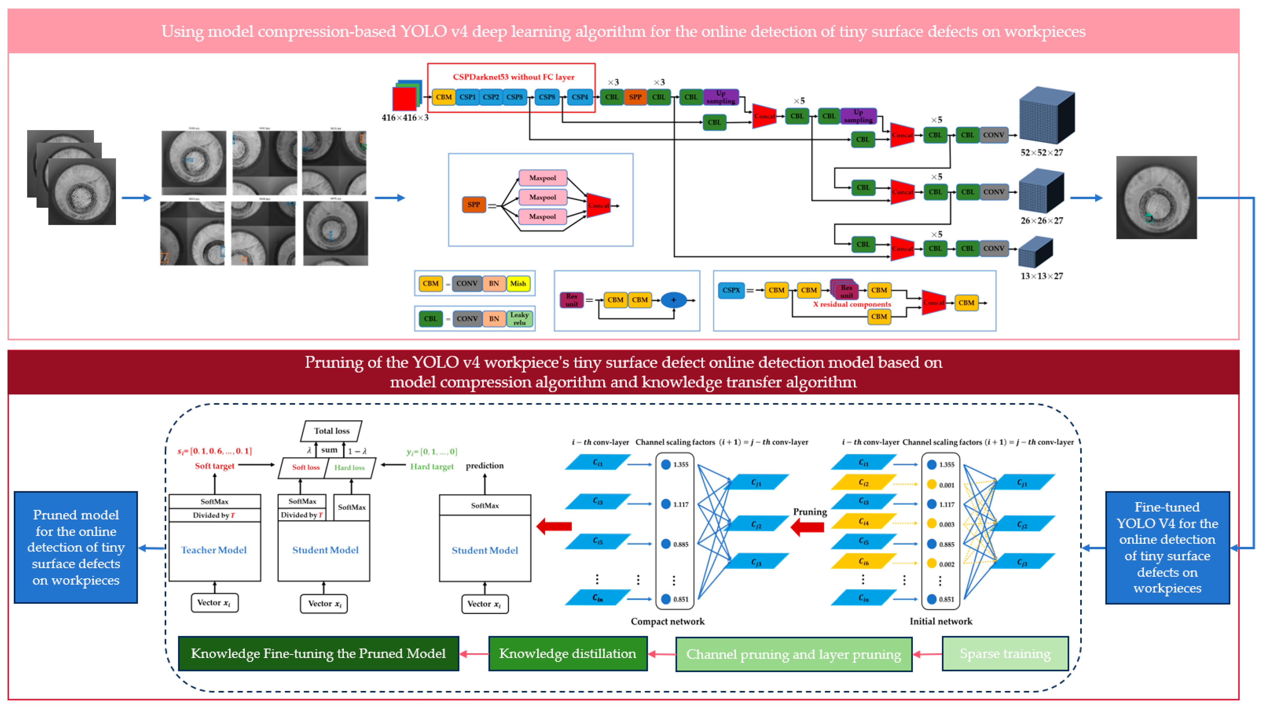
2.2. Using Model Compression-Based YOLOv4 Deep Learning Algorithm for the Online Detection of Tiny Surface Defects on Workpieces

2.2.1. Overall Technical Route

This study aims to achieve the online detection of tiny surface defects on workpieces and mark the defect locations using embedded devices. The technical route of the proposed method is depicted in Figure 4. In this research:
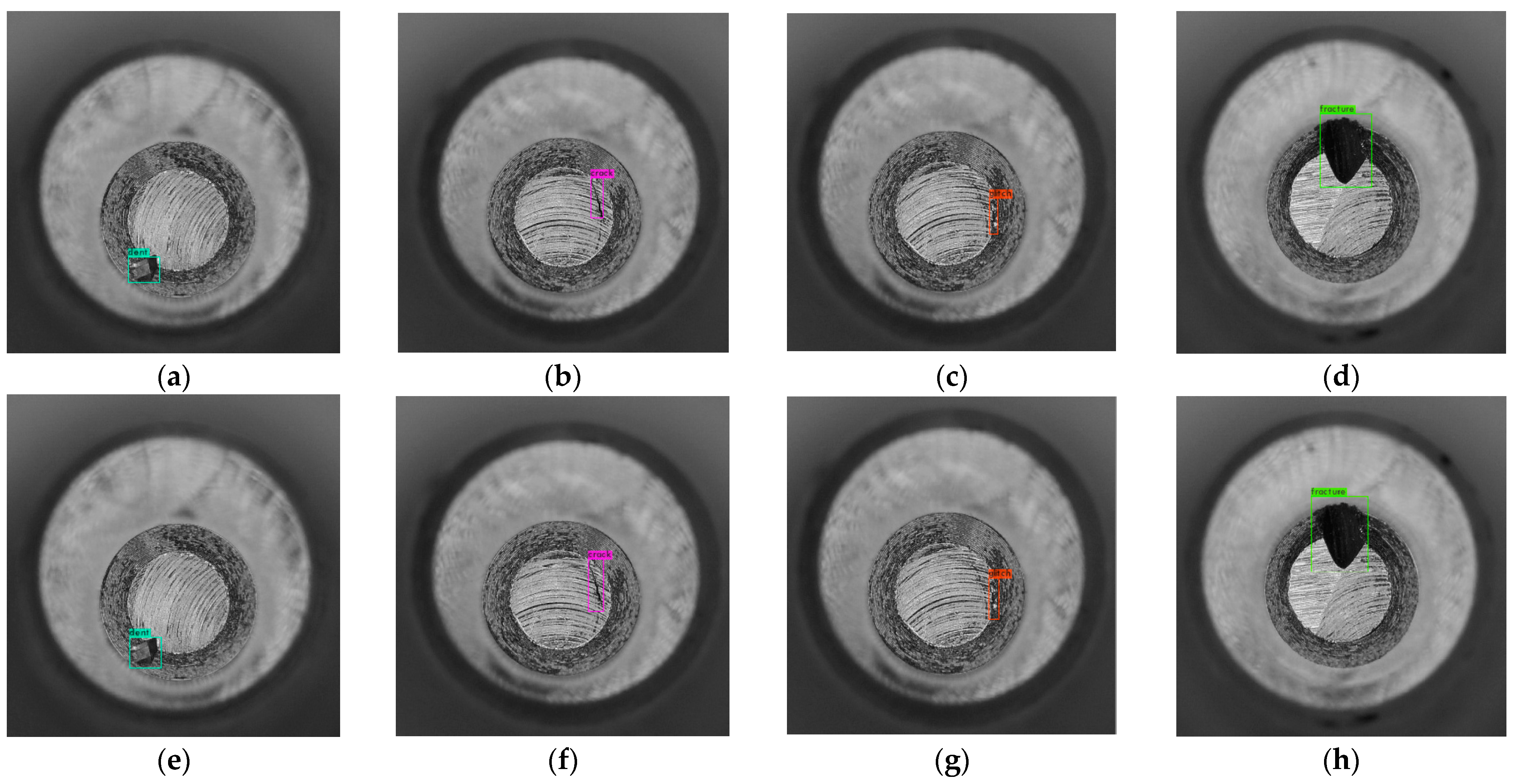
  • Initially, manually labeled surface defect data for workpieces were used to train an improved YOLOv4 object detection network. This training process incorporated transfer learning, enabling the rapid detection and labeling of tiny surface defects on workpieces.
  • After training the YOLOv4 model for workpiece surface defect detection, model compression and knowledge transfer techniques were applied. This involved model pruning and knowledge distillation algorithms, simplifying the model’s structure and parameters while maintaining model accuracy.
The ultimate objective of this research is to simplify and optimize the process of detecting and marking tiny surface defects on workpieces using embedded devices.

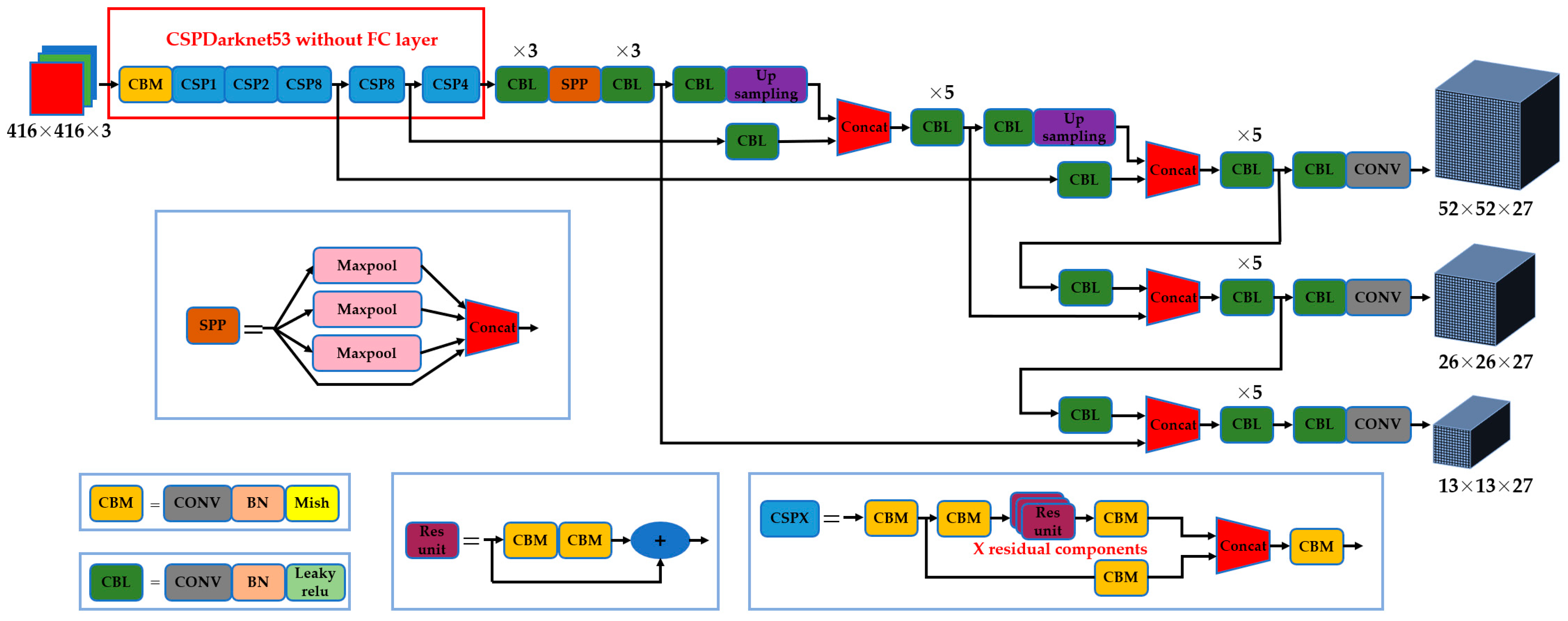
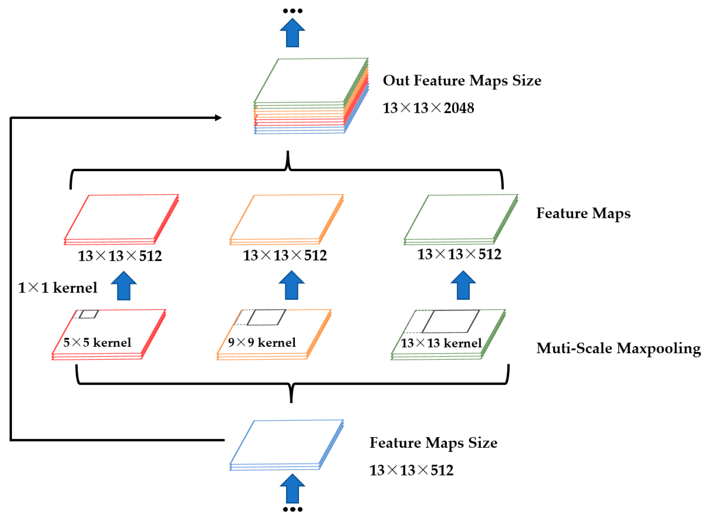
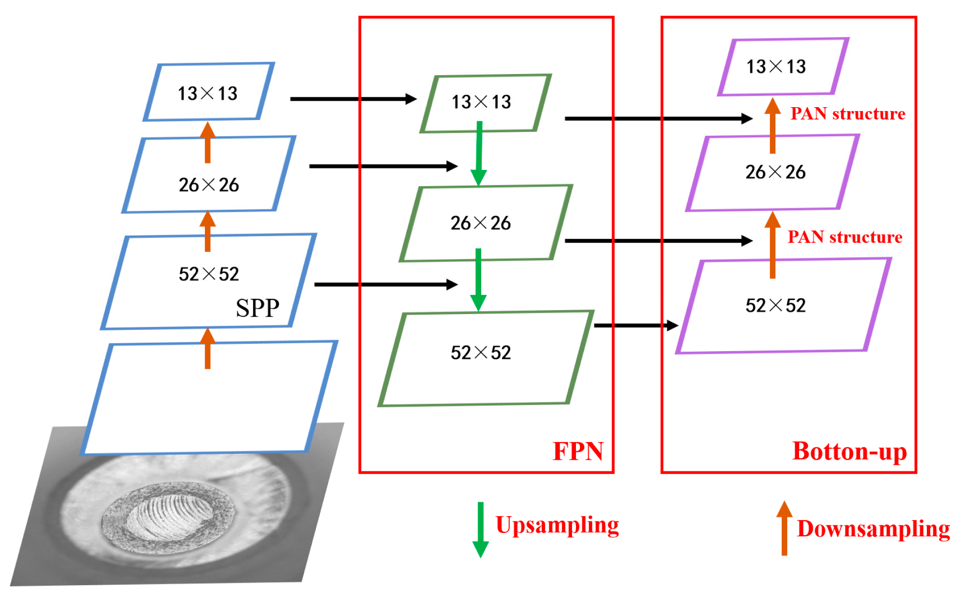
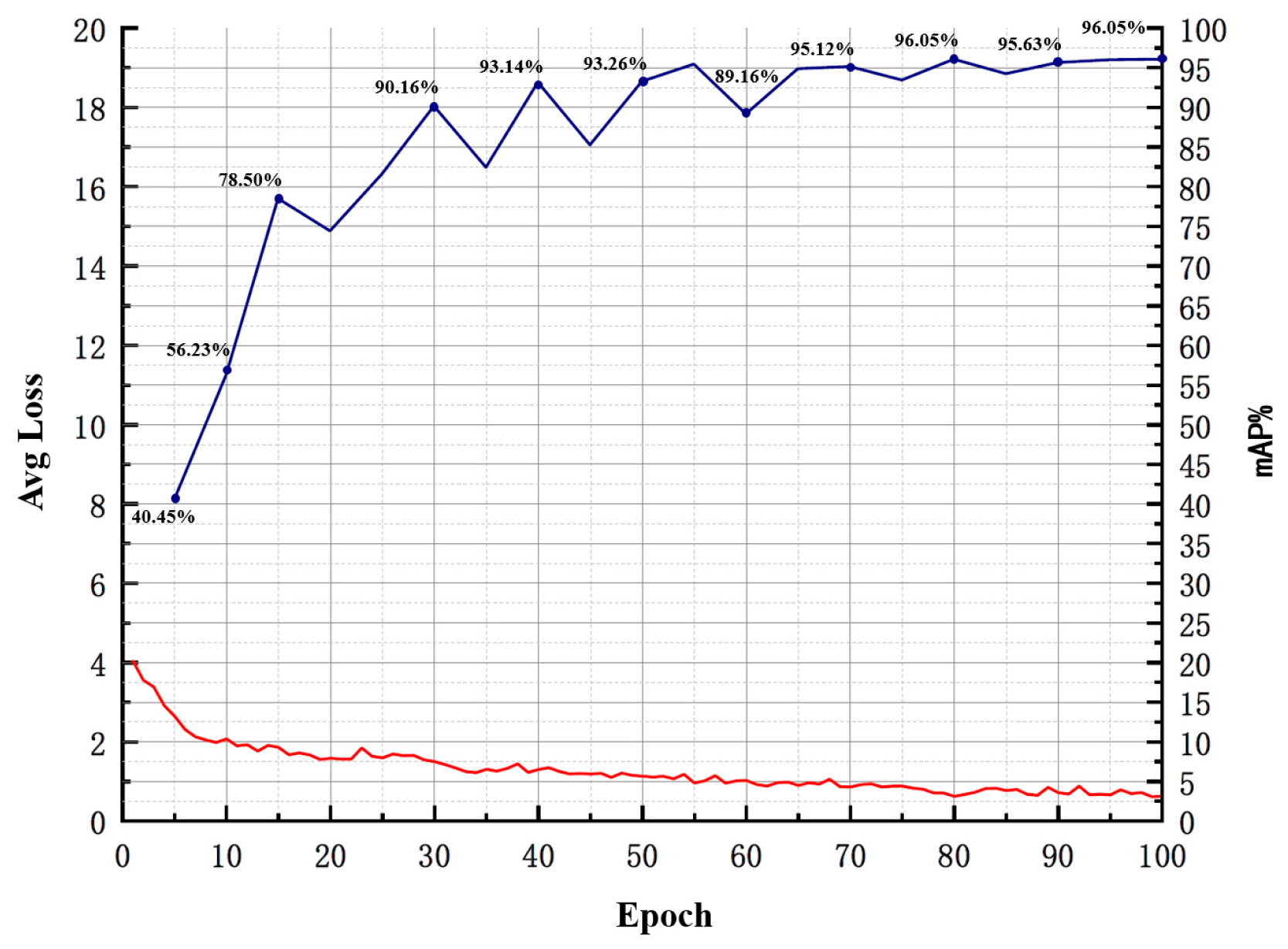
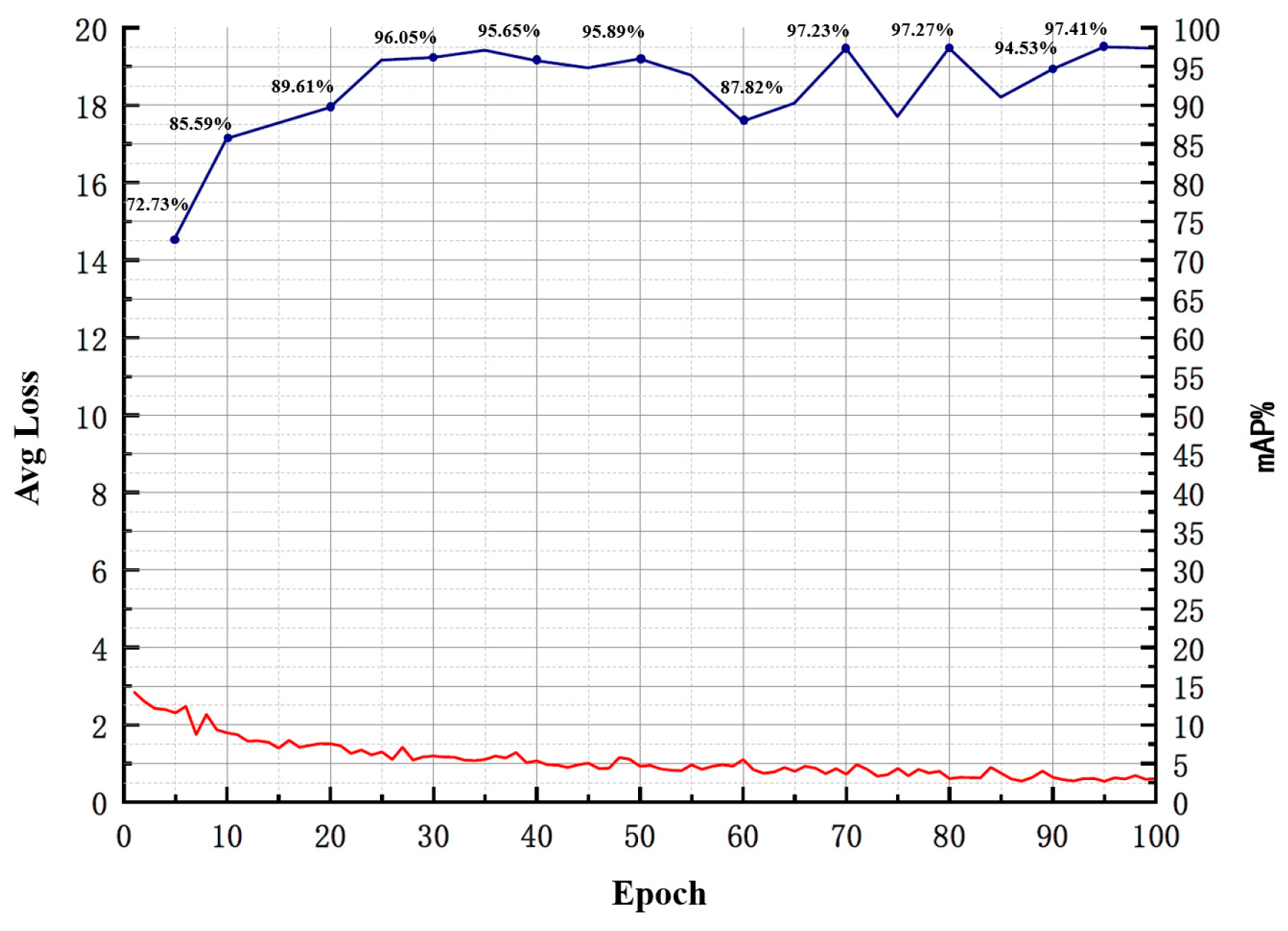
2.2.2. Construction of a Workpiece’s Tiny-Surface-Defect Online Detection Model Based on YOLOv4

The YOLO network is an object detection algorithm based on regression. It offers fast detection speeds and can perform end-to-end object detection and recognition, making it highly effective in fast real-time object detection tasks. In this paper, YOLOv4 is used to identify and label defect categories in images. YOLOv4 was introduced by Alexey Bochkovskiy and his team in 2020. It is an improvement over the YOLOv3 network by combining new algorithmic ideas, enhancing detection efficiency and accuracy, and making it more friendly for detecting small objects.
The YOLOv4 network consists of four main components: the input, Backbone, Neck, and Prediction. Initially, the Backbone main network is used to extract features from the input image. Then, the input image is divided into an S × S grid, and each grid is responsible for detecting targets within it. Each grid predicts B bounding boxes and the probabilities for belonging to C different categories. It also outputs confidence information representing whether the bounding box contains an object and the accuracy of the bounding box. The overall structure of the workpiece surface quality online detection model used in this study is shown in Figure 5.
CSP Darknet53 is a Backbone structure derived from YOLOv3’s main network Darknet53. It adds CSP modules to each major residual block in order to optimize network architecture and address the issue of high-inference computation due to redundant gradient information. CSP Darknet53 includes 5 CSP modules, and each CSP module is preceded by a 3 × 3 convolution kernel with a stride of 2, effectively performing down sampling. Since the Backbone has 5 CSP modules, and the input image is 416 × 416, the pattern of feature map size changes is as follows: 416 → 208 → 104 → 52 → 26 → 13. After passing through 5 CSP modules, a 13 × 13 feature map is obtained. The activation function used in the CSP Darknet53 main network is Mish, while Leaky_ReLU is still used as the activation function in the later parts of the network.
To improve feature fusion in the YOLOv4’s Neck section, a combination of the SPP module and the feature pyramid network with path aggregation network (FPN + PAN) methods is primarily used. Using the SPP module, rather than relying solely on k × k max pooling, effectively increases the reception range of the main features and significantly separates the most crucial contextual features. In this study, within the SPP module, max pooling with different scales K = {1 × 1, 5 × 5, 9 × 9, 13 × 13} was employed, and the resulting feature maps were concatenated. The SPP structure is illustrated in Figure 6.
By employing the FPN with PAN methods, YOLOv4 adds a bottom-up feature pyramid PAN layer behind the FPN layer. The FPN layer conveys strong semantic features from the top down, while the PAN layer conveys strong positional features from the bottom up. By combining these two approaches, the network aggregates parameters from different backbone layers to different detection layers, further enhancing the network’s feature extraction capabilities. The FPN + PAN structure is detailed in Figure 7.
In the prediction part of YOLO v4, the loss function primarily consists of three components: bounding box position loss, confidence loss, and classification loss.
L o s s = L o s s C I o U + L o s s c o n f + L o s s c l s
Part 1: Bounding box position loss, represented as L o s s C I o U , is represented using a regression loss function.
v = 4 π 2 a r c t a n w g t h g t a r c t a n w h
α = v 1 I o U + v
L o s s C I o U = 1 I o U + d 2 c 2 + α v
In the equation, “ v ” represents a parameter that measures aspect ratio consistency; “ w g t ” and “ h g t ” represent the width and height of the ground truth bounding box; ” w ” and “ h ” represent the width and height of the predicted bounding box; “ α ” represents a parameter used for balancing; “ I o U ” represents the intersection over union between the predicted bounding box and the ground truth bounding box; “ c ” represents the diagonal distance of the closure; “ d ” represents the Euclidean distance between the two center points.
Part 2: Confidence loss, represented as L o s s c o n f , is represented using a cross-entropy loss function.
L o s s c o n f = i = 0 S × S j = 0 B I i j o b j C i ^ l o g C i 1 C i ^ l o g 1 C i + λ n o o b j i = 0 S × S j = 0 B I i j n o o b j C i ^ l o g C i 1 C i ^ l o g 1 C i
In the equation, “ S × S ” represents the number of grids into which the input image is divided; “ B ” represents the number of predicted bounding boxes per grid; “ I i j o b j ” represents a value of 1 when the j-th bounding box predicted by the i-th grid detects an object, and 0 otherwise; “ C i ^ ” represents the confidence score of the actual bounding box in the i-th grid; “ C i ” represents the confidence score of the predicted bounding box in the i-th grid; “ λ n o o b j ” represents the weight coefficient for grids that do not contain objects.
Part 3: The classification loss, represented as L o s s c l s , is represented using the cross-entropy loss function.
L o s s c l s = i = 0 S × S I i j o b j C c l a s s e s p i ^ C l o g p i C 1 p i ^ C l o g 1 p i C
In the equation, “ C ” represents the category to which the detected target belongs; “ p i ^ C ” represents the actual probability that the target belongs to category C when detected in the i-th grid; “ p i C ” represents the predicted probability that the target belongs to category C when detected in the i-th grid.

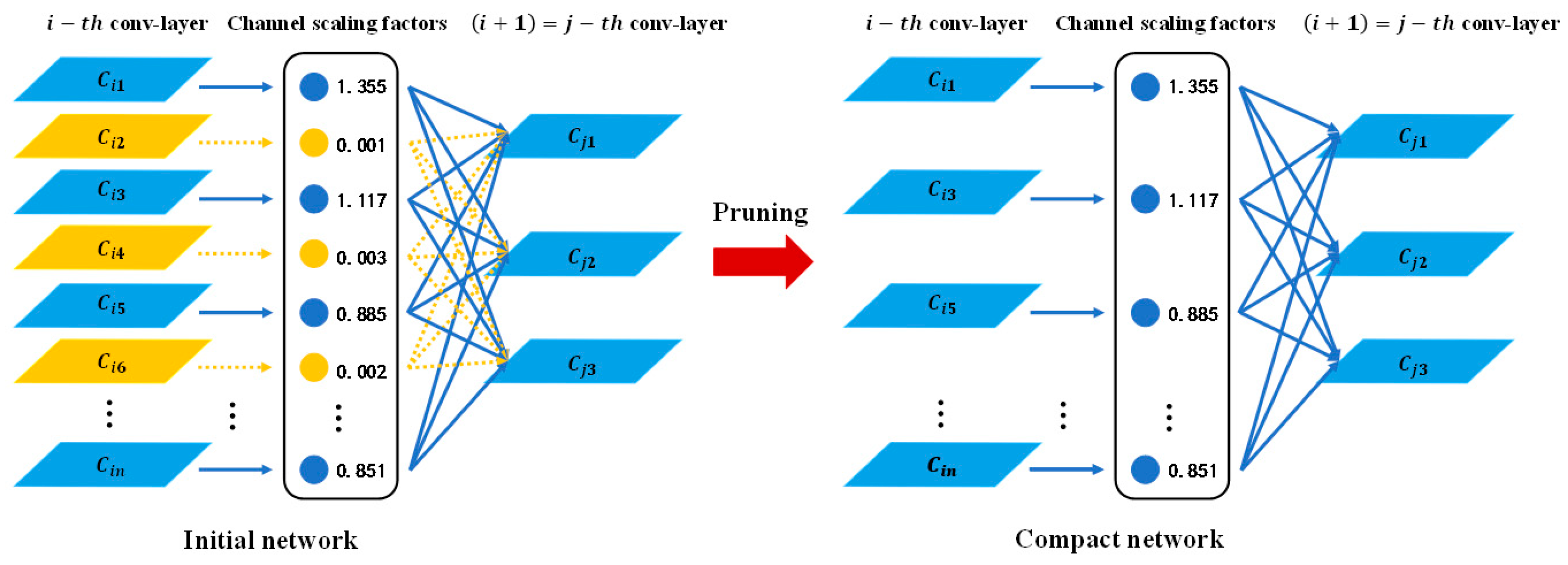
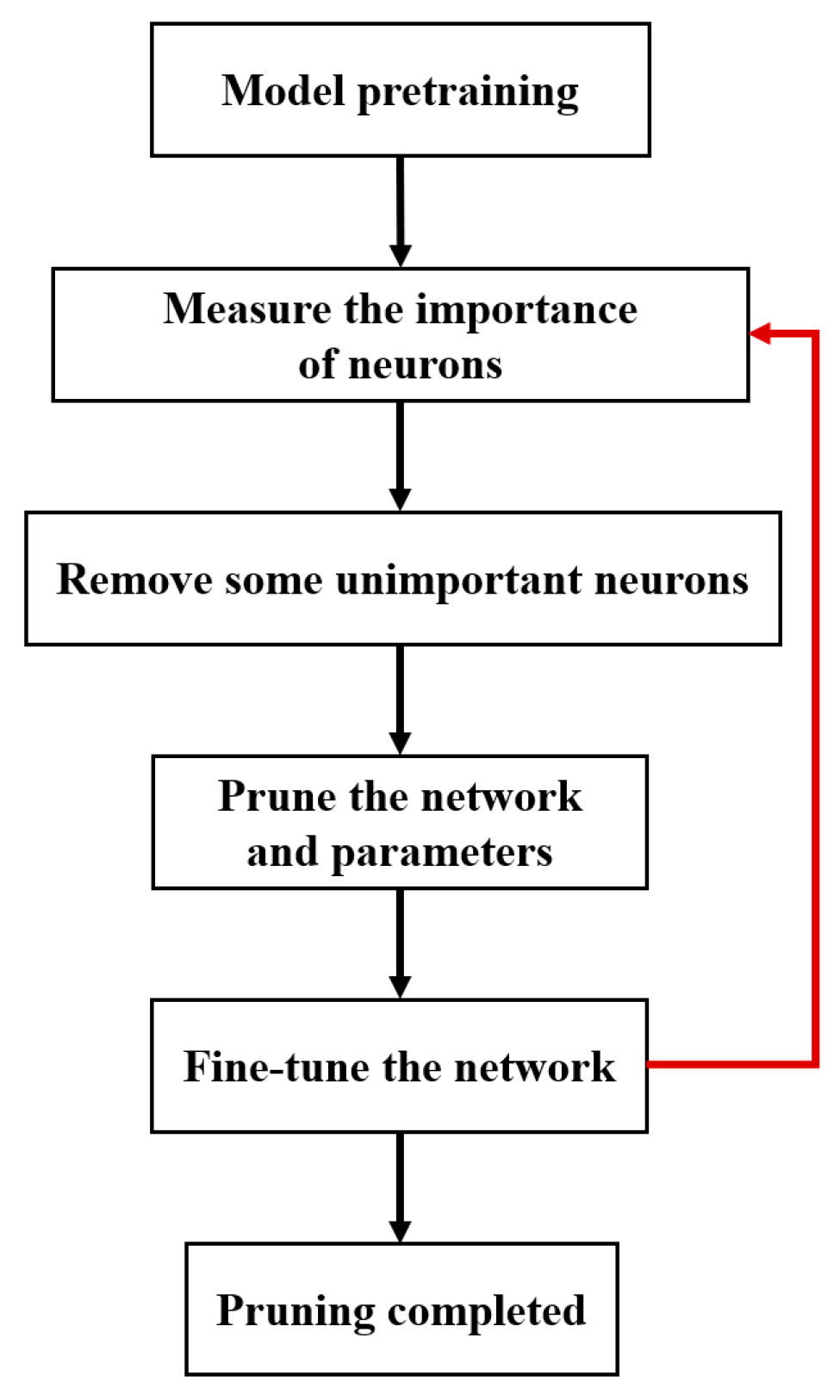
2.2.3. Pruning of the YOLOv4 Workpiece’s Tiny-Surface-Defect Online Detection Model Based on Model Compression Algorithm

Many model compression techniques have been proposed to address the issues of the large model size, memory consumption, and computational load of convolutional neural networks, enabling them to directly learn more efficient models for faster inference [23,24,25]. These methods include low-rank decomposition, network quantization and binarization, weight pruning, dynamic inference, and more. However, these methods often address only one or two of these issues, and some may require specialized software or hardware for acceleration. Another direction for reducing the resource requirements of CNNs is network sparsity, which involves introducing sparsity at various network levels, leading to significant model compression and inference acceleration. However, such methods typically require special software or hardware accelerators to access memory or save time, although this is generally easier to implement than unstructured sparse weight matrices.
In CSP Darknet53, the most significant computations come from the convolutional layers. To reduce the computational load while maintaining the complexity of feature extraction, it is possible to decrease the number of neurons in the convolutional layers, which will correspondingly reduce the number of parameters [26,27,28]. Sparse structures in network models can be implemented at different granularities, including the weight level, kernel level, channel level, and layer level. Fine-grained sparsity offers higher flexibility and generalization capability, resulting in higher compression ratios. However, it often requires the use of software or hardware accelerators for fast inference with sparse models, making it more challenging to implement. Conversely, coarse-grained sparsity does not necessitate special libraries for acceleration and is easier to implement. However, it is less flexible because it may involve pruning entire layers, and it is particularly effective when dealing with very deep neural networks. For coarse-grained pruning, channel pruning strikes a balance between flexibility and implementation ease. It allows for pruning at the filter level, making it more feasible in both software and hardware, achieving a compromise between flexibility and implementation difficulty.
BN layers can normalize the channels, and introducing BN layers can accelerate network training and improve model generalization. In this study, YOLOV4 introduces affine transformation parameters γ and β for the convolutional layers following the BN layer. These affine transformation parameters are iteratively updated through network training, allowing them to learn the feature distribution for each layer. γ , as a scaling factor for channel pruning, is used for network pruning. Its advantage lies in not requiring additional parameters and not adding extra computational burden to the network [29]. The parameter values in the model being close to or becoming zero indicates that they have a minimal impact during neural network propagation. Correspondingly, the neurons associated with such parameters contribute less to the network connections. These less important neurons can be pruned, thus achieving model compression while maintaining overall model detection performance. BN layers use mini-batch data to normalize the internal activation values. Let “ z i n ” and “ z o u t ” represent the input and output of the BN layer, and “B” represents the current mini-batch. The transformation of the BN layer is as shown in the following formula.
z ^ = z i n μ B δ B 2 + ϵ
z o u t = γ z ^ + β
In the equation, “ μ B ” and “ δ B ” represent the mean and standard deviation of the input activations, “ ϵ ” denotes a very small positive value, and “ γ ” and “ β ” represent trainable scaling and shifting parameters, which can linearly transform the normalized values to any scale.
γ ” represents the importance of convolutional filters, with smaller γ values indicating lower importance for the convolutional kernel. Since there are fewer convolutional kernels with γ values close to zero, a sparsity training method is used to train the network weights and the scaling factor γ in the BN layer. This involves introducing L1 regularization and gradually reducing the values of γ during the training process. The objective function trained by this method is as shown in the following formula:
L = ( x , y ) l f x , W , y + λ γ T g ( γ )
In the equation, the first term is the training loss function of the CNN network, where “ ( x , y ) ” represents the training input and target, and “ W ” represents the trainable network weights. The second term is the L1 regularization term on the Gamma coefficients of the BN layer, and g ( · ) applies a sparsity penalty to the scaling factors. λ is the balance factor between the two terms. In the experiments, the selected penalty function for promoting sparsity is the L1 norm, denoted as g s = s , which is used to encourage sparsity.
In the YOLOv4 object detection network, after the convolutional layer operations, the size of the feature map is denoted as w × h × c , where “ w ” and “ h ” represent the width and height of the feature map, and c corresponds to the number of channels in that layer of the network. After processing through a BN layer, you obtain normalized feature maps, and each channel corresponds to a scaling factor γ . After sparse training, the values of the scaling factors γ tend to approach zero or become zero. The total number of statistical parameters γ is counted and sorted. An appropriate pruning ratio is chosen to calculate the maximum γ value that needs to be pruned, denoted as “ s ”. Channels and filters with scaling factors less than or equal to “ s ” are pruned, resulting in the pruned network model. The channel pruning process is detailed in Figure 8.
The algorithm for channel pruning utilizes the Gamma coefficients of the BN layer to assess the contribution scores of input channels. Based on the relationship between distribution coefficients and channel pruning rates, channels with higher contributions (shown in solid blue lines) are retained, while channels with lower contributions (depicted with dashed yellow lines) are removed. In the process of channel connections, neurons in channels with lower contributions do not participate in the connections.
To further compress the model, layer pruning is performed after channel pruning. The layer pruning method employed in this study is derived from the previous channel pruning method. It evaluates the preceding convolution batch normalization mish (CBM) layer for each shortcut layer in the YOLOV4 network, sorts the Gamma means of all layers, and then selects the layer with the lowest mean for pruning. To ensure the integrity of the YOLOV4 structure, when a shortcut structure is pruned, a shortcut layer along with its two preceding convolution layers are simultaneously pruned. The primary focus in this paper is on pruning the shortcut modules in the main network. After completing all pruning operations, the obtained model undergoes fine-tuning to mitigate performance losses resulting from model compression. Pruning operations can be conducted again according to the model’s requirements to meet specific performance criteria. The pruning process is depicted in Figure 9.

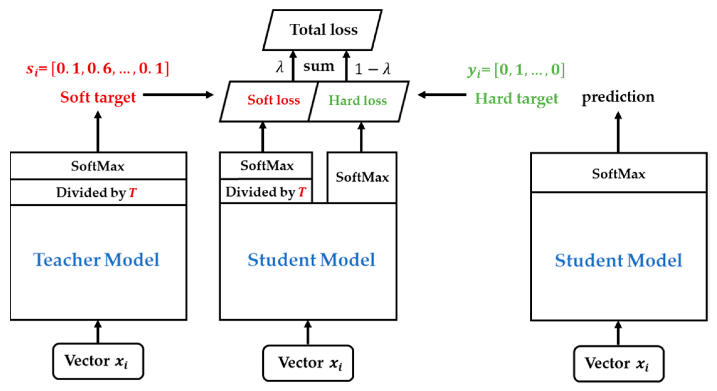
2.2.4. Compression and Post-Processing of the YOLOv4 Workpiece’s Tiny-Surface-Defect Online Detection Model Based on Knowledge Transfer Algorithm

“Knowledge Distillation” is a post-processing method for model compression that enables the transfer of knowledge from a well-trained complex model to a structurally simpler network or allows a simple network to learn from the knowledge of a complex model. The concept of knowledge distillation was initially proposed by Hinton [30] as a compression framework. The basic idea involves introducing a teacher–student network structure, where the soft knowledge from the teacher network model is distilled into the student network model. The teacher network model is obtained through training a deep and wide network for classification or detection tasks, while the student network model is a lightweight model obtained through model compression. This network framework primarily uses soft targets related to the teacher network model as a part of the total loss function to guide the training of the student network model, facilitating the process of knowledge transfer and, thereby, enhancing the accuracy of the compressed model. It employs a SoftMax function with a temperature hyperparameter T to generate predicted probabilities q i for each class, as shown in the following formula:
q i = e x p ( z i T ) j e x p ( z j T )
In the formula, “ q i ” represents the target for the network model to learn (soft target), “ z i ” represents the probability of the i-th class in the network’s output vector, where j 1,2 , 3 , , k , and k is the total number of classes. When T is set to 1, this formula represents the original SoftMax function. When T approaches 0, the maximum value will approach 1, and other values will approach 0, approximating a one-hot encoding. When T is greater than 1, the output distribution becomes smoother, acting as a form of smoothing while retaining similar information. When T is set to infinity, it represents a uniform distribution.
The term “soft target” refers to a target associated with parameter T, aiming to closely resemble the distribution probabilities of the teacher network model with T incorporated. “Hard target,” on the other hand, pertains to the target used in regular network training, with the goal of achieving accurate classification tasks [31]. The student network model involves two loss functions, corresponding to the cross-entropy calculated from soft and hard targets, serving as the loss functions for training the student network model. This enables the student network model to learn features from the teacher network model, resulting in a student network model with fewer parameters and comparable accuracy. During predictions, the trained student network model is used conventionally. Knowledge distillation is a technique that employs a high-performing teacher network model to supervise the training of the student network model, effectively improving the utilization of model parameters.
The structural diagram for knowledge distillation is specifically depicted in Figure 10. The predicted output of the teacher network (on the left-hand side) undergoes a SoftMax calculation after division by the temperature hyperparameter, T, resulting in a softened probability distribution (soft targets or labels) that ranges numerically between 0 and 1, exhibiting a more gradual distribution. A higher value of T leads to a more gradual distribution, while reducing T can amplify the probability of misclassification and introduce unnecessary noise. Hard targets represent the true labels of the samples and can be represented using a one-hot vector. The total loss is designed as the weighted average of the cross-entropy corresponding to both soft and hard targets. A higher weight coefficient for the cross-entropy of soft targets indicates a greater dependency on the contribution of the teacher network during transfer. This is particularly necessary during the initial training stages, aiding the student network in more easily discerning simple samples. However, in the later stages of training, it is essential to appropriately reduce the weight of soft targets, allowing the true labels to aid in distinguishing difficult samples. Additionally, the predictive accuracy of the teacher network is typically superior to that of the student network, and there are no specific constraints on the model’s capacity. Moreover, a higher inference accuracy of the teacher network is more beneficial for the learning process of the student network.
In this study, the value of T is greater than 1, which results in a softened SoftMax, and this soft target can provide more inter-class and intra-class information. For the same input x , the teacher network model and the student network model generate soft targets and soft outputs, respectively. The student network model jointly utilizes soft targets, soft outputs, and hard targets as inputs for the cross-entropy loss function to learn weights, as shown in the following formulas:
P s = s o f t m a x ( z s T )
P t = s o f t m a x ( z t T )
L c l s = λ L s o f t P t , P s + 1 λ L h a r d y , P s
In the equation, “ y ” represents the one-hot encoding of the true labels (hard targets), “ P s ” represents the soft output generated by the student network model, and “ P t ” represents the soft target generated by the teacher network model. “ L c l s ” represents the classification loss, and “ L h a r d ” and “ L s o f t ” represent the classic cross-entropy losses in a classification problem. Due to the use of the soft SoftMax calculation, which involves division by T , the gradient magnitudes associated with soft targets are scaled down by a factor of T 2 . Therefore, it is necessary to consider the factor of T 2 in advance when using λ .
L b R s , R t ,   y = R s y 2 2 , i f   R s y 2 2 + m > R t y 2 2 0 ,                                                             o t h e r w i s e                                                      
L r e g = L s L 1 R s , y r e g + v L b R s , R t ,   y r e g
In the equation, “ L r e g ” represents the regression loss for bounding boxes, “ R s ” represents the regression output of the student network model, “ R t ” represents the regression output of the teacher network model, “ y r e g ” represents the true regression labels, “ m ” represents the margin, “ v ” represents a weight parameter, “ L s L 1 ” represents the absolute loss (smooth L1 loss) function, and “ L b ” represents the bounded regression loss of the teacher network model. The loss function can be computed using the mean absolute error (L1 loss) function, the absolute loss (smooth L1 loss) function, or the mean squared error (L2 loss) function. In this study, the mean squared error (L2 loss) function was used. Using this combination can encourage the student network model to train for regression tasks to be as close as or even better than the teacher network model. When the student network model achieves the same performance as the teacher network model, the teacher network model will not exert excessive influence over the student network model.

2.3. Evaluation of the Model Performance

The commonly used performance evaluation metrics for object detection include mAP and frames per second (FPS). mAP is primarily used to evaluate the accuracy of the model, while FPS is used to assess the model’s speed.
  • mAP
IoU is a highly significant function in the computation of mAP. IoU measures the ratio of the intersection area to the union area between the candidate bound and the ground truth bound. IoU serves as a metric for evaluating the accuracy of object localization in detection. A higher IoU value implies better model performance, indicating greater precision in predictions. The specific calculation formula is as follows:
I o U = a r e a ( B p B g t ) a r e a ( B p B g t )
Electronics 13 00253 i001
Recall (R), also known as sensitivity, is in reference to our original positive samples, indicating how many of the positive samples in the dataset were predicted correctly. After prediction, there are two possibilities for the original positive samples: one is classifying the original positive samples as positive, which we call true positive (TP); the other is classifying the original positive samples as negative, which we refer to as false negative (FN).
R e c a l l = T P T P + F N = T P a l l   g r o u n d   t r u t h s
Using recall values that reflect the classifier’s ability to cover positive samples as the x-axis and precision values that reflect the accuracy of the classifier’s positive predictions as the y-axis, a precision–recall (PR) two-dimensional curve is created, and this PR curve is smoothed. The PR curve demonstrates the trade-off between the classifier’s coverage of positive samples and its precision in correctly identifying them. Average precision (AP) is the area enclosed by the PR curve and the x-axis.
For a continuous PR curve, the specific formula to calculate AP is:
A P = 0 1 P R d r
For a discrete PR curve, the specific formula to calculate AP is:
A P = k = 1 n P ( k ) Δ r ( k )
mAP is the average AP value across all categories, and the specific calculation formula is:
m A P = q = 1 Q A P ( q ) Q
2.
FPS
In object detection algorithms, it is crucial to evaluate not only the accuracy of detection but also an important metric: detection speed. Only with fast detection can real-time online detection be achieved. FPS is used to assess the speed of object detection, indicating the number of images that can be processed per second. A higher FPS value signifies that a greater number of images can be processed per second, indicating a faster detection speed. The specific formula for calculating FPS is:
F P S = f r a m e N u m e l a p s e d T i m e

3. Results and Analysis

This study used an automated production line for a specific aerospace product, which was self-constructed by Guizhou University’s Intelligent Manufacturing Laboratory, as an experimental platform to validate the effectiveness and practicality of the proposed model for the online inspection of workpiece surface quality. In the process of precision machining at the numerical control processing center, workpieces with surface quality below standard may inevitably be produced due to various reasons. Such workpieces, when entering subsequent assembly stages, can easily lead to product rejection, causing delays in production efficiency and resource wastage. The experimental subject of this article is an eccentric conical workpiece. The machining quality at the conical convex platform of this workpiece directly determines the precision in the subsequent assembly stages, making surface quality inspection crucial. The image acquisition facility consists of industrial robots, industrial CCD cameras, industrial lenses, curved LED light sources, and a light-shielding cabinet, as shown in Figure 11. Prior to acquisition, the curved light source is adjusted to the appropriate brightness, lenses are installed on the industrial CCD cameras, and aperture and focal length are adjusted to ensure image quality during acquisition. An industrial robot transports the processed workpieces to the inspection area at a certain speed and triggers the CCD camera to capture images by sending I/O signals. To ensure that the CCD camera captures high-quality images, a precise calibration of the image acquisition facility is required, with hardware models specified as shown in Table 1.
In the experiment, common surface processing defects for the eccentric conical workpiece include “Dent”, “Crack”, “Glitch”, and “Fracture”. A total of 1200 samples of these four defect types were collected during the experiment, with 300 samples for each category. These samples were randomly split, with 80% used as the training dataset and 20% as the testing dataset. The training dataset was used for fitting the data samples and training the relevant parameters. The testing dataset was used for tuning the hyperparameters of the neural network model and evaluating its performance. The training dataset samples were also used for data augmentation, which involves generating additional training samples through various transformations to improve the model’s robustness and generalization.
In the experiment, two different upper-level computer configurations were used to process the data acquired from the image acquisition facility. The former used a high-performance server: the processor was an Intel Xeon Silver 4210 dual-CPU with 20 cores and 40 threads, a clock speed of 2.2 GHz, and a GeForce RTX 2080Ti graphics card with 8 GPUs, each with 11 GB of video memory, and 256 GB of RAM, which was used for training the online surface quality inspection model. The latter utilized Nvidia’s Jetson AGX Xavier developer kit, which consists of a GPU featuring a 512-core NVIDIA Volta™ GPU with 64 Tensor Cores. It was paired with an 8-core ARM 64 v8.2 64-bit CPU, 8 MB L2 + 4 MB L3 cache, 32 GB of 256-bit LPDDR4x memory operating at 137 GB/second, and it had a 32 GB eMMC 5.1 storage. This setup is designed for deploying lightweight deep learning models in industrial scenarios. This configuration was utilized for the deployment of a pruned workpiece-surface-quality online inspection model in an industrial setting. The software platform used was the Ubuntu 18.04 LTS operating system, and the deep learning model framework employed was PyTorch (v 2.0). The detection model selects nine different sizes of anchor boxes using the K-means++ clustering method, and these anchor box sizes are then separately applied to the three branches of the feature pyramid network. In the case of the deeper feature maps, specifically the outputs of Residual Block1 and Residual Block2, three anchor box sizes are used, which correspond to the smallest and medium-sized areas. For the shallower feature map, which is the output of Residual Block3, three anchor box sizes with the largest areas are employed. Furthermore, the learning rate in this study was initially set to 0.001 and underwent exponential decay as the number of iterations increased. Pretrained model weights that have undergone extensive training on the ImageNet dataset were used as the initial weights for the feature extraction network. Specific model training parameters are outlined in Table 2.

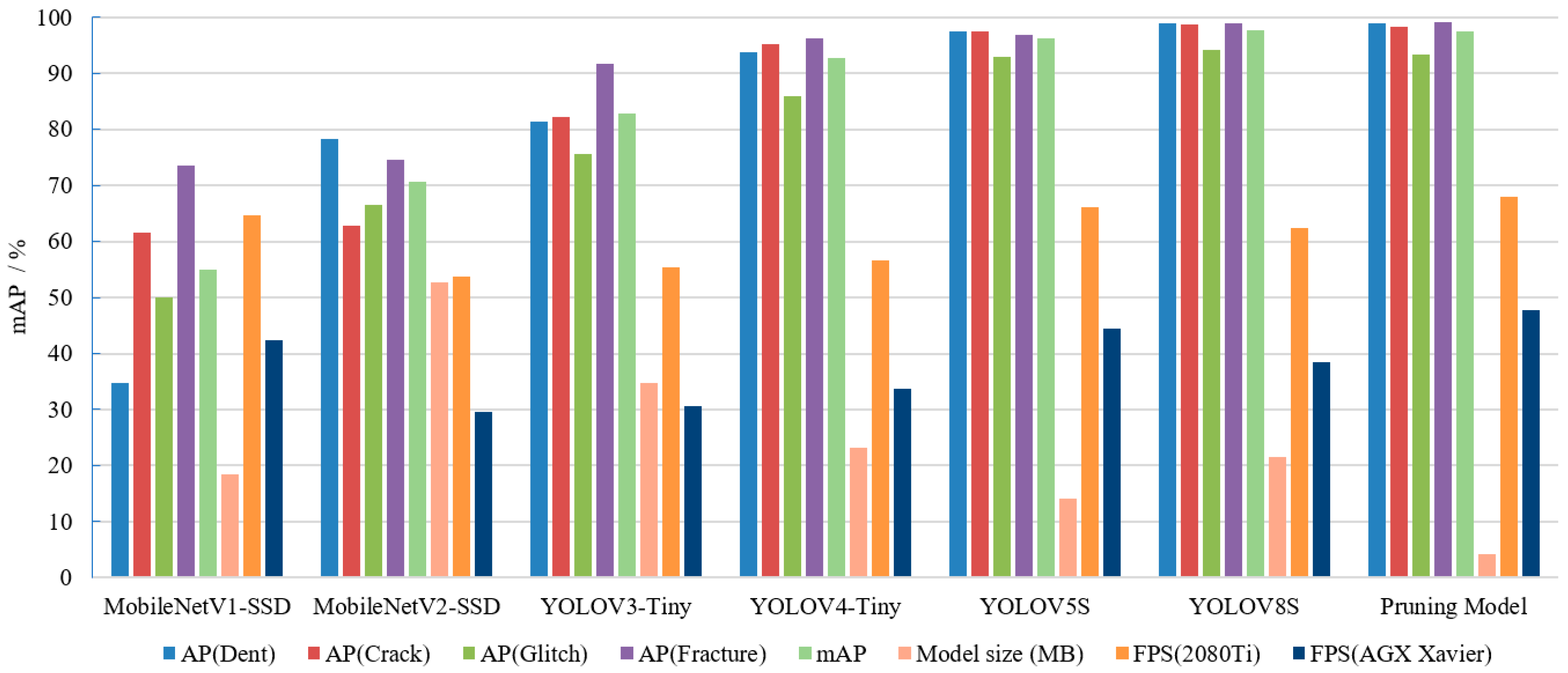
3.1. Comparison of Different Object Detection Algorithms

The product-surface-quality online inspection model designed in this study employs the CutMix data augmentation method and the K-means++ clustering method in the sample preprocessing stage to improve the algorithm’s robustness. This allows the generated anchor boxes to select more fine-grained features at an earlier stage. The training process of the surface quality online inspection model is shown in detail in Figure 11, while the training process of the YOLOV4-tiny model is specified in Figure 12. Model performance is evaluated on the test set using mAP as a metric every 15 epochs.
In the early stages of model training for the workpiece-surface-quality online inspection model, the learning rate was set relatively high, and the training curve converged quickly. As training progressed, the slope of the training curve gradually decreased. Finally, when the number of training iterations reached 150 epochs, the model’s learning efficiency was gradually saturated, and the loss fluctuated around 0.27.
As shown in Figure 12 and Figure 13, both models converged rapidly. The surface quality online inspection model and YOLOV4-tiny model reached an accuracy of over 90.00% after approximately 55 epochs and 130 epochs of training, respectively. Meanwhile, under the evaluation with an IoU threshold of 0.5, the former achieved a final mAP of 97.50%, while the latter reached 92.74%. It is evident that the surface quality online inspection model designed for industrial products with stable shapes, singularity, and small variation in defect size exhibited advantages in terms of convergence performance and detection performance. This study further investigated the performance of these models and other object detection models in subsequent experiments.
Deep learning methods have achieved significant success in the field of object detection, surpassing traditional algorithms in both accuracy and robustness. One-stage detection models, which balance real-time performance and accuracy, are particularly suitable for engineering applications. The experiments use the versatile YOLO series and SSD as the detection substructures, combined with DarkNet-53 [11], InceptionV2 [32], and InceptionV3 [33] for comparative tests. Specifically, SSD-InceptionV2, SSD-InceptionV3, YOLOV3, and YOLOV4-tiny are used as comparison models. Since mAP is the most widely used comprehensive evaluation metric in object detection tasks, the experiments follow the evaluation approach used in the COCO dataset [34] with an IoU threshold of 0.5. This approach takes into account both localization and recognition accuracy and deeply explores the differences in the models’ capabilities in detection tasks. The specific experimental results are shown in Table 3.
From Table 3, it can be observed that the workpiece surface quality online inspection model has achieved quite satisfactory results. During validation on the test set, this model is capable of finely learning high-quality features, accurately identifying types of defects within the samples, and generating detection results highly similar to the real bounding boxes. During testing, the surface quality online inspection model achieved an FPS score of 32.8 f/s on a single GeForce RTX 2080Ti card. While it may not outperform other detection models in terms of FPS, it still meets the real-time requirements of the industrial field, especially in scenarios with adequate hardware resources.

3.2. Comparison of the Proposed Method with Previous Studies

While the improved surface quality online inspection model can effectively detect the machining quality of workpiece surfaces, the YOLOV4 network has a large number of model parameters, and its deep network structure results in significant computational demands. To reduce the model’s parameters and complexity, decrease its resource requirements, and make it deployable on edge computing devices with limited computational capabilities, channel pruning is employed. Channel pruning fundamentally involves the identification and elimination of unimportant channels within the network, along with their associated input and output relationships, thereby reducing the number of parameters that need to be stored. In addition, layer pruning is performed on top of channel pruning to further decrease the computational load, enhance the model’s inference speed, and achieve compression in both the width and depth of the network. Consequently, this paper employs both channel pruning and layer pruning methods to trim the trained workpiece-surface-quality online inspection model, ultimately striking a balance between flexibility and implementation cost.
The specific steps of the model compression method in this research include the following:
1.
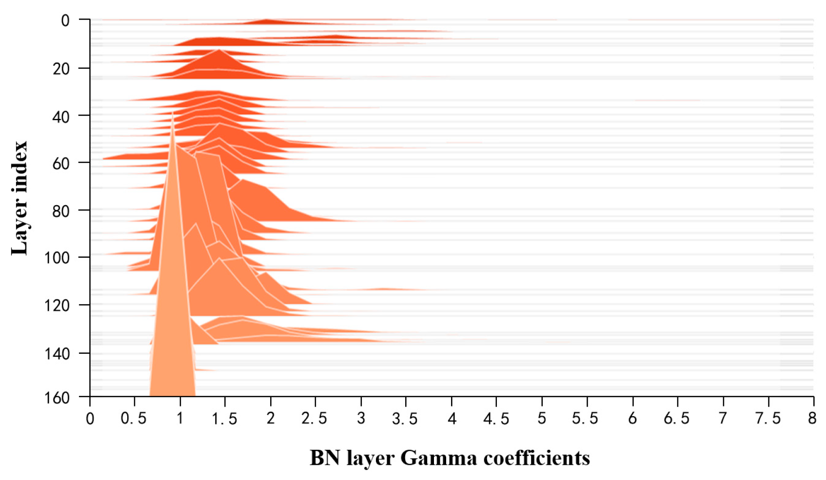
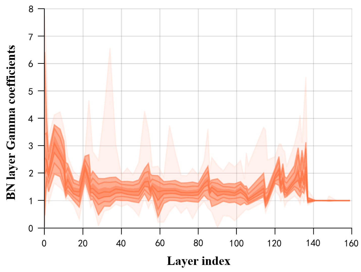
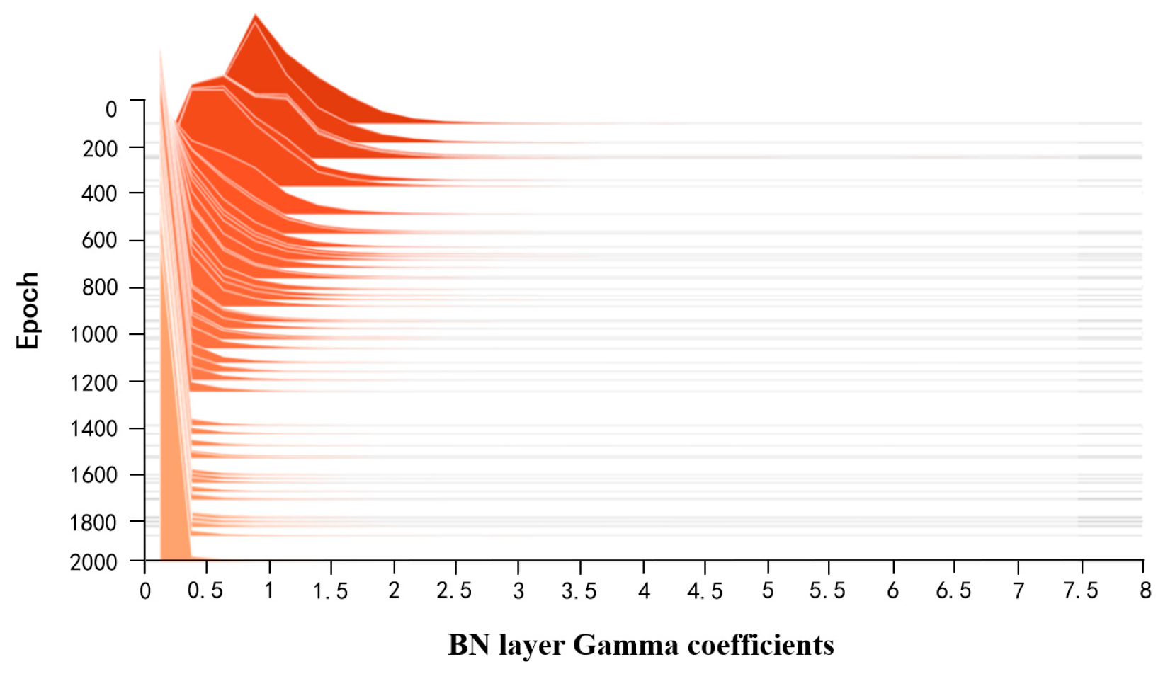
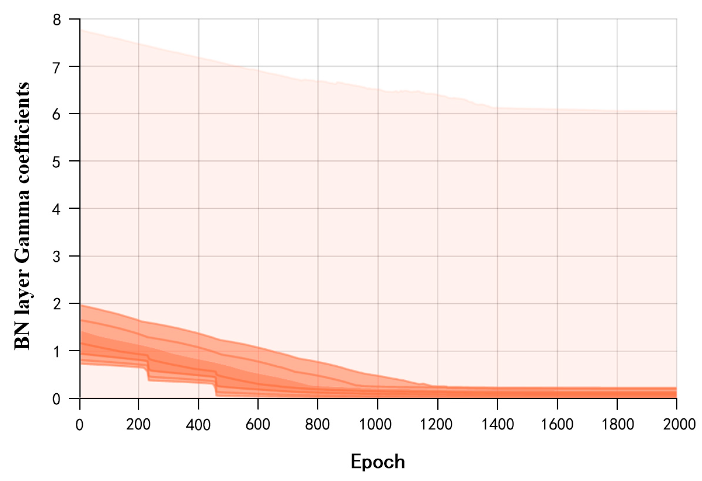
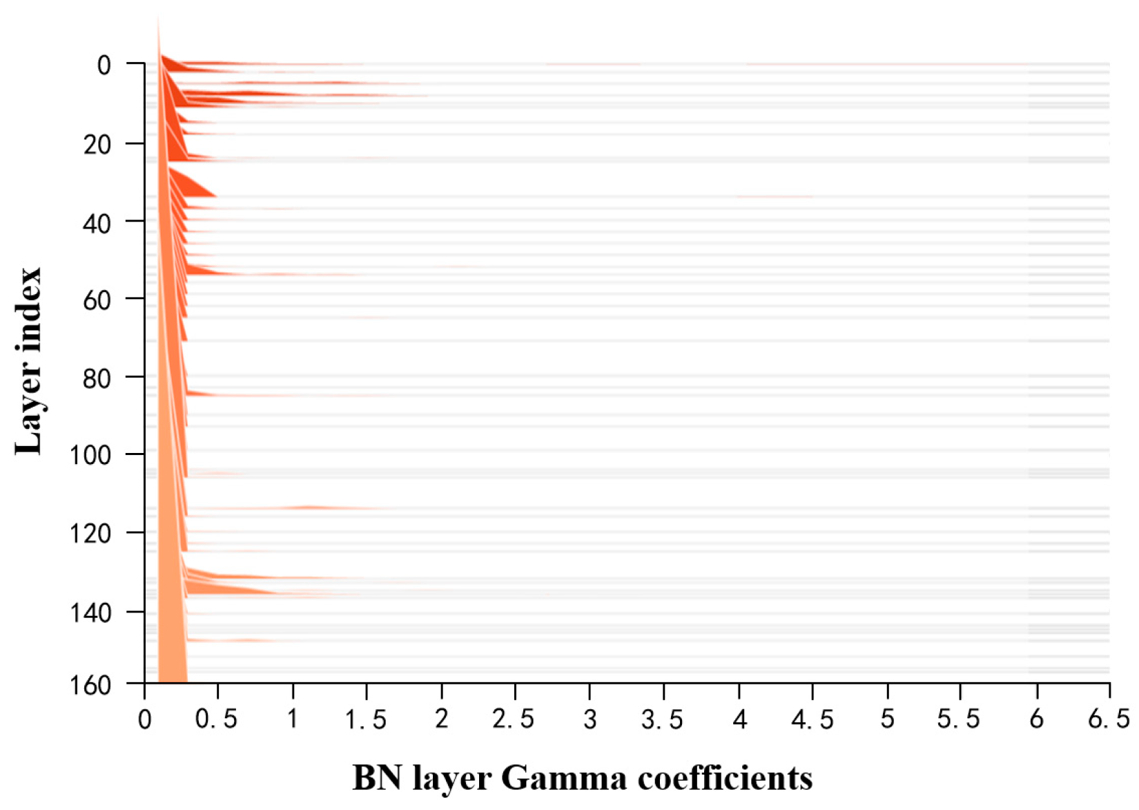
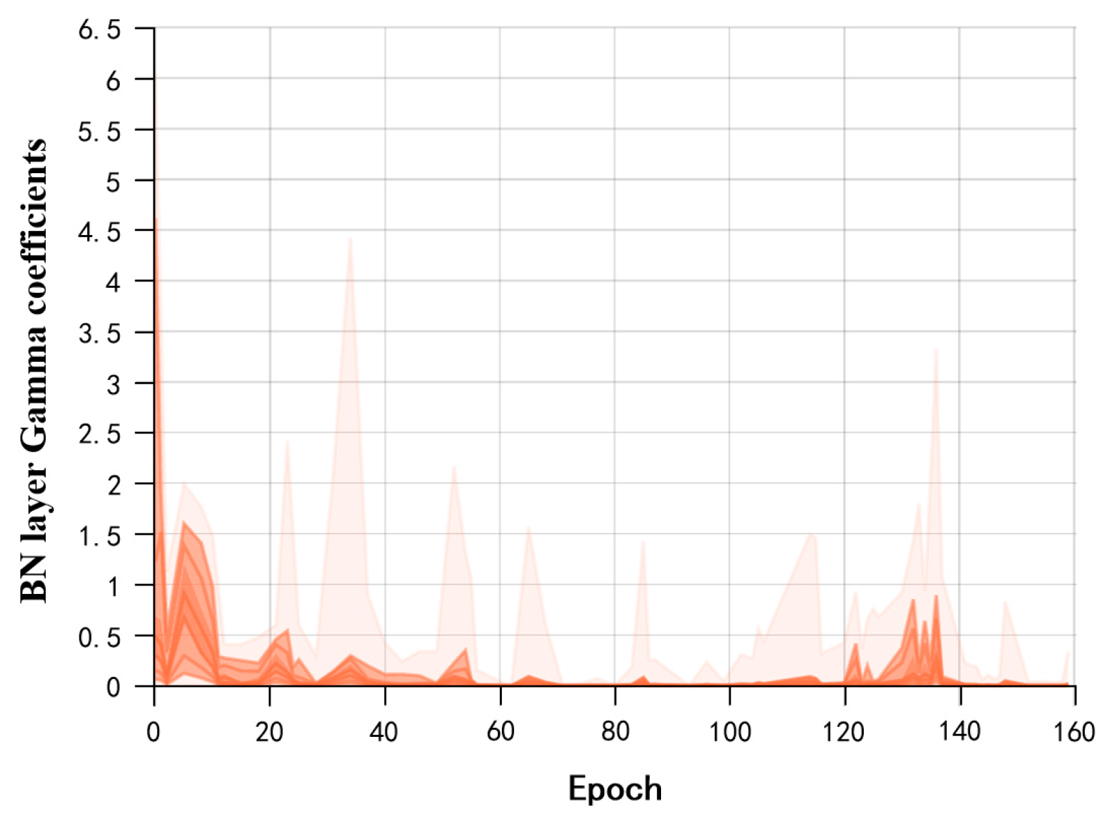
Sparse Training: Apply L1 regularization constraints to the coefficients of the BN layers in the surface-quality online inspection model to adjust the sparsity of the model in the structural direction.
2.
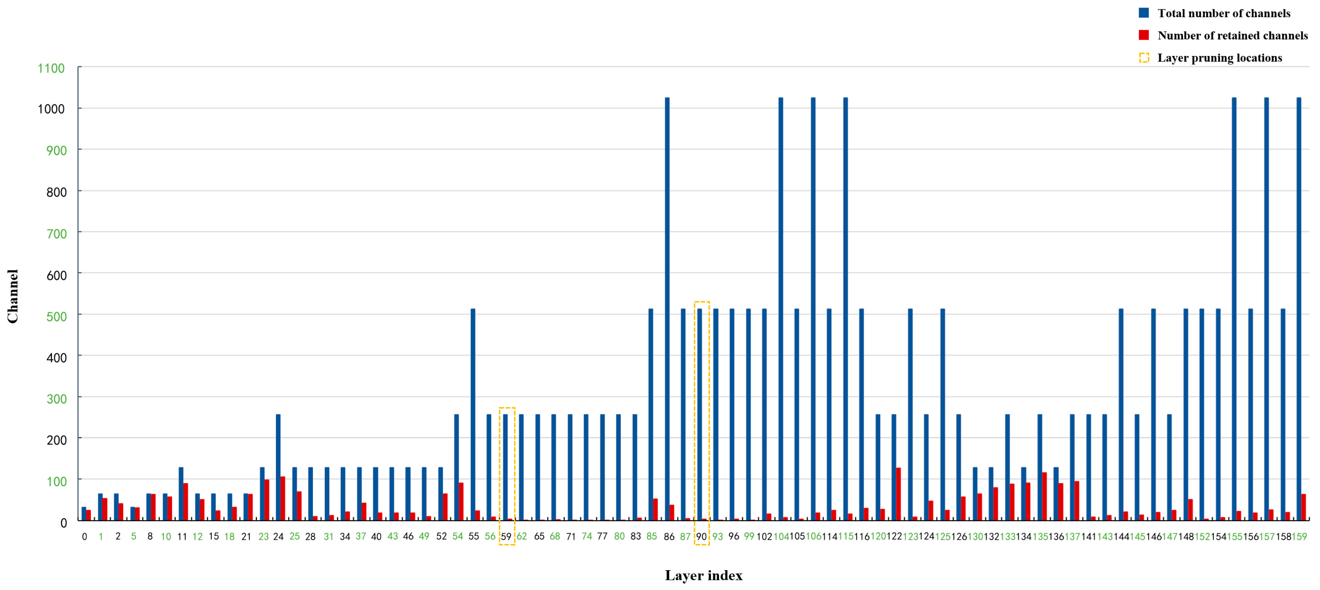
Pruning: After sparse training, perform channel pruning and layer pruning on the sparse model according to a certain pruning ratio to generate a compact model, reducing its storage space requirements.
3.
Fine-tuning the Pruned Model: The primary purpose is to overcome the issue of excessive loss of accuracy after model pruning. Knowledge distillation is used to effectively recover the lost accuracy. The specific parameters for model compression are outlined in Table 4.
These steps collectively contribute to reducing the model’s size while maintaining its performance, allowing for deployment on resource-constrained edge computing devices.
Sparse training is essentially a trade-off between model accuracy and sparsity. Different sparse strategies need to be applied for different models to achieve a high sparsity while maintaining a high accuracy. Generally, choosing a larger sparsity rate can accelerate the model’s sparsity but result in a faster drop in accuracy. On the other hand, selecting a smaller sparsity rate, although slower in sparsity reduction, also leads to a slower decrease in accuracy. Additionally, combining a larger learning rate can speed up the sparsity process, while using a smaller learning rate later helps the accuracy recover. After multiple experiments, this study ultimately chose a constant-sparsity strategy for sparse training. This means that throughout the entire sparsity process, a constant sparsity rate is used to add extra gradients to the model. This approach provides a relatively even force, resulting in higher compression levels. The specific distribution and values of the Gamma coefficients of the BN layers before sparse training are shown in Figure 14 and Figure 15.
The specific distribution and coefficient changes of the Gamma coefficients of the BN layers during sparse training are shown in Figure 16 and Figure 17. During the sparse training process, with an increasing number of iterations, the center of the Gamma coefficient distribution for all BN layers gradually moves in the direction of 0. However, not all BN layers’ Gamma coefficients decay to 0, indicating that the Gamma coefficients are gradually becoming sparse. After about 1800 iterations of sparse training, there is only a slight change in the sparsity of the Gamma coefficients, suggesting that sparse training has reached saturation. The specific distribution and values of the Gamma coefficients of the BN layers after sparse training are depicted in Figure 18 and Figure 19.
After sparse training, a channel pruning ratio of 0.90 was applied to prune the workpiece-surface-quality online inspection model. Since YOLOV4 includes five sets of 23 shortcut layer connections with corresponding “add” operations, and to ensure that the two input dimensions of the shortcut layers remain consistent after channel pruning, layers directly connected to the shortcut layers were not pruned. This helped avoid dimension issues while effectively reducing model parameters to achieve a higher pruning ratio. The specific changes in the number of channels for each layer before and after pruning are shown in Figure 20. After pruning, the channel count ranged from 1 to 127 channels, with a maximum pruning of 1017 channels and a minimum pruning of 1 channel. Subsequently, layer pruning was performed after channel pruning. For layer pruning, each preceding CBM layer for each shortcut layer was evaluated. The layers were sorted based on the mean Gamma values, and the layers with the smallest mean Gamma values were selected for layer pruning. According to the sorting results, this study selected layer 59 and layer 90 for pruning. Table 5 presents the test results after model compression. After channel pruning, the model’s parameter count was reduced by 98.27%, the model size was reduced by 98.24%, and the average accuracy mean was decreased by 2.36%. After layer pruning, the model’s parameter count was reduced by 98.31%, the model size was reduced by 98.28%, and the average accuracy mean was decreased by 2.36%, which is consistent with the results after channel pruning.
After model compression, there is usually a decrease in accuracy, and it is necessary to fine-tune the compressed model to restore its accuracy. This study employed both knowledge distillation and non-knowledge distillation methods to train the compressed surface-quality online inspection model. As shown in Figure 21, when the non-knowledge distillation method is used, after 100 iterations, the model achieves an optimal accuracy of 96.05%, which is 1.29% lower than the accuracy of the uncompressed model. As shown in Figure 22, when knowledge distillation is employed for fine-tuning, after 90 iterations, the model’s accuracy reaches 97.41%, which is almost consistent with the accuracy of the uncompressed model. The experimental results demonstrate that model compression can effectively simplify the model while ensuring the accuracy of the workpiece-surface-quality online inspection model.
This study compared the fine-tuned compressed model with classic lightweight object detection models such as MobileNetV1-SSD [35], MobileNetV2-SSD [36], YOLOV3-Tiny [11], YOLOV4-Tiny [12], YOLOV5S [13,37], and YOLOV8S [14,38] on the test set, as shown in Table 6. From the table, it is evident that the pruned surface quality online detection model achieved relatively excellent performance compared to several other lightweight deep learning models. It reached a detection accuracy of 97.41%, which is essentially consistent with the YOLOV8S model’s accuracy. However, the model’s size reduced by 80.51% compared to YOLOV8S, and its detection speed is superior to YOLOV8S. The pruned surface-quality online detection model achieved a good balance between accuracy and speed. Furthermore, due to the removal of a significant number of convolution channels, the model’s parameter count was greatly reduced. During the experiments, the pruned model achieved an FPS of 47.8 when tested using the Jetson AGX Xavier development kit with the validation test set images, enabling deployment in industrial scenarios with limited hardware resources. The specific detection results for the product-surface-quality online inspection model before and after improvement are presented in Figure 23. It can be observed from Table 6 and Figure 24 that the improved product-surface-quality online inspection model still maintains the same level of detection accuracy as the model before improvement.

4. Conclusions

This study primarily focused on constructing a rule-based digital twin model for the surface quality inspection of in-process products. It proposed an improved product-surface-quality online inspection model based on model compression, which is designed for deployment on edge computing devices to identify and label minor defects on product surfaces, thereby providing the foundation for building macro-level automated-manufacturing-process digital twin models. Firstly, in the preprocessing stage, the study introduced the use of mosaic data augmentation methods to enhance the diversity of training samples, improve the model’s robustness and generalization, and avoid overfitting. It also employed the K-means++ clustering algorithm to generate anchor boxes, adapting to different defect sizes and selecting finer features earlier in the process. Secondly, it utilized the CSP Darknet53 network and the SPP module to extract features from the input raw images. Through training, it developed an online detection model tailored to workpiece-surface-quality, thereby improving the accuracy of defect localization and recognition in YOLOV4. Finally, the study integrated the concept of model compression by incorporating sparse training into the model using scaling factors in BN layers. It applied sparse factors to the network, performed channel pruning and layer pruning on the sparse model, and employed knowledge distillation methods. This approach effectively reduced the model’s size and forward inference time while maintaining the model’s accuracy. It is beneficial for deploying network models on edge computing devices with limited GPU and storage resources.
Experimental results demonstrated that the proposed method for improving deep convolutional neural networks through model compression can compress the model size from 244 M to 4.19 M, achieving a prediction accuracy of 97.41% and a detection speed of 47.8 f/s (AGX Xavier test results). These results outperform similar deep learning algorithms, making the method suitable for use in rule-based models for product-surface-quality inspection via digital twins. This allows for an accurate representation and a synchronous mapping of the current quality status of in-process products. The effectiveness of this approach was validated through in-process product-surface-quality online inspection on an aerospace product automated production line.
Based on this research, the following needs are identified for future research:
1.
The study focused extensively on the combination of the YOLO network, model compression, and knowledge distillation algorithms. With the continuous development of object detection networks, future research will incorporate different attention mechanisms to improve network models, achieving better detection performance and lighter models.
2.
The limited quantity of defect samples that the study could collect may be enhanced in the future by considering effective data augmentation using generative adversarial networks (GANs) on original samples. This approach generates new samples with different characteristics from the original data but possessing similar features, thereby enhancing the algorithm’s robustness.
3.
The algorithm employed in the study belongs to supervised learning. Acquiring a large volume of annotated data in industrial sectors is challenging and requires substantial human resources. Therefore, focusing on how to apply unsupervised learning techniques to practical defect detection tasks will be a key area of future research direction.

Author Contributions

Conceptualization, Q.C.; methodology, Q.C. and Q.X.; software, Q.C.; validation, Q.C. and Q.X.; formal analysis, Q.C.; investigation, Q.C.; resources, Q.C. and Z.L.; data curation, Q.C.; writing—original draft preparation, Q.C.; writing—review and editing, Q.C.; visualization, Q.C.; supervision, H.H. and S.T.; project administration, Q.C. and H.H.; funding acquisition, Q.C. and Z.L. All authors have read and agreed to the published version of the manuscript.

Funding

This research was funded by the Open Fund Project supported by the Key Laboratory of Advanced Manufacturing Technology Ministry of Education, China (Grant No. QJH KY [2022]377), Guizhou Provincial Basic Research Program (Natural Science) (Grant No. Qiankehejichu-ZK [2023] General 014), Growth Project for Young Scientific and Technological Talents in General Colleges and Universities of Guizhou Province (Grant No. Qianjiaoji [2022]303), Introducing Talents to Initiate Funded Research Projects of Guiyang University (Grant No. GYU-KY-[2024]), Guizhou Provincial Department of Education Science and Technology Top Talent Program (Grant No. [2022]086), and Guiyang City Science and Technology Plan Program (Grant No. [2023]48-18).

Institutional Review Board Statement

Not applicable.

Informed Consent Statement

Not applicable.

Data Availability Statement

Data are contained within the article.

Conflicts of Interest

The authors declare no conflict of interest.

Abbreviations

CSPCross Stage Partial
SPPSpatial Pyramid Pooling
BNBatch Normalization
HOGHistogram of Oriented Gradient
LBPLocal Binary Pattern
SVMSupport Vector Machine
RBFRadial Basis Function
CNNConvolutional Neural Networks
R-CNNRegion-based Convolutional Neural Network
YOLOYou Only Look Once
SSDSingle Shot Multibox Detector
GAGenetic Algorithm
mAPMean Average Precision
DRDefect Recognition
DSCDepthwise Separable Convolution
HPFRCCsHigh-performance Fiber-reinforced Cementitious Composites
CCDCharge Coupled Device
IoUIntersection over Union
FPNFeature Pyramid Network
PANPath Aggregation Network
CBMConvolution Batch Normalization Mish
FPSFrames per Second
RRecall
TPTrue Positive
FNFalse Negative
PRPrecision-Recall
APAverage Precision
GANsGenerative Adversarial Networks

References

  1. Tulbure, A.A.; Tulbure, A.A.; Dulf, E.H. A review on modern defect detection models using DCNNs–Deep convolutional neural networks. J. Adv. Res. 2022, 35, 33–48. [Google Scholar] [CrossRef] [PubMed]
  2. Chen, Y.; Ding, Y.; Zhao, F.; Zhang, E.; Wu, Z.; Shao, L. Surface defect detection methods for industrial products: A review. Appl. Sci. 2021, 11, 7657. [Google Scholar] [CrossRef]
  3. Ren, Z.; Fang, F.; Yan, N.; Wu, J. State of the art in defect detection based on machine vision. Int. J. Precis. Eng. Manuf.-Green Technol. 2022, 9, 661–691. [Google Scholar] [CrossRef]
  4. Liu, L.; Wang, C.; Zhao, S.; Li, H. Research on solar cells defect detection technology based on machine vision. J. Electron. Meas. Instrum. 2018, 32, 47–52. [Google Scholar]
  5. Song, W.; Zuo, D.; Deng, B.; Zhang, H. Corrosion defect detection of earthquake hammer for high voltage transmission line. Chin. J. Sci. Instrum. 2016, 37, 113–117. [Google Scholar]
  6. Ge, Q.; Fang, M.; Xu, J. Defect Detection of Industrial Products based on Improved Hough Transform. In Proceedings of the 2018 IEEE International Conference on Mechatronics and Automation (ICMA), Changchun, China, 5–8 August 2018; pp. 832–836. [Google Scholar] [CrossRef]
  7. Ding, S.; Liu, Z.; Li, C. AdaBoost learning for fabric defect detection based on HOG and SVM. In Proceedings of the IEEE 2011 International Conference on Multimedia Technology, Hangzhou, China, 26–28 July 2011. [Google Scholar]
  8. Girshick, R.; Donahue, J.; Darrell, T.; Malik, J. Rich feature hierarchies for accurate object detection and semantic segmentation. In Proceedings of the IEEE Conference on Computer Vision and Pattern Recognition, Columbus, OH, USA, 23–28 June 2014; pp. 580–587. [Google Scholar]
  9. Redmon, J.; Divvala, S.; Girshick, R.; Farhadi, A. You only look once: Unified, real-time object detection. In Proceedings of the IEEE Conference on Computer Vision and Pattern Recognition, Las Vegas, NV, USA, 27–30 June 2016; pp. 779–788. [Google Scholar]
  10. Redmon, J.; Farhadi, A. YOLO9000: Better, faster, stronger. In Proceedings of the IEEE Conference on Computer Vision and Pattern Recognition, Honolulu, HI, USA, 21–26 July 2017; pp. 7263–7271. [Google Scholar]
  11. Redmon, J.; Farhadi, A. Yolov3: An incremental improvement. arXiv 2018, arXiv:1804.02767. [Google Scholar]
  12. Bochkovskiy, A.; Wang, C.Y.; Liao HY, M. Yolov4: Optimal speed and accuracy of object detection. arXiv 2020, arXiv:2004.10934. [Google Scholar]
  13. Jocher, G.; Stoken, A.; Borovec, J.; Stan, C.; Changyu, L.; Rai, P.; Ferriday, R.; Sullivan, T.; Xinyu, W.; Ribeiro, Y.; et al. Ultralytics/yolov5: v3. 0; Zenodo: Zurich, Switzerland, 2020. [Google Scholar]
  14. Li, C.; Li, L.; Jiang, H.; Weng, K.; Geng, Y.; Li, L.; Ke, Z.; Li, Q.; Cheng, M.; Nie, W.; et al. YOLOv6: A single-stage object detection framework for industrial applications. arXiv 2022, arXiv:2209.02976. [Google Scholar]
  15. Wang, C.Y.; Bochkovskiy, A.; Liao HY, M. YOLOv7: Trainable bag-of-freebies sets new state-of-the-art for real-time object detectors. In Proceedings of the IEEE/CVF Conference on Computer Vision and Pattern Recognition, Vancouver, BC, Canada, 17–24 June 2023; pp. 7464–7475. [Google Scholar]
  16. Contributors, M. YOLOv8 by MMYOLO. 2023. Available online: https://github.com/open-mmlab/mmyolo/tree/main/configs/yolov8 (accessed on 13 May 2023).
  17. Liu, W.; Anguelov, D.; Erhan, D.; Szegedy, C.; Reed, S.; Fu, C.-Y.; Berg, A.C. Ssd: Single shot multibox detector. In Proceedings of the Computer Vision–ECCV 2016: 14th European Conference, Part I 14, Amsterdam, The Netherlands, 11–14 October 2016; Springer International Publishing: Berlin/Heidelberg, Germany, 2016; pp. 21–37. [Google Scholar]
  18. Chen, M.; Yu, L.; Zhi, C.; Sun, R.; Zhu, S.; Gao, Z.; Ke, Z.; Zhu, M.; Zhang, Y. Improved faster R-CNN for fabric defect detection based on Gabor filter with Genetic Algorithm optimization. Comput. Ind. 2022, 134, 103551. [Google Scholar] [CrossRef]
  19. Duan, L.; Yang, K.; Ruan, L. Research on automatic recognition of casting defects based on deep learning. IEEE Access 2020, 9, 12209–12216. [Google Scholar] [CrossRef]
  20. Zhou, Z.; Zhang, J.; Gong, C. Automatic detection method of tunnel lining multi-defects via an enhanced You Only Look Once network. Comput. Aided Civ. Infrastruct. Eng. 2022, 37, 762–780. [Google Scholar] [CrossRef]
  21. Li, Y.; Huang, H.; Xie, Q.; Yao, L.; Chen, Q. Research on a surface defect detection algorithm based on MobileNet-SSD. Appl. Sci. 2018, 8, 1678. [Google Scholar] [CrossRef]
  22. Guo, P.; Meng, W.; Bao, Y. Automatic identification and quantification of dense microcracks in high-performance fiber-reinforced cementitious composites through deep learning-based computer vision. Cem. Concr. Res. 2021, 148, 106532. [Google Scholar] [CrossRef]
  23. Wu, D.; Lv, S.; Jiang, M.; Song, H. Using channel pruning-based YOLOv4 deep learning algorithm for the real-time and accurate detection of apple flowers in natural environments. Comput. Electron. Agric. 2020, 178, 105742. [Google Scholar] [CrossRef]
  24. Geng, L.; Niu, B. A Survey of Deep Neural Network Model Compression. J. Front. Comput. Sci. Technol. 2020, 14, 1441–1455. [Google Scholar]
  25. Tan, X.; Wang, Z. Ping pong ball recognition using an improved algorithm based on YOLOv4. Technol. Innov. Appl. 2020, 27, 74–76. [Google Scholar]
  26. Zhou, J.; Jing, J.; Zhang, H.; Wanh, Z.; Huang, H. Real-time fabric defect detection algorithm based on S-YOLOV3 model. Laser Optoelectron. Prog. 2020, 57, 55–63. [Google Scholar]
  27. Zhang, Y.; Wu, J.; Ma, Z.; Cao, X.; Guo, W. Compression and implementation of neural network model base on YOLOv3. Micro/Nano Electron. Intell. Manuf. 2020, 178, 105742. [Google Scholar]
  28. Bai, S. Research on Traffic Signs Detection and Recognition Algorithm Base on Deep Learning. Ph.D. Thesis, Changchun University of Technology, Changchun, China, 2020; p. 159. [Google Scholar]
  29. Liu, Z.; Li, J.; Shen, Z.; Huang, G.; Yan, S.; Zhang, C. Learning efficient convolutional networks through network slimming. In Proceedings of the IEEE International Conference on Computer Vision, Venice, Italy, 22–29 October 2017; pp. 736–2744. [Google Scholar]
  30. Hinton, G.; Vinyals, O.; Dean, J. Distilling the knowledge in a neural network. arXiv 2015, arXiv:1503.02531. [Google Scholar]
  31. Chen, G.; Choi, W.; Yu, X.; Han, T.; Chandraker, M. Learning efficient object detection models with knowledge distillation. Adv. Neural Inf. Process. Syst. 2017, 30, 1–10. [Google Scholar]
  32. Ioffe, S.; Szegedy, C. Batch normalization: Accelerating deep network training by reducing internal covariate shift. In Proceedings of the International Conference on Machine Learning—PMLR, Lille, France, 6–11 July 2015; pp. 448–456. [Google Scholar]
  33. Szegedy, C.; Vanhoucke, V.; Ioffe, S.; Shlens, J.; Wojna, Z. Rethinking the inception architecture for computer vision. In Proceedings of the IEEE 32nd Conference on Computer Vision and Pattern Recognition, Las Vegas, NV, USA, 27–30 June 2016; pp. 2818–2826. [Google Scholar]
  34. Lin, T.Y.; Maire, M.; Belongie, S.; Hays, J.; Perona, P.; Ramanan, D.; Dollár, P. Microsoft coco: Common objects in context. In Proceedings of the Computer Vision–ECCV 2014: 13th European Conference, Part V 13, Zurich, Switzerland, 6–12 September 2014; Springer International Publishing: Berlin/Heidelberg, Germany, 2014; pp. 740–755. [Google Scholar]
  35. Howard, A.G.; Zhu, M.; Chen, B.; Kalenichenko, D.; Wang, W.; Weyand, T.; Andreetto, M.; Adam, H. Mobilenets: Efficient convolutional neural networks for mobile vision applications. arXiv 2017, arXiv:1704.04861. [Google Scholar]
  36. Howard, A.; Zhmoginov, A.; Chen, L.C.; Sandler, M.; Zhu, M. Inverted residuals and linear bottlenecks: Mobile networks for classification, detection and segmentation. In Proceedings of the IEEE Conference on Computer Vision and Pattern Recognition (CVPR), Salt Lake City, UT, USA, 18–23 June 2018. [Google Scholar]
  37. Guo, P.; Meng, X.; Meng, W.; Bao, Y. Monitoring and automatic characterization of cracks in strain-hardening cementitious composite (SHCC) through intelligent interpretation of photos. Compos. Part B Eng. 2022, 242, 110096. [Google Scholar] [CrossRef]
  38. Li, Y.; Fan, Q.; Huang, H.; Han, Z.; Gu, Q. A Modified YOLOv8 Detection Network for UAV Aerial Image Recognition. Drones 2023, 7, 304. [Google Scholar] [CrossRef]
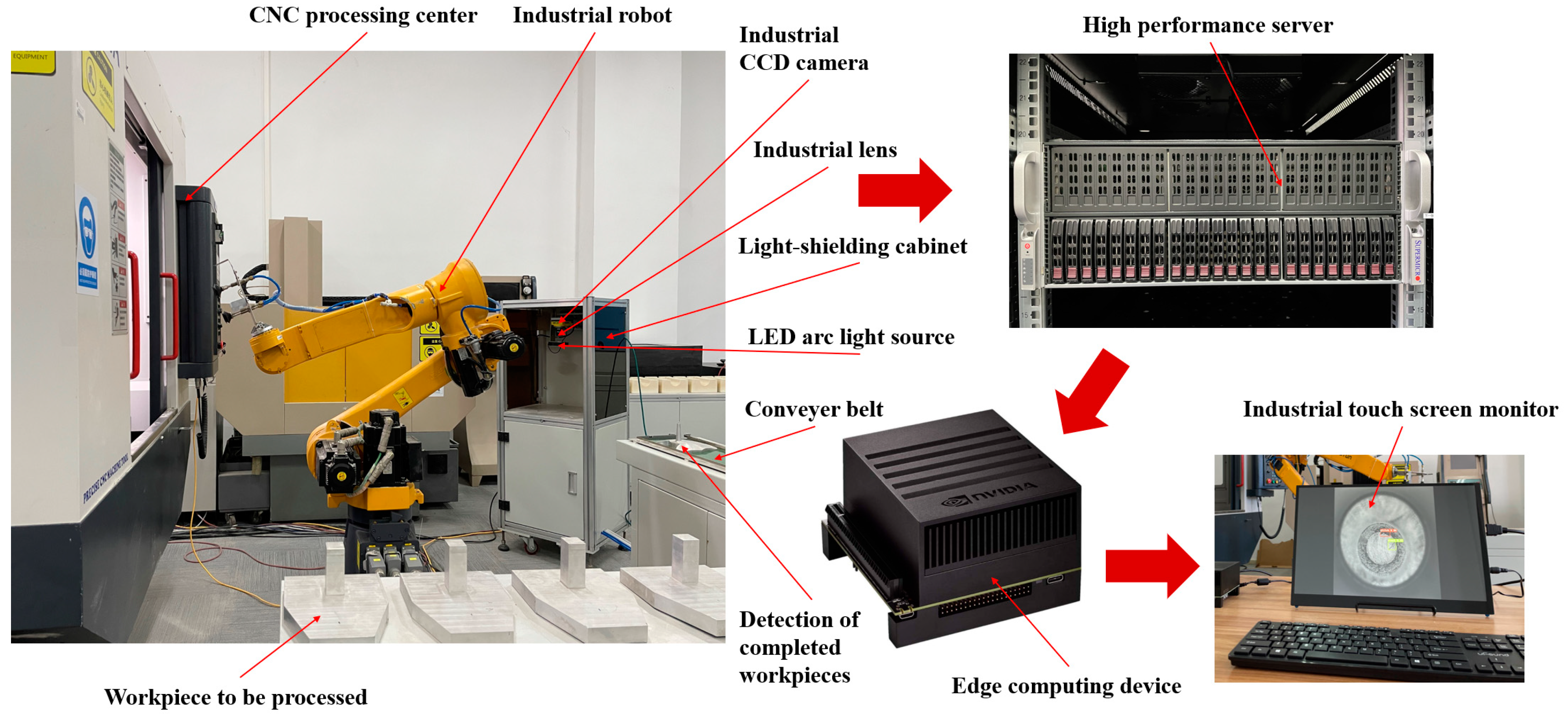
Figure 1. Image preprocessing flowchart.
Electronics 13 00253 g001
Figure 2. Data sample example image using the mosaic data augmentation method.
Electronics 13 00253 g002
Figure 3. The specific process of determining the initial estimation of anchor boxes using the K-means++ clustering algorithm.
Electronics 13 00253 g003
Figure 4. Technical route of the proposed method.
Electronics 13 00253 g004
Figure 5. Overall structure diagram of the product-surface-quality online inspection model.
Electronics 13 00253 g005
Figure 6. SPP’s structure diagram.
Electronics 13 00253 g006
Figure 7. FPN + PAN structure diagram.
Electronics 13 00253 g007
Figure 8. Channel pruning process diagram.
Electronics 13 00253 g008
Figure 9. Pruning process flowchart.
Electronics 13 00253 g009
Figure 10. Knowledge distillation structure diagram.
Electronics 13 00253 g010
Figure 11. Physical image of workpiece-surface-quality online inspection device.
Electronics 13 00253 g011
Figure 12. The training process of surface-quality online detection model (YOLOV4).
Electronics 13 00253 g012
Figure 13. The training process of the YOLOV4-tiny model.
Electronics 13 00253 g013
Figure 14. The specific distribution of Gamma coefficients of the BN layers before sparse training.
Electronics 13 00253 g014
Figure 15. The numerical values of the Gamma coefficients of the BN layers before sparse training.
Electronics 13 00253 g015
Figure 16. The specific distribution of Gamma coefficients of the BN layers during the sparse training process.
Electronics 13 00253 g016
Figure 17. The change in Gamma coefficients of the BN layers during the sparse training process.
Electronics 13 00253 g017
Figure 18. The specific distribution of Gamma coefficients of the BN layers after sparse training.
Electronics 13 00253 g018
Figure 19. The numerical values of the Gamma coefficients of the BN layers after sparse training.
Electronics 13 00253 g019
Figure 20. Schematic representation of channel changes before and after pruning for each layer.
Electronics 13 00253 g020
Figure 21. The training process of the model without using knowledge distillation.
Electronics 13 00253 g021
Figure 22. The training process of the model using knowledge distillation method.
Electronics 13 00253 g022
Figure 23. The detection effect of online inspection model for product surface quality before and after improvement, (ad): the inspection results of the surface quality online detection mode; (eh): the inspection results of the compression-based surface-quality online detection model.
Electronics 13 00253 g023
Figure 24. Performance comparison chart of lightweight models.
Electronics 13 00253 g024
Table 1. Hardware selection table for workpiece-surface-quality online inspection device.
Equipment NameHardware ModelParameter
Industrial robotESTUN ER6-K6B-P-DAC380 V/3.4 KVA, maximum load 6 kg, Arm span 1600 mm, repeatable positioning accuracy ± 0.08 mm
Industrial CCD cameraCOGNEX 821-0037-1R24VDC ± 10%/500 mA, 1/1.8 UI inch CCD,
1600 × 1200
resolution (pixels)
Industrial lensCOMPUTAR M5018-MP250 mm focal length, F1.8 aperture, 2/3″ target surface size
LED arc light sourceAFT, RL12068WRing, PWM dimming
Light-shielding cabinetHomemadeShade: 42 cm × 55 cm,
cabinet: 50 cm × 50 cm × 122 cm
Table 2. Model training parameter table.
ParameterYOLOV4YOLOV4-Tiny
Number of batch training samples6464
Number of sample subsets88
Image width416416
Image height416416
Number of channels33
Momentum0.9490.949
Weight decay regularization coefficient0.00050.0005
Random rotation angle00
Randomly adjusted saturation1.51.5
Randomly adjusted exposure1.51.5
Randomly adjusted hues0.10.1
Learning rate0.00010.0001
Number of traversals150150
Table 3. Depth model performance statistics table.
Network ModelSSD-Inception V2SSD-Inception V3YOLOV3YOLOV4-TinyQuality Detection Model
Number of Epochs100100100150150
IoU0.500.500.500.500.50
mAP (%)70.5976.6592.5492.7497.50
Model size (MB)52.699423623.1244
FPS (f/s)35.530.330.256.632.8
Table 4. Model compression parameter table.
StageParametersNumerical Value
Sparse trainingBatch sample quantity8
Learning rate0.003
Sparsity rate0.001
Number of traversals2000
PruningChannel pruning ratio0.90
Number of layers pruning2
Fine-tuned pruned modelNumber of traversals100
Batch sample quantity8
Table 5. Test results after model compression.
ParametersOriginal ModelChannel PruningLayer Pruning
Total parameters63,953,8411,107,9041,080,754
Average accuracy mean (%)97.5095.1495.14
Model size (M)2444.304.19
Inference time (s)0.03050.01530.0147
Table 6. Lightweight model performance statistics.
ParametersMobileNetV1-SSDMobileNetV2-SSDYOLOV3-TinyYOLOV4-TinyYOLOV5SYOLOV8SPruning Model
AP(Dent)34.7778.3381.3793.6597.3798.8598.82
AP(Crack)61.6362.7982.2395.2497.4598.6398.35
AP(Glitch)5066.5975.6785.9492.8694.1593.26
AP(Fracture)73.574.6491.6596.1396.8498.9799.21
mAP54.9870.5982.7392.7496.1397.6597.41
Model size (MB)18.552.634.723.114.121.54.19
FPS (2080Ti)64.653.755.456.666.162.368.0
FPS (AGX Xavier)42.329.630.633.844.538.447.8
Disclaimer/Publisher’s Note: The statements, opinions and data contained in all publications are solely those of the individual author(s) and contributor(s) and not of MDPI and/or the editor(s). MDPI and/or the editor(s) disclaim responsibility for any injury to people or property resulting from any ideas, methods, instructions or products referred to in the content.

