An Efficient Adaptive Noise Removal Filter on Range Images for LiDAR Point Clouds

Abstract

Light Detection and Ranging (LiDAR) is a critical sensor for autonomous vehicle systems, providing high-resolution distance measurements in real-time. However, adverse weather conditions such as snow, rain, fog, and sun glare can affect LiDAR performance, requiring data preprocessing. This paper proposes a novel approach, the Adaptive Outlier Removal filter on range Image (AORI), which combines a projection image from LiDAR point clouds with an adaptive outlier removal filter to remove snow particles. Our research aims to analyze the characteristics of LiDAR and propose an image-based approach derived from LiDAR data that addresses the limitations of previous studies, particularly in improving the efficiency of nearest neighbor point search. Our proposed method achieves outstanding performance in both accuracy (>96%) and processing speed (0.26 s per frame) for autonomous driving systems under harsh weather from raw LiDAR point clouds in the Winter Adverse Driving dataset (WADS). Notably, AORI outperforms state-of-the-art filters by achieving a 6.6% higher F1 score and 0.7% higher accuracy. Although our method has a lower recall than state-of-the-art methods, it achieves a good balance between retaining object points and filter noise points from LiDAR, indicating its promise for snow removal in adverse weather conditions.

1. Introduction

The development of autonomous vehicle technology has recently attracted considerable attention and investment. A major challenge facing these vehicles is the ability to sense and maneuver through their environment without human intervention [1]. To overcome this challenge, autonomous vehicles use a combination of different sensors, such as cameras, LiDAR (Light Detection and Ranging), radar, and GPS, together with advanced algorithms and machine learning methods to make informed decisions and successfully navigate their environment [2,3,4]. Among these sensors, LiDAR is considered a critical component in enabling autonomous vehicles to effectively sense and understand their environment. In most cases, the fusion of these sensors provides impressive reliability and efficiency for autonomous vehicles [5,6,7,8,9,10,11].

LiDAR works by emitting a laser beam and measuring the time it takes for the beam to bounce back after hitting an object. By measuring the distance to objects in the vehicle’s environment, LiDAR can create a high-resolution 3D map of the vehicle’s surroundings [12]. This 3D map is used to detect and track objects such as other vehicles, pedestrians, and obstacles, and to help the vehicle navigate its environment. LiDAR can also be used to detect and measure the speed of other vehicles, which is important for determining safe distances and speeds for autonomous vehicles to travel. One of the main benefits of LiDAR is that it can provide accurate measurements in a wide range of lighting and weather conditions, making it a reliable sensor for use in autonomous vehicles [13,14,15,16,17]. However, the resolution of LiDAR has limitations, which can be overcome by integrating it with a camera [18]. This compatibility can help to address the weaknesses of LiDAR in object detection and recognition when using a deep learning approach [19,20,21,22].

While LiDAR is generally a reliable sensor for use in autonomous vehicles, certain weather conditions can affect its performance. One of the main problems with LiDAR in adverse weather conditions is visibility and noise. Heavy rain, snow, or fog can scatter the laser beams and reduce the sensor’s range or cause false readings [23,24,25,26,27]. In extreme cases, the sensor may not be able to detect any objects at all. In addition, glare from the sun or bright headlights can also affect the sensor’s ability to detect objects. As a result, current LiDAR sensors do not perform as well in adverse weather conditions as they do in clear weather, which is why autonomous vehicles are still in the development and testing phase and not fully ready for commercial use. To mitigate these issues, LiDAR data can be filtered to detect and remove unwanted clutter in adverse weather conditions. This process can improve its ability to detect objects in challenging conditions.

Recently, there has been a growing interest in processing LiDAR data. Figure 1 shows a LiDAR and camera fusion image from the Canadian Adverse Driving Conditions Dataset [28]. Figure 1a shows a typical LiDAR frame under light snow weather conditions. In ideal weather conditions, LiDAR can improve the visibility and reliability of automated vehicle systems. However, weather can have a negative impact on LiDAR performance [24,29,30,31]. Snow can limit the field of view of LiDAR and reduce its reliability, as shown in Figure 1b. This figure shows numerous snowflakes captured around the vehicle. These random snow particles can also interfere with the vehicle’s warning systems. The closer the snowflakes are to the vehicle, the denser they become, which could lead to serious accidents in autonomous vehicles. Therefore, removing snow particles and filtering noise from LiDAR data is critical to improving its quality and reliability.

Data processing from LiDAR sensors in adverse weather conditions can be challenging due to the increased noise and reduced signal-to-noise ratio caused by the weather [29,32]. The efficiency of traditional filters is significantly reduced on data from LiDAR. Therefore, advanced filtering techniques were proposed to remove noise from the LiDAR data [32,33,34]. Previous designs for filtering snow points from LiDAR data have shown impressive results. However, these filters also remove points that are part of actual objects, leading to the loss of valuable information from the LiDAR data.

Computer vision models have become increasingly proficient in recognizing patterns across various tasks, achieving prominent levels of efficiency and accuracy [35,36,37]. As such, their potential to address noise filtering problems is a natural extension of their capabilities. With the increasing use of sensors such as LiDAR in various applications, including autonomous vehicles, noise filtering has become a significant area of interest [38,39]. The ability to effectively filter out unwanted noise from sensor data is crucial in enhancing the accuracy of object detection and recognition. Recently, researchers have developed various noise filters to improve the performance of autonomous vehicles in extreme weather conditions [36,40,41,42]. Some filters use advanced machine learning techniques to detect and remove noise from sensor data [43,44], while others employ physical filters or signal processing techniques to achieve similar results [45,46,47]. These filters use a variety of techniques, such as denoising algorithms [33,48] and adaptive filtering [29,32] to remove unwanted noise from LiDAR data and enhance the accuracy of object detection and recognition. By improving the visibility of LiDAR sensors, these filters can help to increase the safety and reliability of autonomous vehicles, especially in challenging weather conditions where visibility is limited. As the development of autonomous vehicles continues to advance, the use of noise filters is likely to become increasingly important in ensuring the safety and efficiency of these vehicles. The researchers also achieved impressive results in their experiments and their approach may be useful for improving the performance of autonomous vehicles in extreme weather conditions.

However, these filters mainly focus on improving the quality of camera images [40,41,42,48,49,50], and their effectiveness on LiDAR data is not significant. On the other hand, image-based approaches are mainly used to train computer vision models [43,51,52], which are capable of recognizing patterns in data and filtering noise even in adverse weather conditions. However, deep learning models require large amounts of data for training and have high model complexity. To our knowledge, no research has focused on filtering noise from images generated from LiDAR data. Recognizing that the noise in these images inherits characteristics from the LiDAR data, we propose an adaptive filter to overcome the limitations of previous filters.

It is worth noting that even though the technology has been commercialized for years, the data processing from LiDAR in adverse weather conditions is still a challenging task. Therefore, autonomous vehicles are being thoroughly evaluated in various weather conditions to ensure a higher level of safety.

In this paper, we present a novel adaptive outlier removal on range image filter that aims to improve the accuracy and processing time for noise detection and removal from LiDAR data. We also evaluate the performance of the filter using experiments on the Winter Adverse Driving dataset (WADS) [53]. The main contributions of this research are:

• A comprehensive analysis of the influence of traditional methods on LiDAR point clouds and the introduction of a range image approach has been shown to be effective.
• The proposed AORI filtering method for the range image, which demonstrates high performance in terms of processing time and accuracy.
• An experiment on the WADS dataset under extreme weather conditions and a comparison with other existing methods in terms of accuracy, F1 score and execution time.

2. Related Work

The process of filtering noise from a LiDAR point cloud involves the elimination or reduction of extraneous data points that are not representative of the actual environment. This step is crucial, as LiDAR sensors are prone to producing false readings, such as outliers, due to environmental conditions or inherent sensor noise. The ultimate objective is to attain a precise and unadulterated representation of the environment, which is essential for a range of applications including autonomous navigation, object detection and scene comprehension.

There are several commonly used traditional methods for filtering noise from LiDAR point clouds, including statistical outlier removal (SOR) and radial outlier removal (ROR) [54,55]. Both SOR and ROR are techniques that eliminate data points that are significantly different from the majority of the data. These methods help to reduce errors or noise in Li-DAR point clouds, thereby improving the quality of the data. Noise is classified based on the clustering of the data. Errors or noise often occur randomly. Therefore, their density is sparser than the object points. Traditional filters classify data according to this characteristic. The advantage of traditional methods is that they are fast. However, accuracy and reliability are not high.

Traditional filters are usually quite simple, while the data density of objects in LiDAR is different. Therefore, several adaptive filters have been proposed to solve this problem, such as dynamic statistical outlier removal (DSOR) [53] and dynamic radius outlier removal (DROR) [29]. DROR generates an adaptive search radius that can be changed depending on the distance between the object and the LiDAR. DSOR has a similar idea. The mean distance is varied by distance to account for the change for each point in the entire LiDAR data. The effectiveness of the filter is improved by accounting for the decrease in density of object point clouds with increasing distance from the LiDAR. This is achieved by defining the search radius as the product of a multiplier constant and the distance to the object. The results of DSOR and DROR show that the proposed method achieves more than 90% accuracy on the LiDAR point cloud without removing environmental features.

In another aspect, deep learning models offer an opportunity to address this challenge, utilizing techniques such as denoising algorithms, adaptive filtering, and temporal filtering to effectively remove noise from the data [56]. As these models continue to evolve, their potential to improve the accuracy and reliability of sensor data will undoubtedly play a significant role in advancing many fields, including autonomous vehicles, robotics, and healthcare. The researchers applied computer vision to noise classification from LiDAR. Data from LiDAR will be converted to an image format. These images will be fed into the training model to detect features to identify noise from the image. Wheathernet [43] and 4DenoiseNet [44] have been shown to be effective in improving data quality from LiDAR in this approach. In certain scenarios, deep learning methods may outperform traditional approaches. However, traditional supervised learning algorithms rely heavily on large, labeled datasets to train models, making them less effective when labeled data are limited. Unsupervised learning, on the other hand, allows for the exploration and discovery of hidden patterns and structures within the data without the need for explicit labeling [57]. This enables the model to generalize better and achieve higher accuracy even when limited labeled data are available.

The intensity approach has also received much attention in recent studies. Low-intensity outlier removal (LIOR) [45] pioneered the use of point intensities in LiDAR data sets in conjunction with traditional filtering for noise detection. High-intensity object points are removed. As a result, filter performance is significantly improved. However, the filtering performance still needs to be improved. Some combined adaptive filtering methods using intensity have been proposed to overcome these limitations, such as Dynamic Distance–Intensity Outlier Removal (DDIOR) [46] and Adaptive Group of Density Outlier Removal (AGDOR) [58]. The main advantage of these filters is that they can handle point clouds with different densities more effectively. In areas of high point density, the search radius is small, resulting in more aggressive outlier removal, while in areas of low point density, the search radius is larger, resulting in more lenient outlier removal. Dynamic Light–Intensity Outlier Removal (DIOR) [47] has an efficient FPGA approach that can improve both accuracy and performance.

However, the precision and recall of these filters have always been significantly different. Therefore, these filters always tradeoff between noise detection and noise removal targeting object points. Therefore, our proposed method is introduced to overcome their limitations. In this study, we do not use LiDAR point clouds directly, but generate depth images from them. The depth images are denoised based on the adaptive filtering method presented in the proposed filter section. This approach can improve more than 96% for accuracy and nearly 90% for the F1 score on the WADS dataset. The filter can retain the object points, which is a particularly important factor in an autonomous driving system. Furthermore, our proposed filter has been adopted to improve the execution time of the system.

3. The Proposed Filter

Adaptive noise filter on range image is a novel approach for classifying snow points from the LiDAR point cloud. As the fact is that the scan lines of LiDARs are not uniformly spaced in the vertical axe, our raw point clouds obtained from LiDAR will be converted to range image data. All the processes or filtering will be performed in the frame of the range images. This innovative approach is unique compared to previous filters. Anomalies from pixels in the image will be detected and eliminated by our proposed method. The general structure of the filter is depicted in Figure 2. There are two main parts in the proposed method: image conversion, and adaptive noise filter for range images from LiDAR. In this section, the details of each step will be introduced.

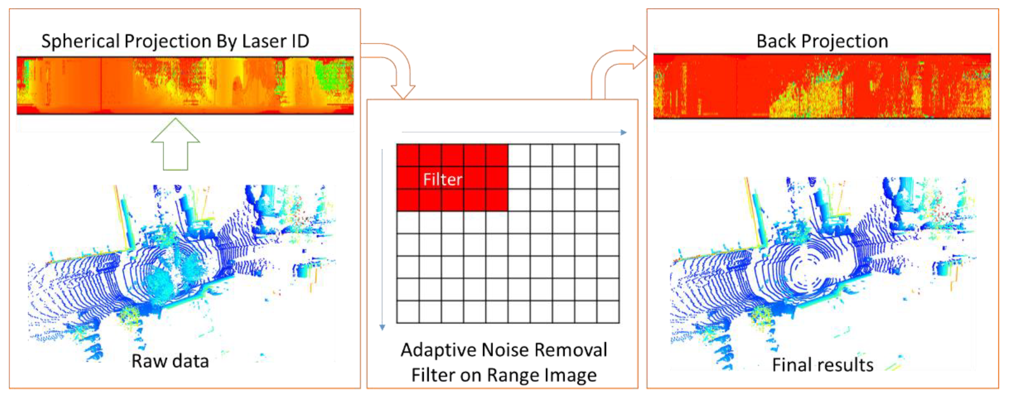
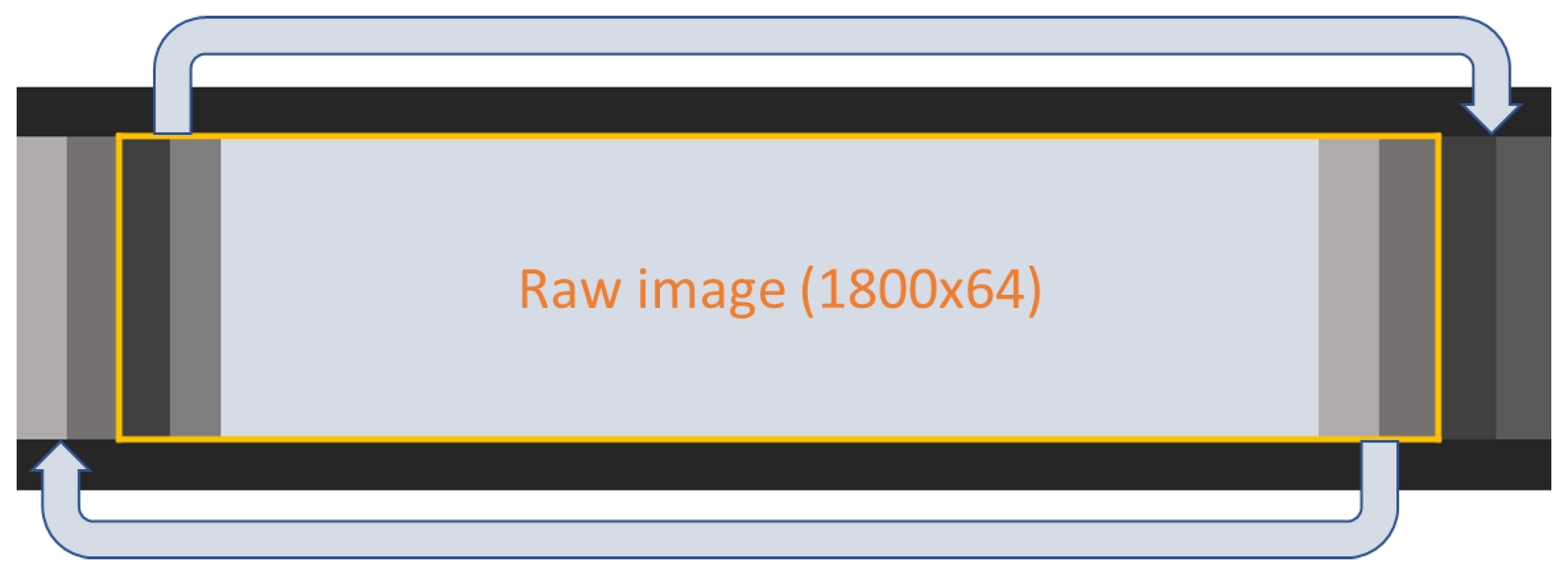
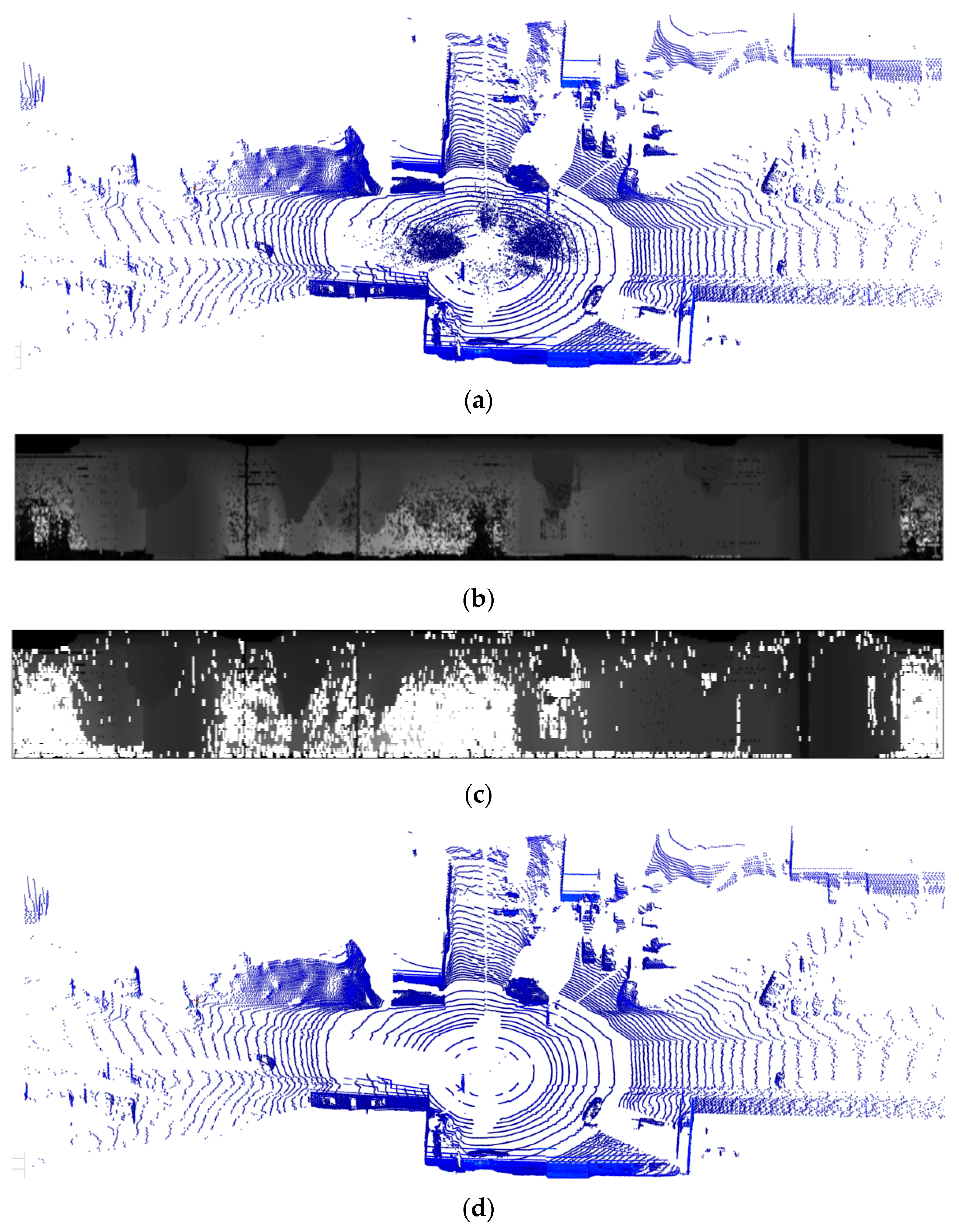
3.1. Generating the Range Image

The spacing between elevation angles from diverse types of LiDAR is not uniform. As a result, the distribution of data obtained from LiDAR is not uniform in density. The density of the central point differs significantly at the top and bottom of the vertical field of view, as shown in Figure 3. The uniformity of the horizontal resolution of a LiDAR system is well established, while the vertical resolution is a significant disparity. Therefore, traditional filters are challenged at the top and bottom lasers due to the large elevation angle. To solve this problem, our proposed approach focuses on 2D range images where the distribution of pixels is the same over the entire data. Furthermore, it is worth noting that the 2D image representation can also capture the local geometric properties of the LiDAR data. By exploiting this intrinsic property, it is possible to obtain the neighboring points of each LiDAR point without the need to construct a KD-tree.

Creating a range image from LiDAR data involves converting the 3D point cloud data into a 2D representation showing the distances between the LiDAR sensor and the objects in the scene. Each point in WADS contains four data fields including [X, Y, Z, and Intensity]. X, Y, and Z are Cartesian coordinates in 3D space. Normally, traditional filters use values from these coordinates to find relationships between points and distinguish them from noisy points. However, we found that the uneven distribution of elevation angles from the LiDAR significantly reduces the efficiency of the filters. Figure 3 shows the distribution of elevation angles from LiDAR Pandar64. In addition, the horizontal data points are much denser compared to the vertical distribution. Therefore, these issues affect the filtering of noise from the filter based on the raw data point clouds, where the previous filters suggested a density-based noise classification. The difference in resolution between the horizontal and vertical axes of LiDAR is significant, particularly for the upper and lower lasers. As a result, a larger search radius is required to identify neighboring points in adjacent lasers. However, this significantly reduces the ability of the filters to remove noise. To overcome this problem, we propose a novel approach using projected images derived from LiDAR point clouds. The point clouds are rescaled to pixels in a 2D image where the resolution between points is similar. On the other hand, the 2D image representation allows for the capture of the local geometry of the LiDAR data, allowing for the easy detection of neighboring points without the need to construct a KD-tree.

The spherical projection process was applied to convert LiDAR point clouds to 2D range images which was shown in Figure 4. The distance (r), vertical angle ($\theta$), and horizontal angle ($\phi$) of the points can be calculated as:

$$\left\{\begin{array}{c}r=\sqrt{x^2+y^2+z^2}\\ \phi =\arctan \frac{x}{y}\\ \theta =\arctan \frac{z}{r}\end{array}\right..$$

(1)

This step involves transforming the three-dimensional point cloud data into a two-dimensional representation through a process called scan conversion. The process involves mapping each 3D point in the point cloud to a specific pixel in the 2D image.

Subsequently, the 3D points in the point cloud are projected onto the 2D image plane through either a perspective or orthographic projection method. The column and row index of the range image are represented by u and v, respectively.

To align with the vehicle’s heading direction, the center column of the range image should be calculated using the formula for u, which can be expressed as:

$$u=\left[\frac{1}{2}\left(1+\frac{\phi }{\pi }\right)·w\right],$$

(2)

where $w$ represents the width from the Range Image. $w$ was determined based on the horizontal resolution of LiDAR ($r_h$) using the following formula:

$$w=\frac{{360}^{°}}{r_h}$$

(3)

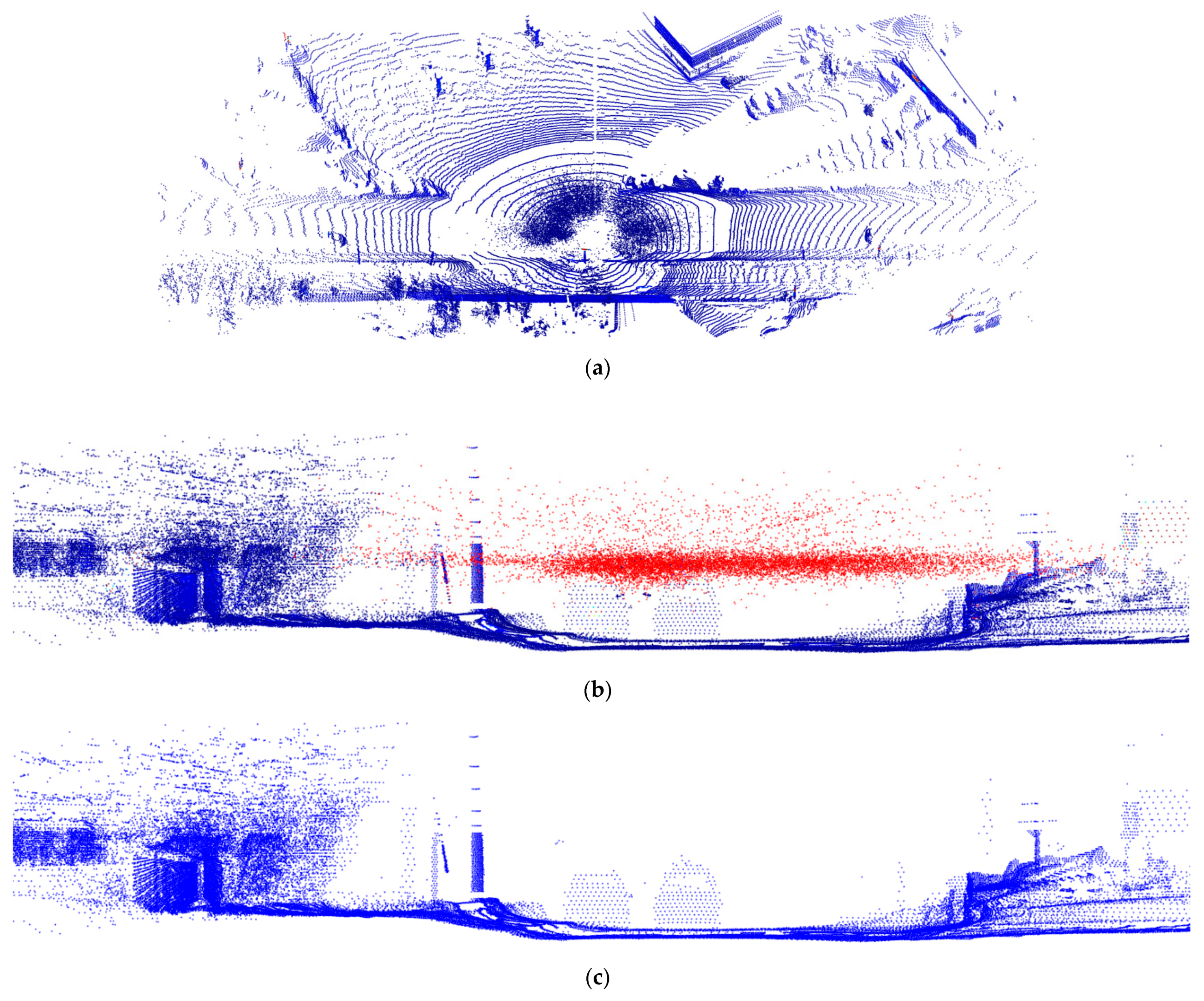
3.2. Adaptive Noise Removal Filter on Range Image

In this step, our goal was to detect snow particles based on range image data. We observed that snow particles appeared randomly in the range image and were characterized by a lower density compared to objects. The unique characteristics of snow particles in contrast to objects, such as their irregular distribution and lack of clustering, allowed our proposed method to exploit the inherent properties of the LiDAR dataset, where the distance between points tends to increase with distance. Therefore, we introduced an adaptive filter that can effectively detect and remove snow particles in the range image.

The idea for this filter is based on detecting neighboring pixels that satisfy the distance condition. The distance of neighboring pixels must be less than the search radius (SR). Hence, we filtered the correlation for this case. A label matrix was generated during cross-correlation filtering ${(L}_{\left(a,b\right)})$. To accommodate the unique nature of LiDAR data, the adaptive filter described in this work incorporated a kernel of size 5 × 3 (K) to determine the label of each pixel in the sliding window, and padding was added to maintain the size of the label matrix during cross-correlation filtering. Figure 5 illustrates the padding process for 2D range images from our proposed method. However, because the data between the first and last columns of the image are sequential, the padded image matrix ($R_{a,b}$) was adjusted according to the following formula:

$$\left\{\begin{array}{c}Rp\left[1:a-1,2:b-2\right]=R\left[u,v\right]\\ Rp\left[1:a-1,0:1\right]=R\left[:,v-2:v\right]\\ Rp\left[1:a-1,b-1:b\right]=R\left[:,0:2\right]\end{array}\right..$$

(4)

The set $F_{a,b}\left(F_{a,b}\in Rp\right)$, which was called the distance to the center from the nearest neighbor group, was recognized by the following formula:

$$F_{a,b}=abs\left(R_{a-2:a+2,b-1:b+1}-R_{a,b}\right)$$

(5)

where $a,b$ is column and row coordinates from the $R_{a,b}$.

Neighboring points (P) were determined based on the search radius (SR) and neighboring pixels. The difference between neighboring pixels less than SR was defined as a neighbor point:

$$P_{a,b}=F_{a,b}(F_{a,b}<{SR}_{a,b}).$$

(6)

However, to accommodate the distance-based variable densities of the LiDAR data, the proposed search radius is an equation according to the following formula:

$${SR}_{a,b}=\alpha \times \theta \times R_{a,b},$$

(7)

where $\alpha$ is the multiplier factor for the filter, and $\theta$ is the angular resolution (azimuth) of LiDAR. $\theta$ is different depending on the LiDAR model.

Then, the total points $N_{\left(a,b\right)}$ were a count from the set $F_{\left(a,b\right)}$. Core points and outlier were identified based on the numbers of neighbor $(NoN$) and $N_{F_i}$:

$$L_{\left(a,b\right)}=\left\{\begin{array}{c}1 if NoN\le N_{\left(a,b\right)} (core point)\\ 0 if NoN>N_{\left(a,b\right)} \left(outlier point\right)\end{array},\right.$$

(8)

Our approach to noise filtering based on the range image generated by LiDAR represents a novel methodology. The search radius and a minimum number of neighboring points were determined by previous studies, and the performance of our filter was significantly improved by grouping neighboring points and labelling them together with the core points. This approach optimizes the computation time of the filter. In addition, we incorporated an input checker in the second stage, which eliminated the need to check all input points by grouping neighboring objects with the core point. The complete flow of our filter is shown in Algorithm 1.

Algorithm 1 Pseudocode of our proposed filter

Input: $R\left[u,v\right]$ % Projection range image by laser ID from $P=\left\{p_1,p_2,\dots ,p_n\right\}$    Output: Snow Points, Object Points    Def filterRangeImage:      $Rp$ = paddingRangeImage(R)      $\mathrm{L}\leftarrow \mathit{z}\mathit{e}\mathit{r}\mathit{o}\mathit{s}\left(R_{rows}\times R_{cols}\right)$      for $a=1:R_{rows}$ do:        for $b=1:R_{cols}$ do:             if $L_{\left(a,b\right)}=0$:               $\mathrm{S}\mathrm{R}=\alpha \times \theta \times R_{a,b}$               $F_{a,b}=abs\left({Rp}_{a-2:a+2,b-1:b+1}-R_{a,b}\right)$                        $P_{a,b}=F_{a,b}(F_{a,b}<{SR}_{a,b}).$                 count the number of $P_{a,b}$ ($N_P$)              if $NoN$ $\le N_{\mathrm{P}}$ then                   $P_{a,b}$ ← object points (inlier)               else                   $R_{a,b}$ ← noise point (outlier)               end if             end if           end for         end for.    Def paddingRangeImage(R):      $Rp=zeros\left(h+2,w+4\right)Rp=zeros\left(h+2,w+4\right)$      $Rp\left[1:h+1,2:w+2\right]=R$      $Rp\left[1:h+1,0:1\right]=R\left[:,w-2:w\right]$      $Rp\left[1:h+1,w+3:w+4\right]=R\left[:,0:2\right]$       return $Rp$.

4. Experimental Results

To evaluate the effectiveness of our proposed method under challenging conditions, we conducted experiments on the Winter Adverse Driving dataset (WADS) and compared our results with those obtained using existing methods. In this section, we provide a brief overview of the dataset and outline the parameter settings for the filtering and evaluation metrics. We then evaluate the performance of our proposed filter in terms of accuracy and compare it with other methods, including ROR, SOR, LIOR, DROR, DSOR, DDIOR, and AGDOR.

4.1. Experimental Dataset

The Winter Adverse Driving dataset is the first publicly available dataset labeled with snow particles on each point cloud. The dataset consists of 19 scenes, each containing approximately 100 frames with more than 200,000 points per frame, and each point is labeled with one of 22 classes. In our experiment, we were only interested in the subclasses that are snow particles and non-snow particles. The dataset is diverse in terms of weather conditions, ranging from light to extreme snowfall. Hence, it was suitable to apply in experiments to prove our filter efficiency. Previous datasets used in similar research were limited and heterogeneous, making this dataset ideal for evaluating the generality and effectiveness of our proposed model.

4.2. Experimental Settings

The filters we chose for the comparison in this experiment included two main types: the traditional filter (ROR and SOR) and the state-of-the-art filters (LIOR, DROR, DSOR, DDIOR, and AGDOR). Compared filters were executed in Python language on the same workstation for reliability. The workstation with Intel^® Xeon^® Silver 4114 CPU @2.20 GHz, GRID Virtual GPU V100D-8Q, and 32GB RAM memory was utilized in our experiment.

The experimental results of our proposed method were affected by the multiplier value for the search radius (α) and the minimum number of neighbors (NoN). In this experiment, α and NoN were chosen based on the results of previous studies. To prove the reliability of our proposed method, we kept the same parameters as the previous filters. The parameters of the filters in the experiment are shown in

Table 1. Filter Parameters.

Method	Parameters	Value
ROR	NoN	5
	Search radius	0.1 m
SOR	NoN	5
	Standard deviation	0.1
DROR	Search radius	5
	Radius multiplier	3
	Azimuth angle	0.1°
DSOR	NoN	5
	Multiplicative	0.05
	Global threshold constant	0.1
LIOR	Search radius	0.1 m
	NoN	5
	Snow detection range	71.235 m
	Intensity threshold	9
DDIOR	NoN	5
AGDOR	NoN	5
	Multiplier factor	0.001
	Intensity threshold	9

.

4.3. Evaluation Metrics

To assess the effectiveness of the filter in harsh weather conditions, we used a 2 × 2 confusion matrix to classify four noise filtering outcomes: True Positive (TP), True Negative (TN), False Positive (FP), and False Negative (FN). A TP represents an instance where the filter correctly identifies the snow class, while a TN represents an instance where the filter correctly identifies the object class. Conversely, an FP represents an instance where the filter incorrectly identifies the snow class, and an FN represents an instance where the filter incorrectly identifies the object class. A filter is defined as good if it can filter out most of the noise while retaining most of the objects. Filters often choose a compromise between these two parameters in most cases. Therefore, to evaluate the influence of the above two values, the F1 score was used as a criterion to evaluate the effectiveness of the filter. F1 scores were developed that rely on both precision and recall. On the other hand, the execution time is also of interest in the comparison. The five metrics used in the evaluation were execution time, accuracy (“Acc”), precision (“Pre”), recall (“Re”), and F1 score (F1). While accuracy is a commonly used metric in classification problems, it can be misleading in WADS (unbalanced) datasets where the number of object points is significantly larger than the number of snow noise points. In such cases, a model that simply predicts the object class for all samples may achieve high accuracy but fail to detect the snow class. The F1 score takes into account both precision and recall and provides a more accurate assessment of a model’s performance in such scenarios. A higher F1 score indicates a better balance between precision and recall, which is important in many practical applications.

4.4. Implementation Results

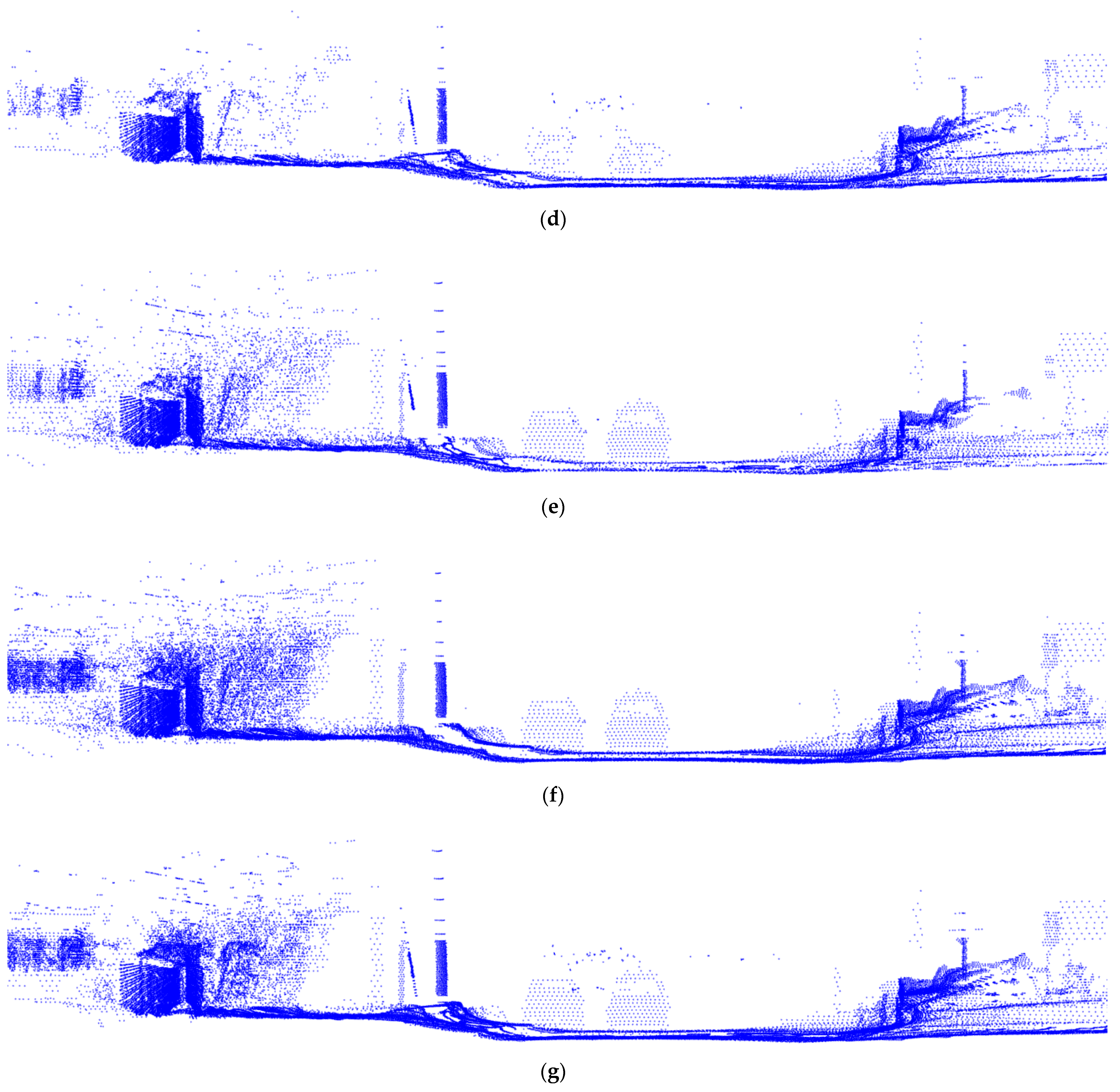
Determining the optimum parameter values for the filter is crucial to improving its ability to detect and remove noise points. The choice of multiplier value affects the search radius, and a large search radius may inadvertently include snow particles. A smaller search radius will result in more aggressive outlier removal, while a larger search radius will improve the efficiency of the retaining feature points. In our experiments, we found that a multiplier of 0.01 and a “NoN” (minimum number of neighbors) of five gave the best filter performance compared to another study. It is also important to consider the execution time of the filter. The processing time increases as the search radius decreases or the minimum number of neighbors increases. However, as the search radius increases, the number of neighbors also increases, making it easier to determine their labels without the need for an algorithm. Our experiments were designed to evaluate the effectiveness of the filter in harsh environments.

The performance of our proposed filter on the Winter Adverse Driving dataset is illustrated in Figure 6. The raw LiDAR point clouds from the dataset are shown in Figure 6a, which contains numerous snow particles collected by LiDAR. Figure 6b shows the projection area image from the raw LiDAR point clouds, while Figure 6c shows the area image after applying our proposed filter, which removes the detected snow points, resulting in the appearance of many white points. The final image shows the result after projection from the filtered range image. We also present the results of our algorithm and four comparison methods for this dataset. The clear image is shown in Figure 6d after removing the snow points from the ground truth.

Snow particles in Figure 7a have a high density, which is a challenge for traditional noise filters. Due to the sensitivity of point cloud density to distance, traditional density-based filters are ineffective at detecting snowflakes. Previous studies of traditional filters without density adjustments resulted in missing long-range information. The object points appear dense, and it is difficult to observe the difference between the methods. Therefore, we simulated LiDAR with a vehicle view, which has not been simulated in previous studies. Figure 6b shows a LiDAR raw data frame from the vehicle perspective. Object points are marked in blue, while noise points caused by snow particles are marked in red. On the other hand, DROR and LIOR are more efficient at filtering noise, but still lose important data points. Most of the important features of the data are retained. However, there is a trade-off between the ability to filter noise and the retention of important data points. The higher the efficiency of snow detection, the more important data points are lost. The results of DSOR are simulated in Figure 7g. The experimental results of DSOR show an impressive performance in object point retention. Unfortunately, the snow noise is not completely removed. Our proposed filter overcomes this limitation and achieves high precision and recall, as shown in Figure 6c. The filter effectively removes the dense density of snow particles while retaining most of the critical object information. In heavy snow conditions, our filter cleans the input LiDAR data without losing essential features.

4.5. Evaluation

In this section, we will evaluate the filter’s performance by comparing its processing time and accuracy with those of the SOR, ROR, DROR, DDIOR, AGDOR, and LIOR filters. The results presented in

Table 2. Comparison of the proposed filter.

Methods	Acc (%)	Pre (%)	Re (%)	F1 (%)	Execution Time (s)
SOR	79.57	32.73	21.96	26.98	0.21
ROR	62.5	67.79	18.19	28.68	0.25
LIOR [45]	90.35	66.17	55.56	60.4	0.07
DROR [29]	96.17	71.91	91.89	80.68	10.99
DSOR [53]	95.77	65.07	95.6	77.43	0.2
DDIOR [46]	96.26	69.87	95.23	80.6	1.3
AGDOR [58]	96.15	96.19	80.59	83.3	0.51
Our filter	96.96	87.9	89.92	89.9	0.26

provide an overview of the filter’s efficiency.

The performance of the proposed filter was evaluated using several metrics such as accuracy, precision, recall, and F1 score. While conventional filters have a simple structure and faster processing time, they failed to detect object points. On the other hand, the LIOR filter showed a significant increase in recall, while intensity-based filters were more efficient in reducing false positive rates. However, the second-step radius outlier removal was not effective in classifying low-intensity data points. The DROR, DSOR, and DDIOR filters showed higher precision and recall than LIOR, but had a high rate of false negatives, which resulted in the loss of valuable information from the LiDAR, affecting object recognition and driver safety.

The F1 score provides a balanced measure of both precision and recall. Precision measures the proportion of snow points among all the predicted snows, while recall measures the proportion of snow points among all the actual snows in the dataset. High precision means that the accuracy of the points found is high. High recall means a high True Positive Rate, which means that the rate of missing actual snow points is low. A high F1 score indicates that the model is effective in detecting both types of object and noise points.

Our proposed method shows a significant improvement in Table 2, as indicated by the increase in accuracy of 6.61%, 0.79%, 1.19%, 0.7% and 0.81% on LIOR, DROR, DSOR, DDIOR, and AGDOR, respectively. In particular, the precision of our method increased by 21.73%, 15.99%, 22.83%, and 18.03% on LIOR, DROR, DSOR, and DDIOR, respectively, although it was lower than that of AGDOR, indicating that our filter retains feature points. Although our accuracy results were impressive, our recall results were lower than previous studies, specifically 1.97%, 5.68% and, 5.31% for DROR, DSOR, and DDIOR, respectively. We attribute this to our attempt to reduce the search radius, which resulted in the removal of important feature points. This finding highlights the trade-off between removing noise and retaining important points and may guide future research in this area to improve recall. Although these results may be disappointing, they provide valuable insights into the limitations of our approach and the weaknesses of previous filters, which often resulted in a significant difference between precision and recall. While recall is important for identifying all relevant objects in the data, precision is also critical in ensuring that the identified objects are accurately classified. In this case, our method may be sacrificing some recall for better precision, resulting in a higher F1 score. We recognized the importance of these two factors and optimized our filter accordingly. As a result, the F1 score increased significantly by 29.5%, 9.22%, 12.47%, 9.3% and 6.6% for LIOR, DROR, DSOR, DDIOR, and AGDOR, respectively. The range image approach effectively preserves object points at different elevation angles, although it has limitations in detecting snow points close to objects. The conversion of input data into image data is a limitation of our method, resulting in increased filter execution time. Nevertheless, our proposed method achieves a significantly higher number of results than the compared filters.

The processing time is presented in Table 2 along with the other experimental results. The use of 2D images allows the local geometry of the LiDAR data to be captured, which makes it easy to capture neighboring points without the need to construct a KD-tree. Therefore, our proposed method can improve the processing time compared to previous filters. The comparative methods use the KD-tree algorithm to find the nearest neighbor, which has a time complexity of O (D × N × logN), where D is the dimensionality of the data and N is the number of points obtained from LiDAR. On the other hand, the proposed image-based approach directly obtains neighborhood points, which significantly reduces the computational complexity. However, the number of pixels in the range image is generally higher than the total number of points obtained from LiDAR, due to undefined pixels where the LiDAR signal does not receive a response, which increases the execution time. Fortunately, this increase is negligible, resulting in a significant improvement in the overall execution time. As a result, our proposed method shows significant improvements in processing time compared to state-of-the-art methods. Specifically, the adaptive range image approach is five times faster than DDIOR and twice as fast as AGDOR. Furthermore, the point grouping method successfully reduces the execution time. However, our proposed filter is still two times slower than LIOR and comparable to DSOR and traditional filters.

Since the performance evaluation of the filter is not a simple task, we may propose a figure of merit (FOM) to estimate the whole performance of our filter. It can be quantitatively defined as the error of filter and FPS which represent the frames per second (1/Execution time). Let’s define the performance factor as:

$$\mathrm{FOM}=\frac{\mathrm{FPS}}{100-\sqrt[4]{Acc\times Pre\times Re\times F1}},$$

(9)

Under this definition, the FOM of our filter gets higher performance than the FOMs for the other methods. With this rule, it can be found that the performance of our filter would be better than the other traditional methods. That is, our filter performance does an excellent job in keeping high accuracy at a low computing power.

5. Discussion

Based on our experimental results, the adaptive range image approach effectively solves two major problems: the ability to detect snow in extreme weather conditions and the improved processing time for high-resolution data frames. Our proposed method demonstrates exceptional performance, as indicated by its excellent F1 score coefficient, which confirms its superior ability to retain object points while detecting and removing noise points. This translates into increased reliability of LiDAR sensors in vehicles. Furthermore, our approach exhibits the highest accuracy among the methods compared, making it highly suitable for use in extreme weather conditions. Our results are validated on the WADS dataset, which consists of approximately 1800 frames distributed across 18 sequences.

However, the volume of data generated by LiDAR sensors presents a significant challenge in terms of processing time. Our method provides an effective solution, although it is still slower than traditional methods and unsuitable for real-time systems. Future improvements could include data dimensionality reduction methods to overcome this limitation. Another limitation is the pre-processing step required to convert LiDAR point clouds into images, although we could potentially bypass this step by directly using the laser ID from the LiDAR.

6. Conclusions

The results of our proposed method demonstrate its exceptional performance in operating effectively in extreme environments, a challenging task in recent LiDAR sensor studies. Experiments conducted on the WADS dataset confirm that the proposed algorithm effectively reduces unwanted snow points during data acquisition. The range image approach, in particular the projection range image and the density filter, proved to be useful and effective. After applying the proposed filter, the F1 score and accuracy were the best under all weather conditions, achieving a trade-off between filter performance and execution time. With an F1 score of around 90%, our proposed method is satisfactory, especially for the vehicle’s driver assistance system. We believe that an accuracy of at least 95% is ideal for a combination model. The proposed filter can help the LiDAR work more efficiently and improve its efficiency in extreme environments. This represents a new direction for filtering noise from LiDAR point clouds and a new pre-processing for the computer vision approach.

References

1. Martínez-Díaz, M.; Soriguera, F. Autonomous Vehicles: Theoretical and Practical Challenges. Transp. Res. Procedia 2018, 33, 275–282. [Google Scholar] [CrossRef]
2. Yeong, D.J.; Velasco-hernandez, G.; Barry, J.; Walsh, J. Sensor and Sensor Fusion Technology in Autonomous Vehicles: A Review. Sensors 2021, 21, 2140. [Google Scholar] [CrossRef] [PubMed]
3. Hu, J.W.; Zheng, B.Y.; Wang, C.; Zhao, C.H.; Hou, X.L.; Pan, Q.; Xu, Z. A Survey on Multi-Sensor Fusion Based Obstacle Detection for Intelligent Ground Vehicles in off-Road Environments. Front. Inf. Technol. Electron. Eng. 2020, 21, 675–692. [Google Scholar] [CrossRef]
4. Fayyad, J.; Jaradat, M.A.; Gruyer, D.; Najjaran, H. Deep Learning Sensor Fusion for Autonomous Vehicle Perception and Localization: A Review. Sensors 2020, 20, 4220. [Google Scholar] [CrossRef] [PubMed]
5. Xu, D.; Anguelov, D.; Jain, A. PointFusion: Deep Sensor Fusion for 3D Bounding Box Estimation. In Proceedings of the IEEE Computer Society Conference on Computer Vision and Pattern Recognition, Honolulu, HI, USA, 21–26 July 2017; pp. 244–253. [Google Scholar]
6. Shahian Jahromi, B.; Tulabandhula, T.; Cetin, S. Real-Time Hybrid Multi-Sensor Fusion Framework for Perception in Autonomous Vehicles. Sensors 2019, 19, 4357. [Google Scholar] [CrossRef] [PubMed]
7. Norbye, H.G. Camera-Lidar Sensor Fusion in Real Time for Autonomous Surface Vehicles. Norwegian University of Science and Technology, Norway. 2019. Available online: https://folk.ntnu.no/edmundfo/msc2019-2020/norbye-lidar-camera-reduced.pdf/ (accessed on 12 March 2023).
8. Yang, J.; Liu, S.; Su, H.; Tian, Y. Driving Assistance System Based on Data Fusion of Multisource Sensors for Autonomous Unmanned Ground Vehicles. Comput. Netw. 2021, 192, 108053. [Google Scholar] [CrossRef]
9. Kang, D.; Kum, D. Camera and Radar Sensor Fusion for Robust Vehicle Localization via Vehicle Part Localization. IEEE Access 2020, 8, 75223–75236. [Google Scholar] [CrossRef]
10. Wei, P.; Cagle, L.; Reza, T.; Ball, J.; Gafford, J. LiDAR and Camera Detection Fusion in a Real-Time Industrial Multi-Sensor Collision Avoidance System. Electronics 2018, 7, 84. [Google Scholar] [CrossRef]
11. De Silva, V.; Roche, J.; Kondoz, A. Robust Fusion of LiDAR and Wide-Angle Camera Data for Autonomous Mobile Robots. Sensors 2018, 18, 2730. [Google Scholar] [CrossRef]
12. Li, Y.; Ibanez-Guzman, J. Lidar for Autonomous Driving: The Principles, Challenges, and Trends for Automotive Lidar and Perception Systems. IEEE Signal Process. Mag. 2020, 37, 50–61. [Google Scholar] [CrossRef]
13. Wolcott, R.W.; Eustice, R.M. Visual Localization within LIDAR Maps for Automated Urban Driving. In Proceedings of the 2014 IEEE/RSJ International Conference on Intelligent Robots and Systems, Chicago, IL, USA, 14–18 September 2014; pp. 176–183. [Google Scholar]
14. Murcia, H.F.; Monroy, M.F.; Mora, L.F. 3D Scene Reconstruction Based on a 2D Moving LiDAR. In Applied Informatics, Proceedings of the First International Conference, ICAI 2018, Bogotá, Colombia, 1–3 November 2018; Communications in Computer and Information Science; Springer: Cham, Switzerland, 2018; Volume 942. [Google Scholar]
15. Li, H.; Liping, D.; Huang, X.; Li, D. Laser Intensity Used in Classification of Lidar Point Cloud Data. In Proceedings of the International Geoscience and Remote Sensing Symposium (IGARSS), Boston, MA, USA, 6–11 July 2008; Volume 2. [Google Scholar]
16. Akai, N.; Morales, L.Y.; Yamaguchi, T.; Takeuchi, E.; Yoshihara, Y.; Okuda, H.; Suzuki, T.; Ninomiya, Y. Autonomous Driving Based on Accurate Localization Using Multilayer LiDAR and Dead Reckoning. In Proceedings of the IEEE Conference on Intelligent Transportation Systems, Yokohama, Japan, 16–19 October 2017; pp. 1–6. [Google Scholar]
17. Jang, C.H.; Kim, C.S.; Jo, K.C.; Sunwoo, M. Design Factor Optimization of 3D Flash Lidar Sensor Based on Geometrical Model for Automated Vehicle and Advanced Driver Assistance System Applications. Int. J. Automot. Technol. 2017, 18, 147–156. [Google Scholar] [CrossRef]
18. Ahmed, S.; Huda, M.N.; Rajbhandari, S.; Saha, C.; Elshaw, M.; Kanarachos, S. Pedestrian and Cyclist Detection and Intent Estimation for Autonomous Vehicles: A Survey. Appl. Sci. 2019, 9, 2335. [Google Scholar] [CrossRef]
19. Wen, L.H.; Jo, K.H. Fast and Accurate 3D Object Detection for Lidar-Camera-Based Autonomous Vehicles Using One Shared Voxel-Based Backbone. IEEE Access 2021, 9, 1. [Google Scholar] [CrossRef]
20. Zhen, W.; Hu, Y.; Liu, J.; Scherer, S. A Joint Optimization Approach of LiDAR-Camera Fusion for Accurate Dense 3-D Reconstructions. IEEE Robot. Autom. Lett. 2019, 4, 3585–3592. [Google Scholar] [CrossRef]
21. Zhong, H.; Wang, H.; Wu, Z.; Zhang, C.; Zheng, Y.; Tang, T. A Survey of LiDAR and Camera Fusion Enhancement. Procedia Comput. Sci. 2021, 183, 579–588. [Google Scholar] [CrossRef]
22. Zhang, F.; Clarke, D.; Knoll, A. Vehicle Detection Based on LiDAR and Camera Fusion. In Proceedings of the 2014 17th IEEE International Conference on Intelligent Transportation Systems, ITSC, Qingdao, China, 8–11 October 2014; Institute of Electrical and Electronics Engineers Inc.: Piscataway, NJ, USA, 14 November 2014; pp. 1620–1625. [Google Scholar]
23. Kutila, M.; Pyykonen, P.; Holzhuter, H.; Colomb, M.; Duthon, P. Automotive LiDAR Performance Verification in Fog and Rain. In Proceedings of the IEEE Conference on Intelligent Transportation Systems, ITSC, Maui, HI, USA, 4–7 November 2018; Volume 2018-November. [Google Scholar]
24. Heinzler, R.; Schindler, P.; Seekircher, J.; Ritter, W.; Stork, W. Weather Influence and Classification with Automotive Lidar Sensors. In Proceedings of the IEEE Intelligent Vehicles Symposium, Paris, France, 9–12 June 2019; Volume 2019-June. [Google Scholar]
25. Filgueira, A.; González-Jorge, H.; Lagüela, S.; Díaz-Vilariño, L.; Arias, P. Quantifying the Influence of Rain in LiDAR Performance. Measurement 2017, 95, 143–148. [Google Scholar] [CrossRef]
26. Reymann, C.; Lacroix, S. Improving LiDAR Point Cloud Classification Using Intensities and Multiple Echoes. In Proceedings of the IEEE International Conference on Intelligent Robots and Systems, Hamburg, Germany, 28 September–3 October 2015; Institute of Electrical and Electronics Engineers Inc.: Piscataway, NJ, USA, 11 December 2015; Volume 2015-December, pp. 5122–5128. [Google Scholar]
27. Bijelic, M.; Gruber, T.; Ritter, W. A Benchmark for Lidar Sensors in Fog: Is Detection Breaking Down? In Proceedings of the IEEE Intelligent Vehicles Symposium, 26–30 June 2018, Changshu, China; Volume 2018-June.
28. Pitropov, M.; Garcia, D.E.; Rebello, J.; Smart, M.; Wang, C.; Czarnecki, K.; Waslander, S. Canadian Adverse Driving Conditions Dataset. Int. J. Robot. Res. 2021, 40, 681–690. [Google Scholar] [CrossRef]
29. Charron, N.; Phillips, S.; Waslander, S.L. De-Noising of Lidar Point Clouds Corrupted by Snowfall. In Proceedings of the 2018 15th Conference on Computer and Robot Vision, CRV, Toronto, ON, Canada, 8–10 May 2018. [Google Scholar]
30. Jokela, M.; Kutila, M.; Pyykönen, P. Testing and Validation of Automotive Point-Cloud Sensors in Adverse Weather Conditions. Appl. Sci. 2019, 9, 2341. [Google Scholar] [CrossRef]
31. Rasshofer, R.H.; Spies, M.; Spies, H. Influences of Weather Phenomena on Automotive Laser Radar Systems. Adv. Radio Sci. 2011, 9, 49–60. [Google Scholar] [CrossRef]
32. Duan, Y.; Yang, C.; Li, H. Low-Complexity Adaptive Radius Outlier Removal Filter Based on PCA for Lidar Point Cloud Denoising. Appl. Opt. 2021, 60, E1–E7. [Google Scholar] [CrossRef]
33. Shi, C.; Wang, C.; Liu, X.; Sun, S.; Xiao, B.; Li, X.; Li, G. Three-Dimensional Point Cloud Denoising via a Gravitational Feature Function. Appl. Opt. 2022, 61, 1331–1343. [Google Scholar] [CrossRef]
34. Shan, Y.-H.; Zhang, X.; Niu, X.; Yang, G.; Zhang, J.-K. Denoising Algorithm of Airborne LIDAR Point Cloud Based on 3D Grid. Int. J. Signal Process. Image Process. Pattern Recognit. 2017, 10, 85–92. [Google Scholar] [CrossRef]
35. Chang, X.; Ren, P.; Xu, P.; Li, Z.; Chen, X.; Hauptmann, A. A Comprehensive Survey of Scene Graphs: Generation and Application. IEEE Trans. Pattern Anal. Mach. Intell. 2023, 45, 1–26. [Google Scholar] [CrossRef] [PubMed]
36. Matsui, T.; Ikehara, M. GAN-Based Rain Noise Removal from Single-Image Considering Rain Composite Models. IEEE Access 2020, 8, 40892–40900. [Google Scholar] [CrossRef]
37. Bernard, A.; Comby, P.O.; Lemogne, B.; Haioun, K.; Ricolfi, F.; Chevallier, O.; Loffroy, R. Deep Learning Reconstruction versus Iterative Reconstruction for Cardiac CT Angiography in a Stroke Imaging Protocol: Reduced Radiation Dose and Improved Image Quality. Quant. Imaging Med. Surg. 2021, 11, 392–401. [Google Scholar] [CrossRef] [PubMed]
38. Zandbergen, P.A. Positional Accuracy of Spatial Data: Non-Normal Distributions and a Critique of the National Standard for Spatial Data Accuracy. Trans. GIS 2008, 12, 103–130. [Google Scholar] [CrossRef]
39. Gharineiat, Z.; Tarsha Kurdi, F.; Campbell, G. Review of Automatic Processing of Topography and Surface Feature Identification LiDAR Data Using Machine Learning Techniques. Remote Sens. 2022, 14, 4685. [Google Scholar] [CrossRef]
40. Nitin More, V.; Vyas, V. Removal of Fog from Hazy Images and Their Restoration. J. King Saud Univ. Eng. Sci. 2022. [Google Scholar] [CrossRef]
41. Matlin, E.; Milanfar, P. Removal of Haze and Noise from a Single Image. In Proceedings of the Computational Imaging X, Burlingame, CA, USA, 23–24 January 2012; Volume 8296. [Google Scholar]
42. Xu, J.; Zhao, W.; Liu, P.; Tang, X. An Improved Guidance Image Based Method to Remove Rain and Snow in a Single Image. Comput. Inf. Sci. 2012, 5, 49. [Google Scholar] [CrossRef]
43. Heinzler, R.; Piewak, F.; Schindler, P.; Stork, W. CNN-Based Lidar Point Cloud De-Noising in Adverse Weather. IEEE Robot. Autom. Lett. 2020, 5, 2514–2521. [Google Scholar] [CrossRef]
44. Seppänen, A.; Ojala, R.; Tammi, K. 4DenoiseNet: Adverse Weather Denoising from Adjacent Point Clouds. IEEE Robotics and Automation Letters. 2022, 8, 456–463. [Google Scholar] [CrossRef]
45. Park, J.-I.; Park, J.; Kim, K.S. Fast and Accurate Desnowing Algorithm for LiDAR Point Clouds. IEEE Access 2020, 8, 160202–160212. [Google Scholar] [CrossRef]
46. Wang, W.; You, X.; Chen, L.; Tian, J.; Tang, F.; Zhang, L. A Scalable and Accurate De-Snowing Algorithm for LiDAR Point Clouds in Winter. Remote Sens. 2022, 14, 1468. [Google Scholar] [CrossRef]
47. Roriz, R.; Campos, A.; Pinto, S.; Gomes, T. DIOR: A Hardware-Assisted Weather Denoising Solution for LiDAR Point Clouds. IEEE Sens. J. 2022, 22, 1621–1628. [Google Scholar] [CrossRef]
48. Yang, M.; Liu, J.; Li, Z.; Tan, S. Pre-Processing for Single Image Dehazing. Signal Process. Image Commun. 2020, 83, 115777. [Google Scholar] [CrossRef]
49. Fazlali, H.; Shirani, S.; Bradford, M.; Kirubarajan, T. Single Image Rain/Snow Removal Using Distortion Type Information. Multimed. Tools Appl. 2022, 81, 14105–14131. [Google Scholar] [CrossRef]
50. Ding, X.; Chen, L.; Zheng, X.; Huang, Y.; Zeng, D. Single Image Rain and Snow Removal via Guided L0 Smoothing Filter. Multimed. Tools Appl. 2016, 75, 2697–2712. [Google Scholar] [CrossRef]
51. Zhu, X.; Zhou, H.; Wang, T.; Hong, F.; Ma, Y.; Li, W.; Li, H.; Lin, D. Cylindrical and Asymmetrical 3D Convolution Networks for LiDAR Segmentation. In Proceedings of the IEEE Computer Society Conference on Computer Vision and Pattern Recognition, Nashville, TN, USA, 20–25 June 2021. [Google Scholar]
52. Cortinhal, T.; Tzelepis, G.; Erdal Aksoy, E. SalsaNext: Fast, Uncertainty-Aware Semantic Segmentation of LiDAR Point Clouds. arXiv 2020, arXiv:2003.03653. [Google Scholar]
53. Kurup, A.; Bos, J. DSOR: A Scalable Statistical Filter for Removing Falling Snow from LiDAR Point Clouds in Severe Winter Weather. arXiv 2021, arXiv:2109.07078. [Google Scholar]
54. Aldoma, A.; Marton, Z.C.; Tombari, F.; Wohlkinger, W.; Potthast, C.; Zeisl, B.; Rusu, R.B.; Gedikli, S.; Vincze, M. Tutorial: Point Cloud Library: Three-Dimensional Object Recognition and 6 DOF Pose Estimation. IEEE Robot. Autom. Mag. 2012, 19, 80–91. [Google Scholar] [CrossRef]
55. Rusu, R.B.; Cousins, S. 3D Is Here: Point Cloud Library (PCL). In Proceedings of the IEEE International Conference on Robotics and Automation, Shanghai, China, 9–13 May 2011. [Google Scholar]
56. Zhang, L.; Chang, X.; Liu, J.; Luo, M.; Li, Z.; Yao, L.; Hauptmann, A. TN-ZSTAD: Transferable Network for Zero-Shot Temporal Activity Detection. IEEE Trans. Pattern Anal. Mach. Intell. 2023, 45, 3848–3861. [Google Scholar] [CrossRef] [PubMed]
57. Li, M.; Huang, P.-Y.; Chang, X.; Hu, J.; Yang, Y.; Hauptmann, A. Video Pivoting Unsupervised Multi-Modal Machine Translation. IEEE Trans. Pattern Anal. Mach. Intell. 2023, 45, 3918–3932. [Google Scholar] [CrossRef] [PubMed]
58. Le, M.-H.; Cheng, C.-H.; Liu, D.-G.; Nguyen, T.-T. An Adaptive Group of Density Outlier Removal Filter: Snow Particle Removal from LiDAR Data. Electronics 2022, 11, 2993. [Google Scholar] [CrossRef]
Figure 1. Raw point clouds from LiDAR data combine with the images from the Canadian Adverse Driving Conditions Dataset: (a) vehicles under light snow weather conditions, and (b) the host vehicle under an extreme snow weather condition. The color of the points represents the distance of the reflecting sites from the LiDAR in the host. In both pictures, there are a lot of snowflakes represented in red spots closely in front of the car windows that may interfere with the eyesight of the driver and limit his ability to recognize objects.
Electronics 12 02150 g001
Figure 2. The overall structure of our proposed method. Raw data from the point cloud, as in the left picture, will be projected in the frame of the range image, as in the center picture. Then, our proposed filter will segment objects and noise points in the range images. The filtered images without the noisy snow will be projected back into the real 3D space for the results, as shown in the right picture.
Electronics 12 02150 g002
Figure 3. Elevation angle distribution: (a) vertical range of LiDAR Pandar64; and (b) the elevation angle for each laser beam.
Electronics 12 02150 g003
Figure 4. LiDAR frame from WADS dataset: (a) raw point cloud data with intensity as color; and (b) projection range image by laser ID from LiDAR.
Electronics 12 02150 g004
Figure 5. Illustrating the padding process for LiDAR range images. The padding along the horizontal axis has been changed in our proposed method. The extension in the first and last columns is copied from the first and last columns of the original image.
Electronics 12 02150 g005
Figure 6. Our filter results from the WADS dataset: (a) raw data point clouds under heavy snow, (b) projection range image from raw data point clouds, (c) an adaptive filter for range image, white points are noises that were detected and remove by our proposed method, and (d) our result after projection from range image.
Electronics 12 02150 g006
Figure 7. Comparison of our proposed method with DDIOR, LIOR, DROR, and DSOR on the 93rd scan of sequence 11 from the WADS dataset: (a) raw data with top view; (b) vehicle view on raw data and ground truth, where blue points represent the object points and red points represent snow particles; (c) our proposed method; (d) DDIOR; (e) LIOR; (f) DROR; and (g) DSOR.
Electronics 12 02150 g007aElectronics 12 02150 g007b