A Study of the Interpretability of Fundus Analysis with Deep Learning-Based Approaches for Glaucoma Assessment

Abstract

Earlier studies focused on training ResNet50 deep learning models on a dataset of fundus images from the National Taiwan University Hospital HsinChu Branch. The study aimed to identify class-specific discriminative areas related to various conditions of ganglion cell complex (GCC) thickness, center focus areas, cropped patches from the fundus, and dataset partitions. The study utilized two visualization methods to evaluate and explain the areas of interest of the network model and determine if they aligned with clinical diagnostic knowledge. The results of the experiments demonstrated that incorporating GCC thickness information improved the accuracy of glaucoma determination. The deep learning models primarily focused on the optic nerve head (ONH) for glaucoma diagnosis, which was consistent with clinical rules. Nonetheless, the models achieved high prediction accuracy in detecting glaucomatous cases using only cropped images of macular areas. Moreover, the model’s focus on regions with GCC impairment in some cases indicates that deep learning models can identify morphologically detailed alterations in fundus photographs that may be beyond the scope of visual diagnosis by experts. This highlights the significant contribution of deep learning models in the diagnosis of glaucoma.

1. Introduction

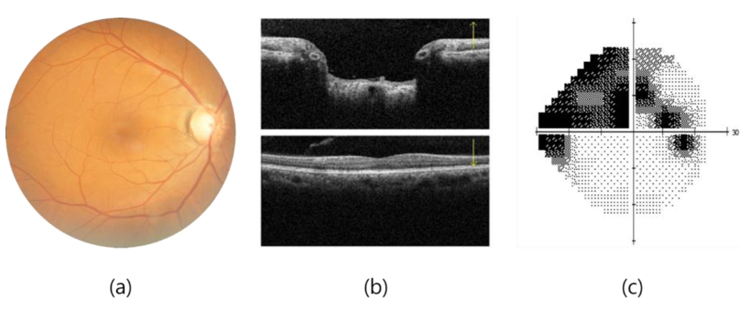
Glaucoma, which can cause irreversible visual impairment, is a widespread eye disease known as the “Invisible Vision Killer” due to its lack of noticeable symptoms in the early and middle stages, making it difficult to detect [1]. Glaucoma is anticipated to impact an increasing number of individuals globally because of an aging population [2,3,4]. The clinical diagnosis of glaucoma is achieved through various methods, such as fundoscopy, optical coherence tomography (OCT), and visual field examination, as shown in Figure 1. OCT offers high-resolution information on the thickness of the cornea, retina, and optic nerve, but the importance of the thickness of the ganglion cell complex (GCC) in diagnosing glaucoma remains a matter of debate [5]. A visual field examination can detect glaucoma when more than 40% of the optic nerve is damaged, resulting in changes in the visual field that threaten vision as they develop from the periphery, invade the center of the visual field, and advance. POAG, more prevalent in Westerners, leads to a gradual loss of vision, while PACG, more common in Easterners, causes rapid intraocular pressure increases, resulting in symptoms such as halo, blurred vision, severe eye pain, and nausea. Early screening is essential to prevent irreversible visual impairment.

Due to the superior image recognition capabilities of deep learning models, the medical field is increasingly using them to improve diagnosis accuracy and enhance human-machine collaboration. However, the lack of interpretability of early studies treating deep learning models as black boxes poses challenges in validating their effectiveness in clinical applications. To overcome this issue, researchers are using feature visualization methods to analyze deep learning models’ features and propose interpretable AI research that aligns with domain knowledge. The goal is to improve the reliability and acceptance of deep learning models for clinical applications.

The objective of this study is to train deep learning models on the NTUH Dataset fundus image dataset using four distinct approaches in order to analyze their impact on the model’s performance in measuring glaucoma. These approaches include:

(a)

obtaining two versions of fundus images using different fundoscopic angles, namely disc-centered (CD) on the optic disc (CD Fundus) and macular as the center (CM), termed CM Fundus,

(b)

using different cropping ratios to focus on smaller areas centered on the optic nerve disc (CD Crop) or macula (CM Crop) compared to the entire optic nerve disc-centered image,

(c)

applying various dataset splitting methods to divide patients into training, verification, and testing sets using different ratios, and

(d)

integrating the macular ganglion cell complex (GCC) thickness information with the fundus image for training the model.

After evaluating the impact of various network training methods on glaucoma diagnosis, this experiment will be repeated using the optimal method for both complete and cropped images of CD and CM. Moreover, two different visualization techniques, namely model-dependent CAM and model-independent LIME, will be utilized in this study to assess the areas of interest detected by the network models and verify their consistency with clinical diagnostic expertise.

This manuscript proposes three hypotheses, which will be tested through the following methods:

(a)

Investigating whether the deep learning model can detect subtle differences in the shape of the macular area, which are difficult to observe with the naked eye, in addition to the differences in the optic disc area observed in general clinical diagnosis, to test the ability of the model in interpreting glaucoma through fundoscopy.

(b)

Verifying whether the deep learning model reflects the changes in GCC cell layer thickness in the macula corresponding to glaucoma-induced optic nerve atrophy in fundoscopic image interpretation and determining whether the features learned from the model in the dataset have clinical reference value and testing whether the model reflects these changes.

(c)

Identifying the factors responsible for the high accuracy of deep learning models on fundoscopic images and ensuring the validity of AI models for clinical applications.

2. AI Interpretable and Visualization Techniques

Artificial intelligence has become an integral part of various industries, including finance, justice, and healthcare. While some AI applications, such as advertising recommendation systems, do not require transparency in decision-making, others, such as clinical diagnosis, demand interpretability. In healthcare, the results of an AI model can heavily influence important decisions, such as identifying the nature of a patient’s tumor. In such cases, if the model operates as a “black box,” i.e., lacking transparency, it becomes challenging to validate its effectiveness in clinical diagnosis. Focusing solely on achieving high accuracy without an explanation to justify the model’s decision-making process could undermine its clinical acceptance and reliability, leaving professional physicians hesitant to replace their diagnosis with an unverifiable AI system.

Explainable AI (XAI) is crucial in enhancing the transparency and efficacy of AI models and establishing trust in their use by domain experts. The focus of XAI research is primarily on developing methods that enable humans to comprehend the decision-making processes of AI systems.

Samek et al. [6] identified four key aspects of verifying, improving, learning from, and ensuring compliance with legislation to enhance the effectiveness and trustworthiness of AI systems. Christoph Molnar [7] classified model interpretation methods based on their local or global interpretability. Local interpretability pertains to understanding the behavior of an individual sample or a group of samples. As models become more accurate, they also become more complex, making it challenging for humans to comprehend the relationship between features and outcomes. In the following sections, we will discuss two methods for interpretability: the model-independent LIME method [8] and the model-dependent feature visualization CAM method [9].

2.1. Local Interpretable Model-Agnostic Explanation (LIME)

LIME, proposed by M. T. Ribeiro et al. in 2015 [8], is a model-independent technique for regional interpretability. By perturbing the input data of a network model, LIME identifies the input features that have the most influence on the model’s output. For instance, in the case of the Titanic passengers, numerical fields can be perturbed to comprehend which input features had a significant impact on whether the passengers survived the shipwreck. Today’s deep learning models offer high accuracy but have complex structures that make it challenging to explain their decision-making process. LIME is designed to address this problem by training a simple linear model that approximates the complex model and provides regional interpretability.

Figure 2 illustrates an interpretable area in the form of a concept map. The blue and red regions represent two categories of a complex classification model. Samples predicted within the red region are classified as “+”, while those in the blue region are classified as “●”. It is difficult to use a linear model to explain the behavior of the entire area of a complex model. However, if we focus on a specific area, a linear model can be used to fit the regional behavior of the complex model in that area. For instance, the thick red cross sample in Figure 2 can be utilized to interpret the deep learning model regionally by taking perturbation samples around it, classifying these samples using the original complex model, and training a simple linear model, such as the black dashed line. This enables the use of locally interpretable models for regional interpretation of deep learning models.

2.2. Class Activation Mapping (CAM)

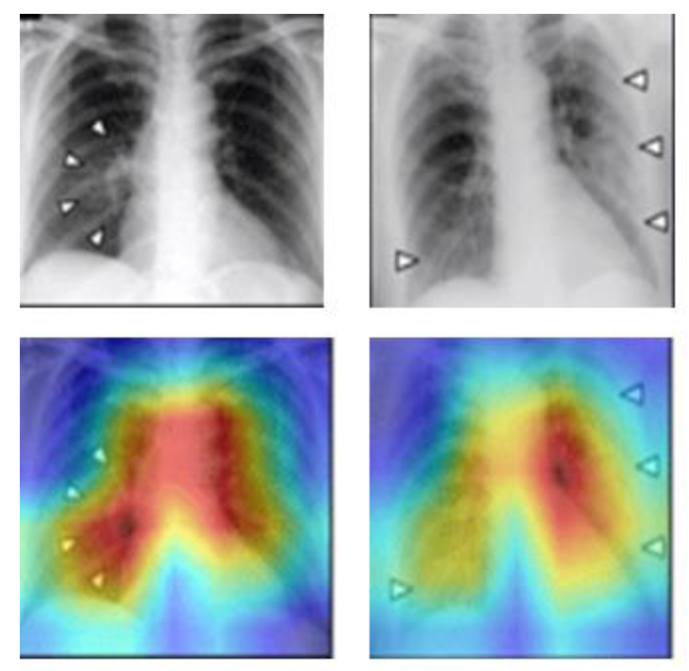
CAM is a CNN visualization technique introduced by B. Zhou et al. at the CVPR 2016 conference [9]. It was originally proposed to solve the problem of weakly supervised learning, where CNNs are capable of detecting and localizing objects even if they lack labeled location information during training. This ability is lost when the network uses the Fully Connected Layer, but replacing it with the Global Average Pooling (GAP) layer preserves the localization ability and reduces the overall network parameters. The CAM method can visualize the CNN network’s position of interest in classification and generate a heatmap for the overall object localization of the network. By combining CAM and GAP, the CNN can classify the image and locate specific areas related to the classification. For example, Figure 3 demonstrates the CAM schematic, where the CAM helps to identify the critical regions that need to be detected to diagnose COVID in the chest X-ray images.

3. Glaucoma Detection Based on Deep Learning

A. Diaz-Pinto et al. in 2019 used five different CNN architectures to evaluate the performance of glaucoma detection [10], in which the authors concluded that previous automated detection algorithms were highly dependent on the use of optic nerve disc and optic nerve cup segmentation for subsequent glaucoma determination, including focusing only on the segmented optic nerve cup or optic nerve disc. In their study on glaucoma detection, the authors compared the performance of five CNN [11] architectures, namely VGG16, VGG19, InceptionV3 [12], ResNet50 [13], and Xception [14], without relying on the cup-to-disc ratio (CDR) calculation or optic nerve disc and cup segmentation. The authors argued that as CNNs can learn discriminative features from images, it is not necessary to use CDR or optic nerve segmentation for glaucoma determination. The authors utilized pre-trained ImageNet weights for transfer learning, and the experimental results indicated that Xception outperformed VGG16 and VGG19 in terms of computational cost and accuracy. However, the incorrect judgment could be due to the absence of a larger bright area in the glaucoma image or the poor quality of the input image.

When testing CNNs on various public datasets, it was discovered that they did not perform well in terms of generalization to different datasets. This may be due to varying annotation standards across different datasets, such as experts making decisions based on different factors, including the patient’s medical history and fundus image, versus solely using the fundus image, resulting in less strict decisions and potentially leading to more false annotations.

In 2019, S. Phene et al. [15] proposed a CNN-based system for glaucoma detection and observation of optic nerve papillae features. They used an InceptionV3-based CNN architecture to train and evaluate color fundus images for glaucoma detection [14]. Their system provided good performance with higher sensitivity than ophthalmologists and comparable specificity to ophthalmologists. The authors emphasized the importance of fundus imaging, which is still the most commonly used low-cost medical imaging modality for evaluating ONH structures worldwide, especially in economically disadvantaged or medically underfunded areas. They also noted that there is no specific standard for deep learning to detect glaucoma on fundus images, and the clinical value of these systems is limited by differences in standards. To address this issue, the authors developed a system that could observe the features of interest to the model in detecting glaucoma as a way to assess the similarity between the features of interest to the ophthalmologist and the system. The results showed that the system mainly observes features such as a cup-to-disc ratio greater than 0.7 and RNFL impairment, which are the same decision areas of interest to ophthalmologists. By examining a single ONH feature, it is also possible to better understand which features the model’s predictions depend on.

In 2020, M. A. Zapata et al. [16] proposed a CNN-based glaucoma detection system that utilized five CNN models for various functional classifications. These included differentiating fundus images from other unrelated images in the dataset, selecting good-quality fundus images, distinguishing right eye (OD) and left eye (OS) in fundus images, detecting age-related macular degeneration (AMD), and detecting glaucomatous optic neuropathy. The model for detecting glaucoma was based on ResNet50 and mainly focused on observing the cup-to-disc ratio in the optic nerve disc region, along with some typical changes of glaucoma, such as RNFL defects. The authors also noted that non-mydriatic cameras (NMC) have become more popular for screening ophthalmic diseases using fundus imaging, which makes it a cost-effective approach. Incorporating AI into complementary diagnostic systems can also significantly reduce labor and time costs associated with image analysis. Furthermore, CNN can also be applied to other ophthalmic diseases, including AMD. Additionally, AI has the potential to observe information on fundus images that cannot be detected by the human eye, such as gender, age, and smoking status.

In 2019, S. Phan et al. [17] presented a glaucoma detection system for fundus imaging that utilized three different CNN architectures, namely VGG19 [11], ResNet152 [13], and DenseNet201 [18], to evaluate its performance and identify the region of interest for glaucoma diagnosis. The authors also employed a visualization technique called CAM to observe the identified region. The results demonstrated that the optic nerve disc was the primary area of observation for glaucoma diagnosis.

Similarly, in 2019, H. Liu et al. [19] proposed a CNN-based fundus imaging glaucoma detection system that utilized a ResNet lite version of GD-CNN [13]. The study not only evaluated the model’s performance but also incorporated visualization of the output heat map for observation purposes. The findings showed that the model correctly identified ONH lesions, RNFL defects, and localized defects.

In 2020, R. Hemelings et al. developed a CNN-based glaucoma detection system for fundus imaging that employed an active learning strategy and utilized ResNet50 for migratory learning. The model utilized uncertainty sampling as an active learning strategy, and the authors generated a significant map of the output model to observe the regions of concern and decisions made by the model. The authors found that the upper and lower edges of the optic nerve head (ONH) and the regions outside the ONH (the S and I regions in the ISNT principle) were relevant to the retinal nerve fiber layer (RNFL).

Also in 2020, F. Li et al. [20] proposed a CNN-based glaucoma detection system that used ResNet101 architecture and incorporated patient history information in the final fully connected layer. The model’s main concerns were identified using heatmaps generated by blocking tests, which revealed that the model focused on the edge of the ONH in non-glaucoma cases and on the area of RNFL defects above and below the ONH in glaucoma cases.

In 2021, R. Hemelings et al. [21] proposed another CNN-based glaucoma detection system using ResNet50 architecture, which aimed to address the lack of interpretability and decision transparency in deep learning glaucoma detection studies. The authors employed different cropping strategies to select 10–60% of the area centered on the ONH for cropping and removal, and the schematic for this cropping strategy is shown in Figure 4. Although most deep learning glaucoma detection studies exhibit high sensitivity and specificity, their lack of interpretability limits their clinical contribution.

The interpretability of CNNs is crucial for medical diagnosis [22,23] and building trust among experts. The authors note that it is unclear to what extent the information provided outside the ONH region on fundus images is relevant to glaucoma at this stage of research. To better analyze the feature information provided by the ONH and outside the ONH region, the cropping strategy excludes both the ONH region and the area outside it. The experimental results demonstrate that the deep learning model can identify the presence of glaucoma in areas outside the ONH of the fundus image. Additionally, a significant map experiment was conducted with various cutting strategies. The results, depicted in Figure 5, indicate that the model’s attention is mainly on the ONH region for glaucoma detection. As the area removed by cutting increased, the model’s attention was mainly on the upper (S) and lower (I) regions in the ISNT principle outside the ONH, which is the thickest area of RNFL in the retina. The final experimental results also demonstrate that the trained glaucoma model can detect and use the subtle changes in the RNFL that are not visible to the human eye.

4. Materials

The NTUH dataset used in this paper was retrospectively collected by the NTUH team and contains two types of images for each patient: funduscopic images and optical homogeneous tomography (OCT) images. The OCT images provide information on the thickness of the RNFL layer under the optic disc area and the thickness of the GCC layer under the macula area. Figure 6 shows an example of the dataset, where (a) is the funduscopic image, (b) is the OCT image corresponding to (a), and (c) is the thickness information of the GCC layer corresponding to (b). The funduscopic image and the GCC layer thickness information were primarily used for the research experiment.

4.1. Fundoscopic Images

A total of 610 ophthalmology patients were included in the study, comprising 326 non-glaucoma patients and 284 glaucoma patients, with both right and left eye images collected. The distribution of fundus images is presented in

Table 1. Distribution of fundus imaging among patients.

Type	No. of Patient	Eye Type	No. of Images
Non-Glaucoma	326	OD	326
		OS	322
Glaucoma	284	OD	275
		OS	284

. The dataset consisted of 1207 images, which were captured using two framing types. Figure 7 illustrates the 1207 images with the optic nerve disc as the center (CD), while Figure 8 shows the 1207 images with the macular as the center (CM).

4.2. GCC Layer Thickness Information Images

The GCC layer thickness information images in this study consist of 1207 images that correspond to the macular region of the patients’ eyes in the NTUH dataset. These images were generated by cropping the GCC thickness information from the optical homogeneous tomography report and are sized at 560 pixels long and 570 pixels wide. The degree of GCC damage is categorized and color-coded in

Table 2. Color and range values for GCC with different thickness grades.

Thickness Grade Distance	Definition	Representative Color
>5%	Normal range	Green
<5%	Critical value	Yellow
<1%	Below normal range	Red

, while Figure 9 displays examples of GCC layer impairment and Figure 10 shows examples of the GCC layer in a healthy state.

5. Proposed Method

The main objective of this study is to investigate the differences in the macular region of glaucoma, and ResNet50 was chosen as the network architecture without any specific classification model enhancements. The study’s system architecture, shown in Figure 11, is composed of four sections: data pre-processing, model training, network performance evaluation, and CAM visualization and LIME area interpretability. The subsequent sections of the paper will provide further details on each section. To avoid the model learning irrelevant features, such as time stamps and missing corners used for identifying different instrument brands, these features were removed from the original instrument output. Furthermore, to ensure that left and right eyes were evenly distributed in the entire dataset, a random horizontal flip was used with a 0.5 rate to perform data augmentation. The fundoscopic images were categorized into right eye (OD) and left eye (OS) based on the patient’s eyes.

6. Model Training and Evaluation

This paper utilizes ResNet50 as the backbone of the deep learning network to effectively use high- and low-dimensional feature data. Four different experiments were designed to analyze the impact of features provided by each method on the network model’s determination performance for images in the NTUH dataset. These experiments include different fundus lens angles, varying cropping ratios of fundus images, importing macular ganglion cell complex (GCC) thickness information, and different dataset slicing methods, which will be discussed in subsequent sections.

Different Disc Positions

The impact of different features on the network model’s performance is analyzed by collecting fundus images with various disc positions, as shown in Figure 12.

To investigate the impact of different extracted features on model performance, several cropping scales are used in this study, as shown in Figure 13.

The NTUH dataset was divided into four categories based on the glaucomatous condition and the thickness of the GCC layer. Category 1 and 4 were used as positive and negative samples for the training process, as shown in Figure 14.

To ensure a fair and rigorous performance evaluation, the data split was conducted based on patients rather than fundus images. Using the ratio of 6:2:2 for training, validation, and testing datasets is more rigorous and consistent because it ensures an equal number of samples for both validation and testing, resulting in a fair evaluation of the model’s performance.

7. Features Analysis and Explainability

In the upcoming sections, we will explain how to use different methods to visualize and improve the interpretability of the models. To improve the interpretability, two methods—CAM visualization and LIME region interpretability—will be applied to models with the highest accuracy obtained from various methods. These methods will be discussed in detail in the subsequent sections.

7.1. CAM Visualization

In the CAM section, the ResNet50 model framework is used to extract the results of 2048 depth features from the AvgPool layer. The discrimination power of each depth feature is calculated using a decision stump to distinguish between glaucoma and non-glaucoma categories. The top 100 features representing these categories are selected based on their ranking, as shown in Figure 15, and their classification results in all fundus images for glaucoma and non-glaucoma categories are obtained with confidence. The top 200 fundus images in each category with the highest match for each feature are ranked and output as a heatmap. This helps to identify the areas of fundus imaging that are most important for determining glaucoma. Additionally, the GCC thickness information is compared to explain the model’s prediction, identify areas of interest, and correlate them with clinical domain knowledge.

7.2. LIME Local Interpretability

The fundus images were sliced using Super-Pixels, and the trained ResNet50 network model was perturbed to take samples. The perturbed samples were fed into the network model for prediction to train a linear model, and the behavior of this linear model at the sample points would be similar to the original deep learning model. The trained linear model is then used to predict the sample, obtain the classification results and confidence level of each fundus image for glaucoma and non-glaucoma, and then obtain and rank the top 100 images with the highest confidence level for glaucoma and non-glaucoma, respectively. There are two circumstances: the top 1, 3, and 5 positive or negative area maps, or the top 10 area maps with both positive and negative areas, as shown in Figure 16. The positive area means that the network will judge the whole image as a plus-decision area of that category, which is marked in green; the negative area means that the network will judge the whole image as a minus-decision area of another category, which is marked in red; the area mentioned here is the area obtained by slicing the fundus image using Super-Pixels. Finally, the positive and negative region maps were superimposed on the original fundus images, and the output region maps were observed for the regions of interest or major decision areas for different classification results. They were then further compared with the GCC thickness information or clinical diagnosis experience to explain why the model made the prediction and which regions were looked at, corresponding to the clinical domain knowledge.

8. Experimental Results

In this section, comprehensive experiments are conducted to understand the impact of different disc portions, crop sizes, and GCC thickness information, along with detailed ablation studies. A CAM visualization is also performed to understand the significance of the proposed model.

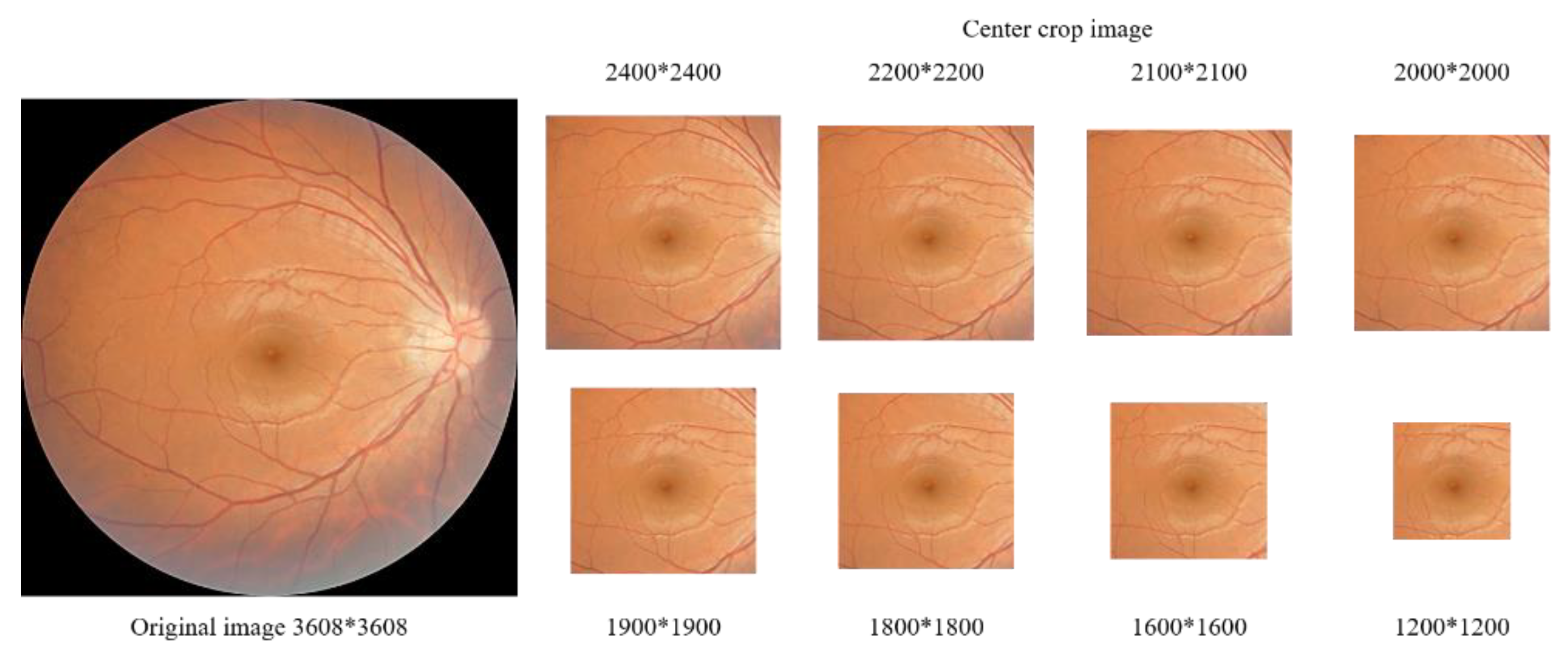
8.1. Different Disc Positions and Crop Sizes

The experiments using different fundoscopic angles, as listed in

Table 3. Performance scores for different features of CD, CM, and the two combined.

Dataset	Accuracy	Sensitivity	Specificity	Precision	F1-Score
CD + CM	0.863	0.839	0.883	0.862	0.850
CD	0.823	0.800	0.843	0.814	0.807
CM	0.857	0.781	0.921	0.895	0.834

, showed that CM alone had an accuracy of 85.7% and focused more on learning non-glaucoma features based on specificity results. Further observation of features provided by CD and CM through fundus images with different cropping scales was deemed necessary. Experiments with different crop sizes, as listed in

Table 4. Performance scores for different crop sizes.

Dataset	Accuracy	Sensitivity	Specificity	Precision	F1-Score
CD (Crop 1200)	0.831	0.800	0.859	0.830	0.814
CD (Crop 1800)	0.823	0.781	0.859	0.826	0.803
CM (Crop 1200)	0.764	0.800	0.734	0.721	0.758
CM (Crop 1800)	0.790	0.745	0.828	0.788	0.766

, revealed that the macular area alone had an accuracy of 79%, and the accuracy of different cuts of the optic disc area alone was also higher than that of the macular area alone, which aligns with clinical diagnosis. CM cuts, which excluded the optic disc area, achieved an accuracy of 76.4% or better, indicating that the macular region provides sufficient non-robust features for representing the presence or absence of glaucoma.

8.2. GCC Thickness Information

Table 5. Performance scores for the CM and GCC combination for Type 1 data.

Dataset	Accuracy	Sensitivity	Specificity	Precision	F1-Score
CM + GCC	0.908	0.921	0.893	0.903	0.912

shows the experimental results of using the GCC thickness information method, which improved the accuracy to 90.8%. This suggests that the model can more easily learn about the characteristics of glaucoma by avoiding errors or other complications in the OCT instrument output. However, since Type II and III images were excluded from the test, the results may be less rigorous and more biased. To address this issue, the network model was further tested using a set of CM images without GCC thickness information.

Table 6. Performance scores with and without GCC, including all types.

Model	Dataset	Accuracy	Sensitivity	Specificity	Precision	F1-Score
CM	CM	0.834	0.777	0.885	0.857	0.815
CM + GCC	CM	0.870	0.926	0.820	0.820	0.870

shows that the model with GCC thickness information had about 4% higher accuracy than the model without it. Fundus images can provide information on GCC layer damage in addition to glaucoma characteristics, and the model was found to be affected by the presence or absence of GCC layer damage.

8.3. GCC Partitioned by Patients

The results of the experiments using GCC partitioned by patients are shown in

Table 7. Performance scores using the CM and GCC combination for patient and image-based data.

Dataset	Accuracy	Sensitivity	Specificity	Precision	F1-Score
CM + GCC (By Patients)	0.863	0.893	0.812	0.893	0.893
CM + GCC (By Images)	0.908	0.921	0.893	0.903	0.912

. From the experimental results, it can be seen that patient-based data set slicing can avoid bias in the determination and thus obtain a more rigorous performance evaluation.

8.4. Different Ratios

Table 8. Performance scores using the CM and GCC combination for different ratios.

Dataset	Accuracy	Sensitivity	Specificity	Precision	F1-Score
CM + GCC + Person (7:2:1)	0.863	0.893	0.812	0.893	0.893
CM + GCC + Person (6:2:2)	0.893	0.882	0.905	0.909	0.895

presents the results of experiments with different data set slice ratios. When using a ratio of 6:2:2 for training, validation, and test sets, as compared to a ratio of 7:2:1, the results were more rigorous, with an accuracy of 89.3% and a more balanced sensitivity and specificity. This is because the number of validation and test sets was equal, leading to a more reliable evaluation of the model’s performance.

8.5. Ablation Test

Based on the experimental results of various experiments in the previous sections, the aim of this study is to evaluate the effect of adding different methods on the network model’s performance and accuracy, so the ablation test was planned. The test set used in this experiment is fixed to the original CM test set without any further processing. The results of the ablation experiment are shown in

Table 9. Performance scores for different CM, GCC, and person combinations.

Model	Dataset	Accuracy	Sensitivity	Specificity	Precision	F1-Score
CM	CM	0.857	0.781	0.921	0.895	0.834
CM + GCC	CM	0.870	0.926	0.820	0.820	0.870
CM + GCC + Person	CM	0.930	0.981	0.885	0.883	0.930

.

8.6. Complete Experiments with CD Fundus Images

The complete experimental results for CD are shown in

Table 10. Detailed results for different CD, GCC, and person combinations with varying crop sizes.

Dataset	Accuracy	Sensitivity	Specificity	Precision	F1-Score
CD + GCC + Person	0.893	0.873	0.915	0.918	0.894
CD (Crop2400) + GCC + Person	0.908	0.863	0.957	0.957	0.907
CD (Crop2200) + GCC + Person	0.867	0.843	0.894	0.896	0.869
CD (Crop2100) + GCC + Person	0.867	0.794	0.947	0.942	0.862
CD (Crop2000) + GCC + Person	0.903	0.873	0.936	0.937	0.904
CD (Crop1900) + GCC + Person	0.893	0.892	0.894	0.901	0.897
CD (Crop1800) + GCC + Person	0.862	0.794	0.936	0.931	0.857
CD (Crop1600) + GCC + Person	0.878	0.804	0.957	0.953	0.872
CD (Crop1200) + GCC + Person	0.908	0.882	0.936	0.938	0.909

. The accuracy of the trained network model for determining the presence of glaucoma was almost the same for both the full image and the optic nerve disc-centered fundus image at various crop scales. Whether or not the model pays more attention to the optic disc area makes little difference to the final result.

8.7. Complete Experiments with CM Fundus Images

The complete experimental results for CM are shown in

Table 11. Detailed results for different CM, GCC, and person combinations with varying crop sizes.

Dataset	Accuracy	Sensitivity	Specificity	Precision	F1-Score
CM + GCC + Person	0.898	0.882	0.915	0.918	0.900
CM (Crop2400) + GCC + Person	0.867	0.804	0.936	0.932	0.863
CM (Crop2200) + GCC + Person	0.898	0.882	0.915	0.918	0.900
CM (Crop2100) + GCC + Person	0.872	0.824	0.926	0.923	0.870
CM (Crop2000) + GCC + Person	0.867	0.863	0.872	0.880	0.871
CM (Crop1900) + GCC + Person	0.821	0.696	0.957	0.947	0.802
CM (Crop1800) + GCC + Person	0.837	0.755	0.926	0.917	0.828
CM (Crop1600) + GCC + Person	0.832	0.765	0.904	0.897	0.825
CM (Crop1200) + GCC + Person	0.806	0.775	0.840	0.840	0.806

. The accuracy of the trained network model in determining the presence of glaucoma decreases as the cropping area becomes smaller and more attention is paid to the macula and its surrounding area, using either the full image or a fundus image centered on the visual macula at various cropping scales. However, the minimum is more than 80.6%, and after the crop size range is below 2000, the fundus image almost only includes the macula and its surrounding area, which can exclude the influence of the optic disc. The results of the sensitivity and specificity experiments showed that the model at this time focused more on the health characteristics of non-glaucoma patients in determining whether glaucoma was present.

8.8. Comparison of CD and CM Complete Experiments

The accuracy of the complete experimental results of CD and CM was further organized into a table for direct comparison and evaluation, and the comparison table of experimental results is shown in

Table 12. Detailed results for different CD and CM with varying crop sizes.

Dataset	CD Accuracy	CM Accuracy
No Crop	0.893	0.898
Crop 2400	0.908	0.867
Crop 2200	0.867	0.898
Crop 2100	0.867	0.872
Crop 2000	0.903	0.867
Crop 1900	0.893	0.821
Crop 1800	0.862	0.837
Crop 1600	0.878	0.832
Crop 1200	0.908	0.806

. The CM part of the results is shown in red, which means that the fundus images used in the training of the model contain almost only the macula and its surrounding area, which can exclude the effect of the optic disc.

In the comparison of the experimental results, it can be found that whether the training images are used in full or in part, the final judgment result is not affected by the use of the visual plexus area. This part is also consistent with the clinical diagnostic experience, and it means that the models are learning whether robustness features represent glaucoma or not. In the case of the macular region only, although the accuracy of the results is reduced due to the exclusion of the optic disc and its region during training, it is not so reduced that the results are not credible or have no reference value for determining whether glaucoma is present. However, it is not easy to focus on specific features in the macular region on the fundus image with the naked eye clinically, indicating that the model can actually learn through the macula and its surrounding area what the human naked eye cannot detect and observe enough non-robust features to represent glaucoma.

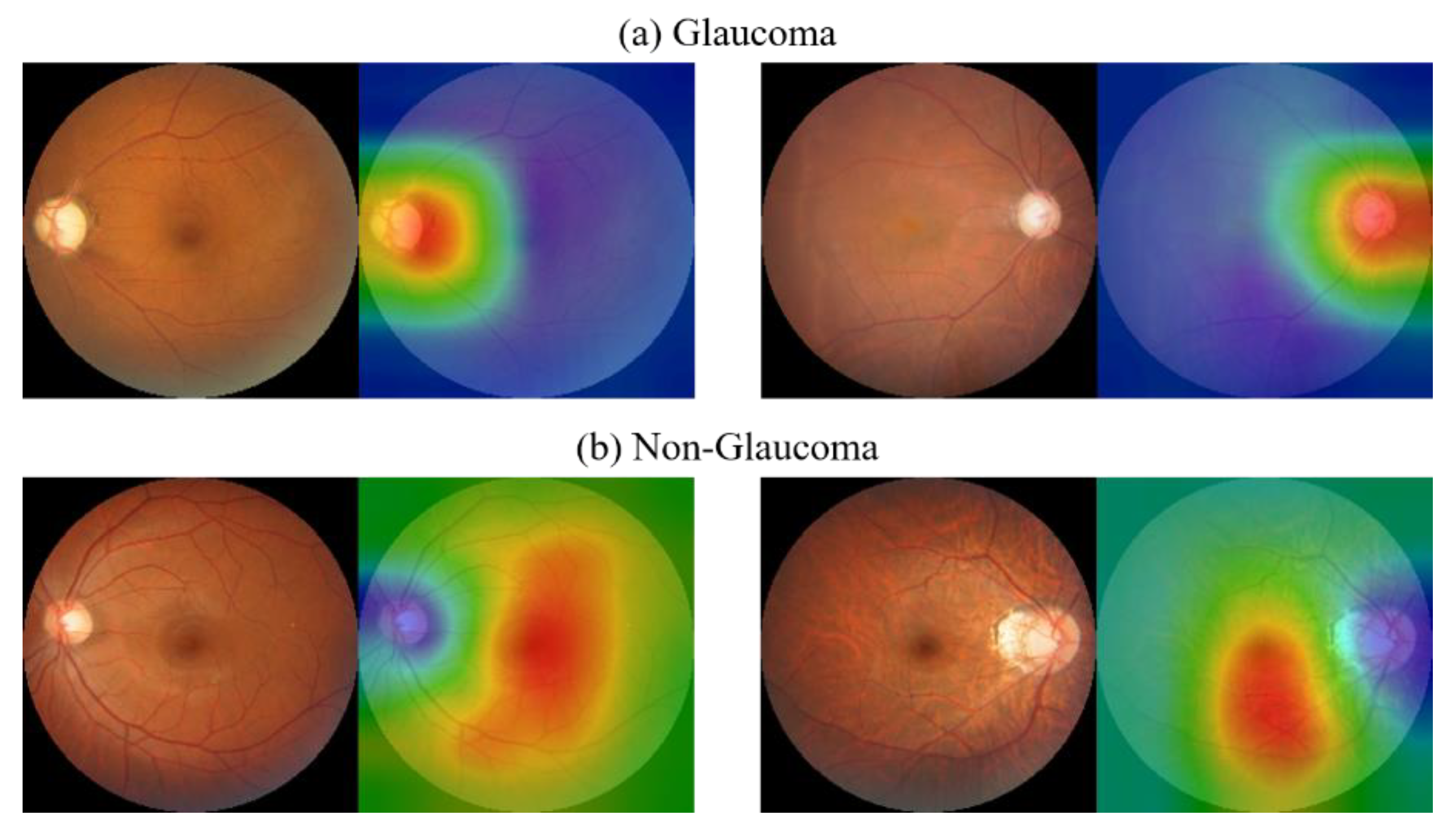
8.9. CAM Visualization

The results of the CAM analysis for two categories are shown in Figure 17. From the results of the CAM experiment of CM images, it can be found that when the images are judged as glaucoma, the area of greatest concern for the model is the optic disc area, and this part is also consistent with the clinical diagnosis experience. In non-glaucoma cases, the opposite result was found as in glaucoma cases, where the model focused on all areas except the optic disc, with emphasis on the macula and its surrounding areas.

The first and second most discriminating features are further extracted from the heatmap and compared with the GCC thickness map. It can be found that the areas of interest and structure of the model are to some extent similar to the damaged areas of the GCC layer. Discriminative features are visualized as shown in Figure 18. This again validates the model’s ability to observe subtle non-robust features on the macula and its surrounding areas, as well as providing information on GCC layer damage and the relevance of GCC layer damage to the development of glaucoma after incorporating GCC thickness information.

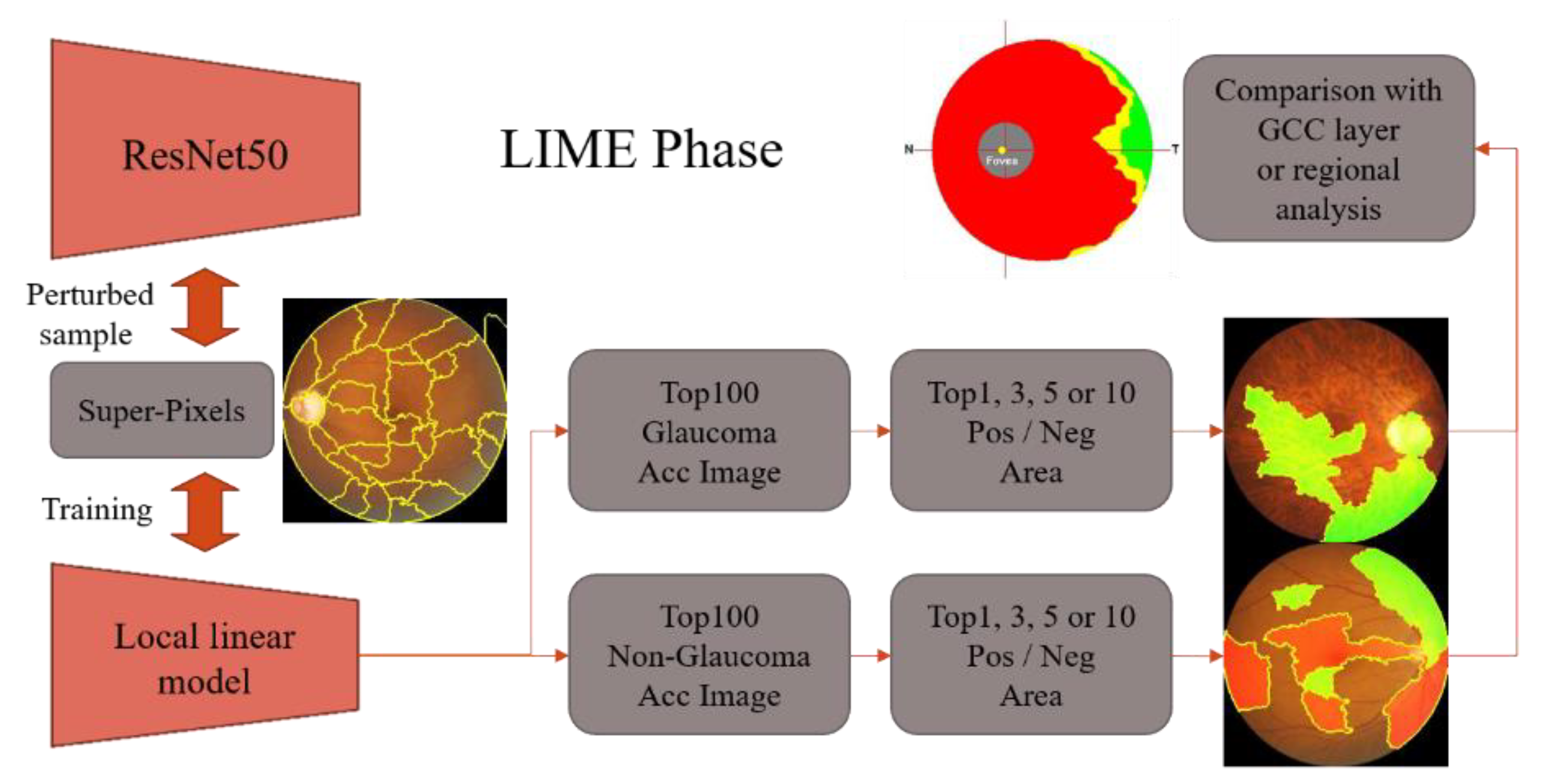
8.10. LIME Visualization

The results of the LIME analysis for two categories are shown in Figure 19. When the image is determined to be glaucoma, the first 10 areas of the image are all green positive areas (glaucoma plus areas), and the positive areas all contain the optic disc itself. When the image is determined to be non-glaucoma, one or more red negative areas begin to appear in the top 10 areas of the image, and the red areas then contain the optic disc itself. Because of the Super-Pixel approach, the top 10 regions are a bit too extensive to be observed simultaneously. In order to arrive at a more precise explanation, the experiment further analyzes the positive and negative regions of the top 1 and top 3 in each case. The results of the LIME analysis for two categories are shown in Figure 20.

Based on the LIME visualization outcomes for the top 1 and top 3, it is apparent that the areas of interest for glaucoma and non-glaucoma are contrasting. Moreover, it can be inferred that when identifying glaucoma, the optic disc area is the primary focus, while for non-glaucoma, the emphasis is not on the optic disc area but on the macula and its surrounding region.

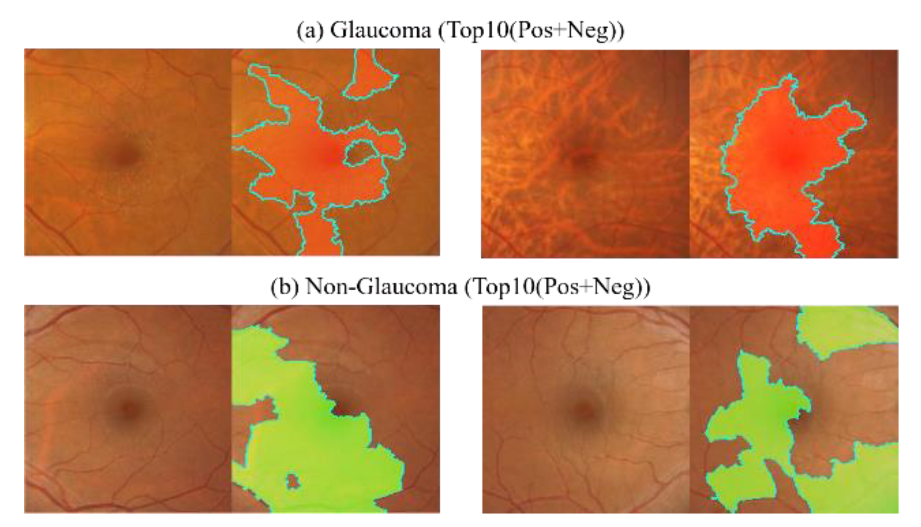
The experimental findings using the 1800 × 1800 size CM fundus images with LIME for the top 10 positive and negative decision areas differ from those obtained using full CM images, as shown in Figure 21. This difference can be attributed to the exclusion of the effect caused by the optic disc area in the cropped images.

The top 10 areas identified by the deep learning model as having the most significant impact on determining glaucoma or non-glaucoma are primarily focused on the macula and its surrounding regions. However, a notable difference is observed in the top 10 glaucoma cases, where there are no positive areas of interest, indicating that negative areas are stronger features for glaucoma detection. On the other hand, the top 10 non-glaucoma cases are in the positive region, indicating that only fundus images of the macula can collapse into a pattern to determine non-glaucoma cases. However, the macula alone may not provide enough features to determine the presence of glaucoma, but it can help determine the absence of glaucoma. As both results are extreme, the study further analyzes the positive and negative regions for the top 1 and top 3 cases in each category, as shown in Figure 22. The LIME analysis of the two categories is also presented in the figure.

The LIME visualization results for the top 1 and top 3 showed that the areas of interest for glaucoma and non-glaucoma were opposite to the results obtained using the entire CM image. However, when considering the top 10 glaucoma macular regions, LIME visualization was found to be stronger at identifying negative regions. Therefore, in glaucoma detection, more attention should be paid to the features that indicate non-glaucoma in the macular region, while in non-glaucoma detection, only the macular region should be considered without focusing on other surrounding areas.

9. Conclusions

This study aimed to investigate the performance and extracted features of deep learning models in glaucoma assessment using extensive experiments and two deep feature visualization methods. The goal was to improve the validity and robustness of the proposed AI-assisted system for glaucoma inspection and ensure that it aligns with clinical diagnostic rules. The experimental results not only demonstrated the consistency between deep learning models and clinical experience but also revealed the association between GCC defects in macular regions and glaucoma. The developed AI-assisted system for glaucoma inspection using deep learning frameworks can aid in early detection and reduce the possibility of missing detection, leading to timely treatment for glaucoma patients and preventing vision impairment.