
Application of Enterprise Architecture and Artificial Neural Networks to Optimize the Production Process

Abstract
:1. Introduction
2. Meta-Model of Enterprise Architecture
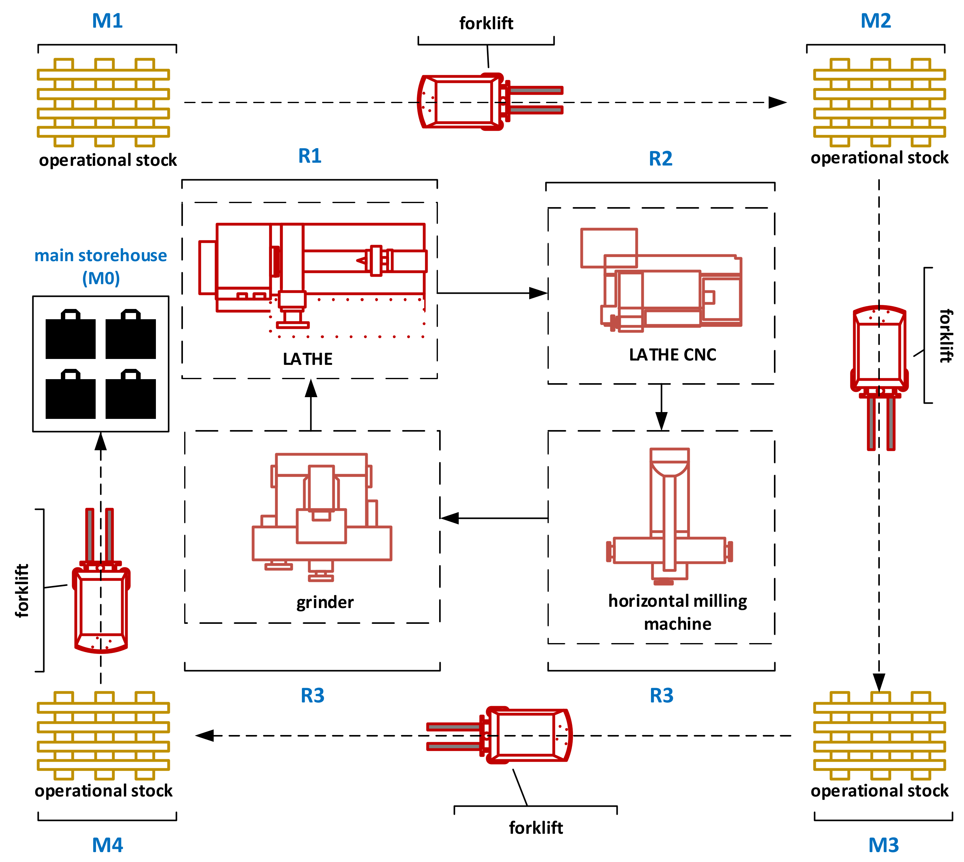
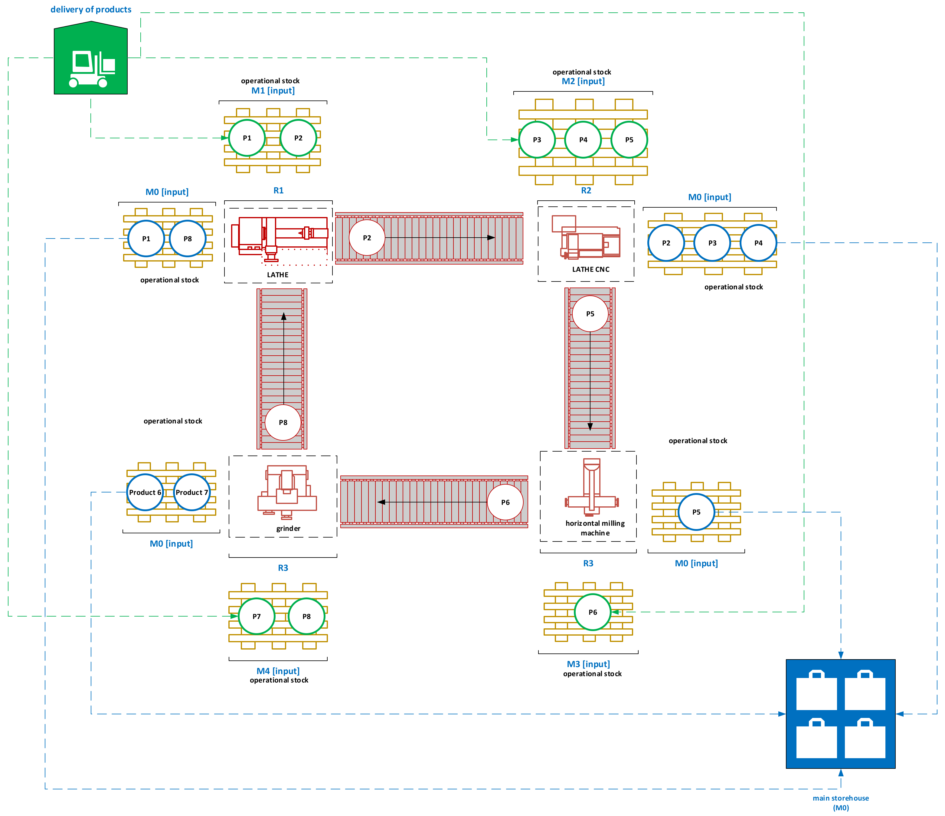
- —resources (all material and non-material elements of the production process that are necessary to produce products, e.g., machines, raw materials, employees, tools, etc.);
- —processes (all phenomena and deliberately undertaken actions which result in the gradual occurrence of the desired changes in the subject of work subject to their influence);
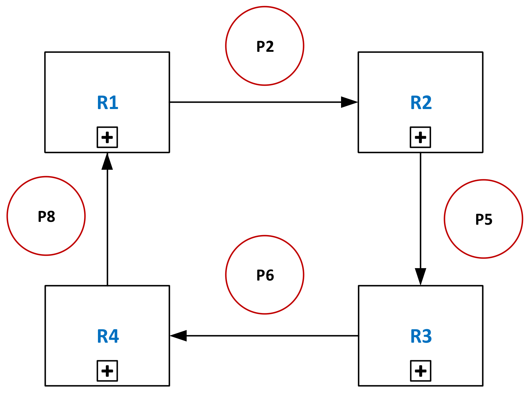
- —relationships (all connections and interdependent that affect the manufacture or maintenance of products or services).
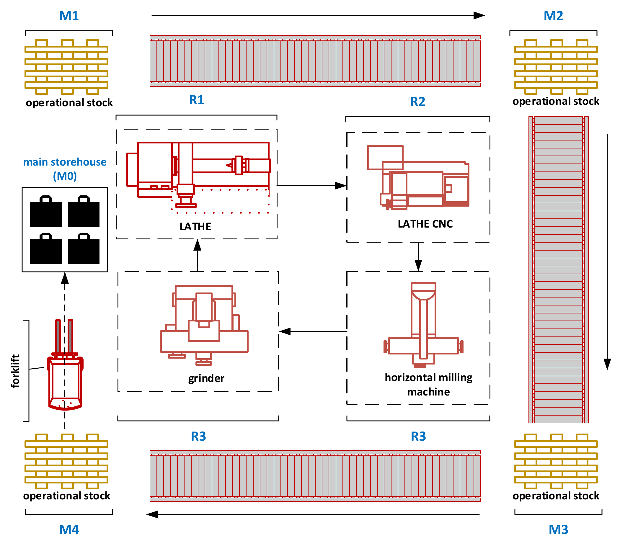
3. Illustrative Example of Production Process
- Q2: How to efficiently use the resources?
- Q3: What is the maintenance plan for ?
- Q4: How to minimize inventory?
4. Implementation Framework Using Enterprise Architecture
5. Formalizing a Mathematical Model of Production Planning, Maintenance and Resource Allocation
6. Computational Experiments
6.1. Evaluation Criterion
6.2. Developing a Training Pattern for ANN
6.3. Building an ANN
7. Conclusions
Author Contributions
Funding
Conflicts of Interest
Appendix A. Data for Experiment_1 and Experiment_2

| Record Number | |||||||||||||||
|---|---|---|---|---|---|---|---|---|---|---|---|---|---|---|---|
| 1 | 6 | 8 | 4 | 466,426 | 50 | 45 | 1 | 22 5 55 95 11 72 60 52 | 6 6 0 6 8 9 2 2 | 1 0 1 1 1 1 0 0 | 13 39 31 39 7 24 35 9 | 1 1 0 1 | 45 0 0 0 20 10 0 0 25 10 20 0 30 10 0 30 22 40 0 0 0 20 0 0 40 0 20 400 0 10 30 30 30 0 10 20 20 10 20 20 10 0 20 10 0 0 0 0 | 15 80 59 67 38 14 95 78 96 85 1 91 18 45 76 61 81 0 91 23 18 70 36 10 | 4 5 0 0 0 0 0 5 0 3 2 2 5 0 0 0 0 2 0 0 7 7 0 0 0 0 0 0 0 4 1 5 |
| … | |||||||||||||||
| 50 | 6 | 8 | 4 | 724,775 | 45 | 552 | 1 | 62 61 85 64 40 12 33 83 | 4 7 4 4 1 8 2 8 | 1 0 1 0 0 1 1 0 | 46 0 41 33 39 21 49 28 | 1 0 0 1 | 1 3 9 9 8 4 5 5 2 5 8 9 5 1 3 3 2 3 0 7 3 0 3 4 5 1 9 4 5 9 2 5 4 9 3 7 2 4 4 3 8 8 3 1 1 0 6 5 | 86 62 72 85 15 60 12 26 9 19 95 94 30 77 53 59 99 23 24 78 81 38 65 58 | 7 6 0 5 6 2 0 3 1 5 9 9 7 9 7 3 5 8 8 0 5 3 2 7 8 2 0 5 5 0 5 9 |
| Record Number | |||||||||||||||
|---|---|---|---|---|---|---|---|---|---|---|---|---|---|---|---|
| 1 | 6 | 8 | 4 | 368,888,888,000 | 1,800,000,000 | 2227 | 2 | 46 46 61 74 8 73 43 42 | 70 30 40 60 10 90 10 80 | 0 1 0 0 1 1 1 0 | 4 17 33 39 33 4 3 45 | 1 1 1 1 | 9 0 5 0 3 1 3 6 0 4 7 3 1 4 8 5 7 3 7 1 0 5 8 5 2 1 7 6 8 9 9 7 3 4 4 5 3 7 4 7 3 1 4 8 7 4 4 8 | 93 85 40 28 4 18 73 79 14 10 58 59 59 18 9 23 84 36 39 25 17 10 83 46 | 6 2 1 7 4 8 3 5 0 3 0 2 3 0 2 8 3 2 3 0 2 7 8 6 9 1 9 3 0 7 8 7 |
| … | |||||||||||||||
| 10 | 6 | 8 | 4 | 466,426 | 1,800,000,000 | 2227 | 2 | 46 46 6 74 80 730 400 420 | 70 300 400 600 10 900 100 800 | 0 1 0 0 1 1 1 0 | 4 17 33 39 33 4 3 45 | 1 1 1 1 | 9 0 5 0 3 1 3 6 0 4 7 3 1 4 8 5 7 3 7 1 0 5 8 5 2 1 7 6 8 9 9 7 3 4 4 5 3 7 4 7 3 1 4 8 7 4 4 8 | 93 85 40 28 4 18 73 79 14 10 58 59 59 18 9 23 84 36 39 25 17 10 83 46 | 6 2 1 7 4 8 3 5 0 3 0 2 3 0 2 8 3 2 3 0 2 7 8 6 9 1 9 3 0 7 8 7 |
| Record Number | Costs Storage | ||||
|---|---|---|---|---|---|
| 1 | t = 1 2 3 4 5 6 p1 0 0 0 0 0 3 p2 0 1 3 14 7 0 p3 5 9 1 0 0 0 p4 0 0 1 13 0 0 p5 40 1 22 42 0 10 p6 0 7 7 0 0 0 p7 20 10 20 20 10 0 p8 0 0 0 0 0 0 | t = 1 2 3 4 5 6 p1 44 0 0 0 20 7 p2 0 0 21 0 9 0 p3 24 1 0 29 22 40 p4 0 0 0 5 0 0 p5 0 0 0 354 0 0 p6 29 23 23 0 10 20 p7 0 0 0 0 0 0 p8 20 10 0 0 0 0 | t = 1 2 3 4 5 6 r1 0 1 1 1 1 1 r2 1 1 1 1 0 1 r3 1 1 1 1 1 1 r4 1 1 1 1 1 0 | r1 0 r2 0 r3 0 r4 0 | 431 |
| … | |||||
| 50 | t = 1 2 3 4 5 6 p1 2 0 2 0 0 0 p2 2 3 0 0 0 0 p3 1 4 1 0 7 3 p4 0 0 0 1 0 3 p5 1 1 2 5 0 3 p6 0 0 0 0 1 0 p7 4 0 0 0 0 0 p8 0 0 0 0 4 2 | t = 1 2 3 4 5 6 p1 7 0 3 0 3 1 p2 0 3 0 4 7 3 p3 0 0 7 5 0 0 p4 7 1 0 4 8 2 p5 0 0 5 1 8 6 p6 8 7 3 4 3 5 p7 0 5 4 7 3 1 p8 4 8 7 4 0 6 | t = 1 2 3 4 5 6 r1 1 1 1 1 1 1 r2 1 1 1 1 1 1 r3 1 1 1 1 1 1 r4 1 1 1 1 1 1 | r1 0 r2 0 r3 0 r4 0 | 6 |
| Record Number | Costs Storage | ||||
|---|---|---|---|---|---|
| 1 | t = 1 2 3 4 5 6 p1 0 0 0 0 0 0 p2 4 0 0 0 0 0 p3 6 12 0 0 7 3 p4 0 0 2 0 1 0 p5 9 0 0 5 0 6 p6 0 0 0 0 0 0 p7 2 0 0 0 0 0 p8 0 0 0 0 5 2 | t = 1 2 3 4 5 6 p1 9 0 5 0 3 1 p2 0 4 0 4 7 3 p3 0 0 0 0 0 0 p4 7 1 0 3 7 5 p5 0 0 0 1 8 3 p6 8 7 3 4 4 5 p7 0 7 4 7 3 1 p8 4 8 7 4 0 5 | t = 1 2 3 4 5 6 r1 1 0 1 1 1 1 r2 1 1 0 1 1 1 r3 1 0 1 1 1 1 r4 1 1 1 0 1 1 | r1 1 r2 1 r3 1 r4 1 | 1411 |
| … | |||||
| 8 | t = 1 2 3 4 5 6 p1 5 0 0 0 0 0 p2 0 1 0 0 0 0 p3 1 9 4 0 10 0 p4 0 0 0 0 1 5 p5 18 5 0 5 0 0 p6 0 0 0 0 0 0 p7 0 0 0 0 0 0 p8 0 0 0 0 4 0 | t = 1 2 3 4 5 6 p1 4 0 5 0 3 1 p2 2 5 0 4 7 3 p3 0 0 0 4 0 0 p4 7 1 0 5 7 0 p5 0 0 0 0 0 4 p6 8 7 3 4 4 5 p7 2 7 4 7 3 1 p8 4 8 7 4 0 8 | t = 1 2 3 4 5 6 r1 1 1 0 1 1 1 r2 1 1 1 1 1 0 r3 1 1 0 1 1 1 r4 1 1 1 0 1 1 | r1 1 r2 1 r3 1 r4 1 | 2607 |
| Record Number | |||||||||||||||
|---|---|---|---|---|---|---|---|---|---|---|---|---|---|---|---|
| 1 | 6 | 8 | 4 | 466,426 | 50 | 45 | 1 | 22 5 55 95 11 72 60 52 | 6 6 0 6 8 9 2 2 | 1 0 1 1 1 1 0 0 | 13 39 31 39 7 24 35 9 | 1 1 0 1 | 0 1 0 1 5 7 4 9 6 9 9 3 7 9 0 8 8 1 0 9 4 3 5 0 1 6 3 2 9 9 2 3 2 8 6 6 7 5 7 4 8 1 2 7 0 5 5 0 | 15 80 59 67 38 14 95 78 96 85 1 91 18 45 76 61 81 0 91 23 18 70 36 10 | 1 2 3 1 1 2 9 5 6 0 6 8 8 6 0 0 4 5 9 2 8 4 4 8 2 0 5 7 4 0 4 1 |
| … | |||||||||||||||
| 50 | 6 | 8 | 4 | 724,775 | 45 | 552 | 1 | 62 61 85 64 40 12 33 83 | 4 7 4 4 1 8 2 8 | 1 0 1 0 0 1 1 0 | 46 0 41 33 39 21 49 28 | 1 0 0 1 | 1 3 9 9 8 4 5 5 2 5 8 9 5 1 3 3 2 3 0 7 3 0 3 4 5 1 9 4 5 9 2 5 4 9 3 7 2 4 4 3 8 8 3 1 1 0 6 5 | 86 62 72 85 15 60 12 26 9 19 95 94 30 77 53 59 99 23 24 78 81 38 65 58 | 7 6 0 5 6 2 0 3 1 5 9 9 7 9 7 3 5 8 8 0 5 3 2 7 8 2 0 5 5 0 5 9 |
| Record Number | Classification Label | |||||||||||||||
|---|---|---|---|---|---|---|---|---|---|---|---|---|---|---|---|---|
| 1 | 6 | 8 | 4 | 466,426 | 50 | 45 | 1 | 22 5 55 95 11 72 60 52 | 6 6 0 6 8 9 2 2 | 1 0 1 1 1 1 0 0 | 13 39 31 39 7 24 35 9 | 1 1 0 1 | 0 1 0 1 5 7 4 9 6 9 9 3 7 9 0 8 8 1 0 9 4 3 5 0 1 6 3 2 9 9 2 3 2 8 6 6 7 5 7 4 8 1 2 7 0 5 5 0 | 15 80 59 67 38 14 95 78 96 85 1 91 18 45 76 61 81 0 91 23 18 70 36 10 | 1 2 3 1 1 2 9 5 6 0 6 8 8 6 0 0 4 5 9 2 8 4 4 8 2 0 5 7 4 0 4 1 | 1 |
| … | ||||||||||||||||
| 50 | 6 | 8 | 4 | 724,775 | 45 | 552 | 1 | 62 61 85 64 40 12 33 83 | 4 7 4 4 1 8 2 8 | 1 0 1 0 0 1 1 0 | 46 0 41 33 39 21 49 28 | 1 0 0 1 | 1 3 9 9 8 4 5 5 2 5 8 9 5 1 3 3 2 3 0 7 3 0 3 4 5 1 9 4 5 9 2 5 4 9 3 7 2 4 4 3 8 8 3 1 1 0 6 5 | 86 62 72 85 15 60 12 26 9 19 95 94 30 77 53 59 99 23 24 78 81 38 65 58 | 7 6 0 5 6 2 0 3 1 5 9 9 7 9 7 3 5 8 8 0 5 3 2 7 8 2 0 5 5 0 5 9 | 1 |
| Record Number | Classification Label | |||||||||||||||
|---|---|---|---|---|---|---|---|---|---|---|---|---|---|---|---|---|
| 1 | 6 | 8 | 4 | 466,426 | 50 | 45 | 1 | 22 5 55 95 11 72 60 52 | 6 6 0 6 8 9 2 2 | 1 0 1 1 1 1 0 0 | 13 39 31 39 7 24 35 9 | 1 1 0 1 | 0 1 0 1 5 7 4 9 6 9 9 3 7 9 0 8 8 1 0 9 4 3 5 0 1 6 3 2 9 9 2 3 2 8 6 6 7 5 7 4 8 1 2 7 0 5 5 0 | 15 80 59 67 38 14 95 78 96 85 1 91 18 45 76 61 81 0 91 23 18 70 36 10 | 1 2 3 1 1 2 9 5 6 0 6 8 8 6 0 0 4 5 9 2 8 4 4 8 2 0 5 7 4 0 4 1 | 1 (expected 1) |
| … | ||||||||||||||||
| 50 | 6 | 8 | 4 | 724,775 | 45 | 552 | 1 | 62 61 85 64 40 12 33 83 | 4 7 4 4 1 8 2 8 | 1 0 1 0 0 1 1 0 | 46 0 41 33 39 21 49 28 | 1 0 0 1 | 1 3 9 9 8 4 5 5 2 5 8 9 5 1 3 3 2 3 0 7 3 0 3 4 5 1 9 4 5 9 2 5 4 9 3 7 2 4 4 3 8 8 3 1 1 0 6 5 | 86 62 72 85 15 60 12 26 9 19 95 94 30 77 53 59 99 23 24 78 81 38 65 58 | 7 6 0 5 6 2 0 3 1 5 9 9 7 9 7 3 5 8 8 0 5 3 2 7 8 2 0 5 5 0 5 9 | 1 (expected 1) |
| Record Number | Classification Label | |||||||||||||||
|---|---|---|---|---|---|---|---|---|---|---|---|---|---|---|---|---|
| 1 | 6 | 8 | 4 | 368,888,888,000 | 1,800,000,000 | 2227 | 2 | 46 46 61 74 8 73 43 42 | 70 30 40 60 10 90 10 80 | 0 1 0 0 1 1 1 0 | 4 17 33 39 33 4 3 45 | 1 1 1 1 | 9 0 5 0 3 1 3 6 0 4 7 3 1 4 8 5 7 3 7 1 0 5 8 5 2 1 7 6 8 9 9 7 3 4 4 5 3 7 4 7 3 1 4 8 7 4 4 8 | 93 85 40 28 4 18 73 79 14 10 58 59 59 18 9 23 84 36 39 25 17 10 83 46 | 6 2 1 7 4 8 3 5 0 3 0 2 3 0 2 8 3 2 3 0 2 7 8 6 9 1 9 3 0 7 8 7 |
1
(expected 1) |
| … | ||||||||||||||||
| 10 | 6 | 8 | 4 | 466,426 | 1,800,000,000 | 2227 | 2 | 46 46 6 74 80 730 400 420 | 70 300 400 600 10 900 100 800 | 0 1 0 0 1 1 1 0 | 4 17 33 39 33 4 3 45 | 1 1 1 1 | 9 0 5 0 3 1 3 6 0 4 7 3 1 4 8 5 7 3 7 1 0 5 8 5 2 1 7 6 8 9 9 7 3 4 4 5 3 7 4 7 3 1 4 8 7 4 4 8 | 93 85 40 28 4 18 73 79 14 10 58 59 59 18 9 23 84 36 39 25 17 10 83 46 | 6 2 1 7 4 8 3 5 0 3 0 2 3 0 2 8 3 2 3 0 2 7 8 6 9 1 9 3 0 7 8 7 |
1
(expected 1) |
References
- Scrimieri, D.; Afazov, S.M.; Ratchev, S.M. Design of a self-learning multi-agent framework for the adaptation of modular production systems. Int. J. Adv. Manuf. Technol. 2021, 115, 1745–1761. [Google Scholar] [CrossRef]
- Stiehl, V. Process-Driven Applications with BPMN; Springer: Berlin/Heidelberg, Germany, 2014; ISBN 978-3-319-07218-0. [Google Scholar] [CrossRef]
- Opekunova, L.A.; Opekunov, A.N.; Kamardin, I.N. Modeling Enterprise Architecture Using Language ArchiMate. In Proceedings of the International Scientific Conference “Digital Transformation of the Economy: Challenges, Trends, New Opportunities”, Samara, Russia, 26–27 April 2019; ISBN 978-3-030-27014-8. [Google Scholar] [CrossRef]
- Rumpe, B. Modeling with UML; Springer: Berlin/Heidelberg, Germany, 2016; ISBN 978-3-319-81635-7. [Google Scholar] [CrossRef]
- Maher, G.M.; Abdolrasol, S.M.; Hussain, S.; Sarker, M.R.; Hannan, M.A.; Mohamed, R.; Ali, J.A.; Milad, A. Artificial Neural Networks Based Optimization Techniques: A Review. Electronics 2021, 10, 2689. [Google Scholar] [CrossRef]
- Laisupannawong, T.; Jeenanunta, C. Improved Mixed-Integer Linear Programming Model for Short-Term Scheduling of the Pressing Process in Multi-Layer Printed Circuit Board Manufacturing. Mathematics 2021, 9, 2653. [Google Scholar] [CrossRef]
- Cedillo-Robles, J.A.; Smith, N.R.; González-Ramirez, R.G.; Alonso-Stocker, J.; Alonso-Stocker, J. A Production Planning MILP Optimization Model for a Manufacturing Company, Communications in Computer and Information Science; Springer: Berlin/Heidelberg, Germany, 2021; ISBN 978-3-030-76307-7. [Google Scholar] [CrossRef]
- Belil, S.; Kemmoé-Tchomté, S.; Tchernev, N. MILP-based approach to mid-term production planning of batch manufacturing environment producing bulk products. IFAC-PapersOnLine 2018, 51, 1689–1694. [Google Scholar] [CrossRef]
- Vahidreza, G.; Saidi-Mehrabad, M.; Makui, A.; Sadjadi, S.J. Optimization and Mathematical Programming to Design and Planning Issues in Cellular Manufacturing Systems under Uncertain Situations. 2021. Available online: https://www.igi-global.com/chapter/optimization-mathematical-programming-design-planning/69302 (accessed on 20 March 2023).
- Kallrath, J. Business Optimization Using Mathematical Programming; Springer: Berlin/Heidelberg, Germany, 2021; ISBN 978-3-030-73237-0. [Google Scholar] [CrossRef]
- Sobczak, A. Enterprise architecture. In Theoretical Aspects and Selected Practical Applications, Center for the Study of the Digital State; Ośrodek Studiów nad Cyfrowym Państwem: Lodz, Poland, 2013; ISBN 978-83-936383-0-7. [Google Scholar]
- Da Silva, I.N.; Spatti, D.H.; Flauzino, R.A.; Liboni, L.H.B.; Alves, S.F.D.R. Artificial Neural Networks A Practical Course; Springer: Cham, Switzerland, 2018; ISBN 978-3-319-82751-3. [Google Scholar] [CrossRef]
- Nagy, B.; Galata, D.L.; Farkas, A.; Nagy, Z. Application of Artificial Neural Networks in the Process Analytical Technology of Pharmaceutical Manufacturing—A Review. AAPS J. 2022, 24, 74. [Google Scholar] [CrossRef] [PubMed]
- Kumar, K.; Paulo Davim, J. Optimization for Engineering Problems; Wiley: Hoboken, HJ, USA, 2019; ISBN 9781786304742. [Google Scholar]
- The Open Group Architecture Framework (TOGAF) Standard. 2018. Available online: https://pubs.opengroup.org/architecture/togaf9-doc/arch/index.html (accessed on 20 March 2023).
- Greefhorst, D.; Proper, E. Architecture Principles—The Cornerstones of Enterprise Architecture; Springer: Berlin/Heidelberg, Germany, 2011; pp. 1867–8920. [Google Scholar] [CrossRef]
- Geurtsen, M.; Didden, J.B.; Adan, J.; Atan, Z.; Adan, I. Production, maintenance and resource scheduling: A review. Eur. J. Oper. Res. 2023, 305, 501–529. [Google Scholar] [CrossRef]
- Available online: https://drive.google.com/drive/folders/1sehC4LHEdt1F4dnFzffQGuCfrugmtBsB?usp=share_link (accessed on 20 March 2023).
- Ünal, H.T.; Başçiftçi, F. Evolutionary design of neural network architectures: A review of three decades of research. Artif. Intell. Rev. 2022, 55, 1723–1802. [Google Scholar] [CrossRef]
- Sudharsan Ravichandiran Hands-On Deep Learning Algorithms with Python: Master Deep Learning Algorithms with Extensive Math by Implementing Them Using TensorFlow; Packt Publishing: Birmingham, UK, 2019; ISBN 978-1789344158.
- Nazari-Heris, M.; Asadi, S.; Jebelli, H.; Sadat-Mohammadi, M.; Mohammadi-Ivatloo, B.; Abdar, M. Application of Machine Learning and Deep Learning Methods to Power System Problems; Springer: Berlin/Heidelberg, Germany, 2021; ISBN 978-3-030-77696-1. [Google Scholar]
- Sitek, P.; Wikarek, J. A multi-level approach to ubiquitous modeling and solving constraints in combinatorial optimization problems in production and distribution. Appl. Intell. 2018, 48, 1344–1367. [Google Scholar] [CrossRef]
- Sitek, P.; Wikarek, J. A Hybrid Programming Framework for Modeling and Solving Constraint Satisfaction and Optimization Problems. Sci. Program. 2016, 2016, 5102616. [Google Scholar] [CrossRef]
- Aurambout, J.P.; Gkoumas, K.; Ciuffo, B. Last mile delivery by drones: An estimation of viable market potential and access to citizens across European cities. Eur. Transp. Res. Rev. 2019, 11, 30. [Google Scholar] [CrossRef]
- Thibbotuwawa, A.; Nielsen, P.; Zbigniew, B.; Bocewicz, G. Factors Affecting Energy Consumption of Unmanned Aerial Vehicles: An Analysis of How Energy Consumption Changes in Relation to UAV Routing. In Information Systems Architecture and Technology: Proceedings of 39th International Conference on Information Systems Architecture and Technology—ISAT 2018; Świątek, J., Borzemski, L., Wilimowska, Z., Eds.; Advances in Intelligent Systems and Computing; Springer: Cham, Switzerland, 2018; Volume 853. [Google Scholar] [CrossRef]
- Świć, A.; Wołos, D.; Gola, A.; Kłosowski, G. The Use of Neural Networks and Genetic Algorithms to Control Low Rigidity Shafts Machining. Sensors 2020, 20, 4683. [Google Scholar] [CrossRef] [PubMed]
- Bocewicz, G.; Nielsen, P.; Banaszak, Z.A.; Dang, V.Q. Cyclic Steady State Refinement: Multimodal Processes Perspective. In Advances in Production Management Systems. Value Networks: Innovation, Technologies, and Management: APMS 2011; Frick, J., Laugen, B.T., Eds.; IFIP Advances in Information and Communication Technology; Springer: Berlin/Heidelberg, Germany, 2012; Volume 384. [Google Scholar] [CrossRef]
- Md, A.Q.; Jha, K.; Haneef, S.; Sivaraman, A.K.; Tee, K.F. Overview of data-driven quality prediction in the manufacturing process using machine learning for Industry 4.0. Processes 2022, 10, 1966. [Google Scholar] [CrossRef]


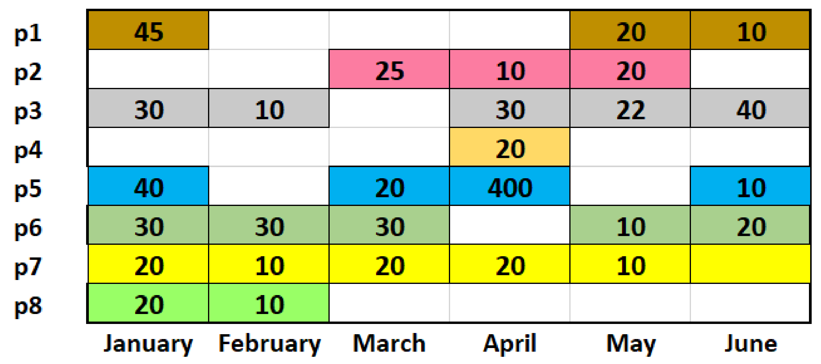
| Month | Products | |||||||
|---|---|---|---|---|---|---|---|---|
| P1 | P2 | P3 | P4 | P5 | P6 | P7 | P8 | |
| Initial stock | 1 | 0 | 1 | 1 | 1 | 1 | 0 | 0 |
| January | 45 | - | 30 | - | 40 | 30 | 20 | 20 |
| February | - | - | 10 | - | - | 30 | 10 | 10 |
| March | - | 25 | - | - | 20 | 30 | 20 | - |
| April | - | 10 | 30 | 20 | 400 | - | 20 | - |
| May | 20 | 20 | 22 | - | - | 10 | 10 | - |
| June | 10 | - | 40 | - | 10 | 20 | - | - |
| Resources | Products | |||||||
|---|---|---|---|---|---|---|---|---|
| P1 | P2 | P3 | P4 | P5 | P6 | P7 | P8 | |
| 4 | 5 | - | - | - | - | - | 5 | |
| - | 3 | 2 | 2 | 5 | - | - | - | |
| - | 2 | - | - | 7 | 7 | - | - | |
| - | - | - | - | - | 4 | 1 | 5 | |
| Production Resource | The Current Level of Use of R1..R4 |
|---|---|
| 30.67% | |
| 75.57% | |
| 8.25% | |
| 45.78% |
| Type of Warehouse | Maximum Capacity |
|---|---|
| 1000 square metres/height 5 m | |
| 100 square metres |
| Products | Volume |
|---|---|
| .. | 0.05 cubic meter |
| Meta-Model Elements | Symbol | Model Elements | Description |
|---|---|---|---|
| Sets & indexes | product | ||
| machine | |||
| time period , —initial period, —end period | |||
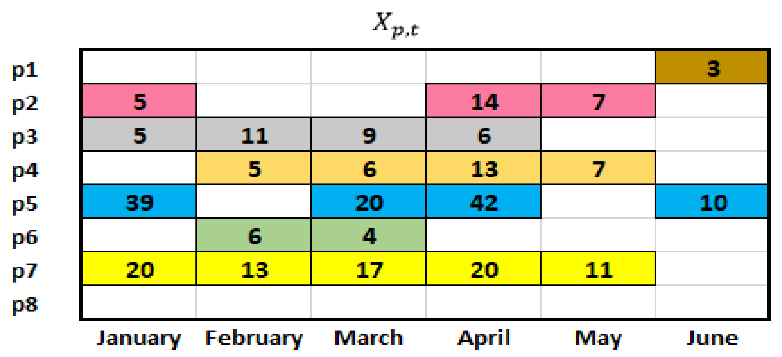
| Decision variables | production volume of the product in the period . | ||
| what order quantity for the product in period we are not able to fulfill | |||
| if the machine is not to be maintenance in period else . | |||
| if the overhaul of the machine cannot be performed, then else | |||
| Determined values | stock of product at the end of period | ||
| product storage cost | |||
| penalties for non-fulfillment of orders and maintenances | |||
| how many scheduled maintenances have not been carried out | |||
| how many products in total have not been comp. for all orders | |||
| Parameters | fulfilment of customer orders | ||
| ep | initial stock of the product | ||
| np | product storage volume | ||
| hp,r | factor determines how much time the product p must be processed on the machine . If hp,r1 ≠ 0 i hp,r2 ≠ 0 means that the product is made must be processed on a machine i . Value hp,r = 0 means product does not need to be processed on a machine r. | ||
| Any machine r in the period t has a specific production capacity (parameter value ) | |||
| Factor = 1 means that the maintenance of machines should be planned where means that such maintenance is not planned. | |||
| m_r | planned machine maintenance in the planning period | ||
| kp | kp—the maximum number of product p that may be in stock | ||
| v_m | The total volume of the warehouse v_m | ||
| fp | product unit p in the warehouse for a time unit is associated with the incurring cost |
| Costs Storage | ||||||||||||||||||||||
|---|---|---|---|---|---|---|---|---|---|---|---|---|---|---|---|---|---|---|---|---|---|---|
| t | 1 | 2 | 3 | 4 | 5 | 6 | t | 1 | 2 | 3 | 4 | 5 | 6 | 2000 | ||||||||
| p1 | 0 | 0 | 0 | 0 | 0 | 3 | p1 | 40 | 4 | 0 | 0 | 20 | 7 | |||||||||
| p2 | 5 | 0 | 0 | 14 | 7 | 0 | p2 | 0 | 0 | 20 | 0 | 9 | 0 | t | 1 | 2 | 3 | 4 | 5 | 6 | ||
| p3 | 5 | 11 | 9 | 6 | 0 | 0 | p3 | 24 | 0 | 3 | 17 | 22 | 40 | r1 | 0 | 1 | 1 | 1 | 1 | 1 | r1 0 | |
| p4 | 0 | 5 | 6 | 13 | 7 | 0 | p4 | 0 | 0 | 0 | 0 | 0 | 0 | r2 | 1 | 1 | 1 | 1 | 0 | 1 | r2 0 | |
| p5 | 39 | 0 | 20 | 42 | 0 | 10 | p5 | 0 | 0 | 0 | 358 | 0 | 0 | r3 | 1 | 1 | 1 | 1 | 1 | 1 | r3 1 | |
| p6 | 0 | 6 | 4 | 0 | 0 | 0 | p6 | 29 | 24 | 26 | 0 | 10 | 20 | r4 | 1 | 1 | 1 | 1 | 1 | 0 | r4 0 | |
| p7 | 20 | 13 | 17 | 20 | 11 | 0 | p7 | 0 | 0 | 0 | 0 | 9 | 0 | |||||||||
| p8 | 0 | 0 | 0 | 0 | 0 | 0 | p8 | 22 | 8 | 0 | 0 | 0 | 0 | |||||||||
| Share of Storage Costs in the Production Process | Classification Label |
|---|---|
| storage costs <50% | 1 |
| storage costs >50% and storage costs = 0 | 0 |
| Input Variables/Output Variables |
|---|
| —number of products |
| —planning horizon |
| —number of machines |
| —penalty for failure to perform maintenances |
| —penalty for failure to fulfil orders |
| —total storage capacity |
| —product storage volume |
| —initial stock of the product |
| —product storage cost p per time unit |
| —product storage cost p per time unit |
| —is there any planned overhaul of the machine? |
| —sales of P product in the period T |
| —machine production capacity R in the period T |
| —how much time does it take to process the product P on the machine R? |
| —assessment of storage costs according to the criterion |
Disclaimer/Publisher’s Note: The statements, opinions and data contained in all publications are solely those of the individual author(s) and contributor(s) and not of MDPI and/or the editor(s). MDPI and/or the editor(s) disclaim responsibility for any injury to people or property resulting from any ideas, methods, instructions or products referred to in the content. |
© 2023 by the authors. Licensee MDPI, Basel, Switzerland. This article is an open access article distributed under the terms and conditions of the Creative Commons Attribution (CC BY) license (https://creativecommons.org/licenses/by/4.0/).
Share and Cite
Juzoń, Z.; Wikarek, J.; Sitek, P. Application of Enterprise Architecture and Artificial Neural Networks to Optimize the Production Process. Electronics 2023, 12, 2015. https://doi.org/10.3390/electronics12092015
Juzoń Z, Wikarek J, Sitek P. Application of Enterprise Architecture and Artificial Neural Networks to Optimize the Production Process. Electronics. 2023; 12(9):2015. https://doi.org/10.3390/electronics12092015
Chicago/Turabian StyleJuzoń, Zbigniew, Jarosław Wikarek, and Paweł Sitek. 2023. "Application of Enterprise Architecture and Artificial Neural Networks to Optimize the Production Process" Electronics 12, no. 9: 2015. https://doi.org/10.3390/electronics12092015