
Image Inpainting with Parallel Decoding Structure for Future Internet
Abstract
:1. Introduction
2. Related Work
2.1. GAN
2.2. Attention Mechanism
3. Methodology
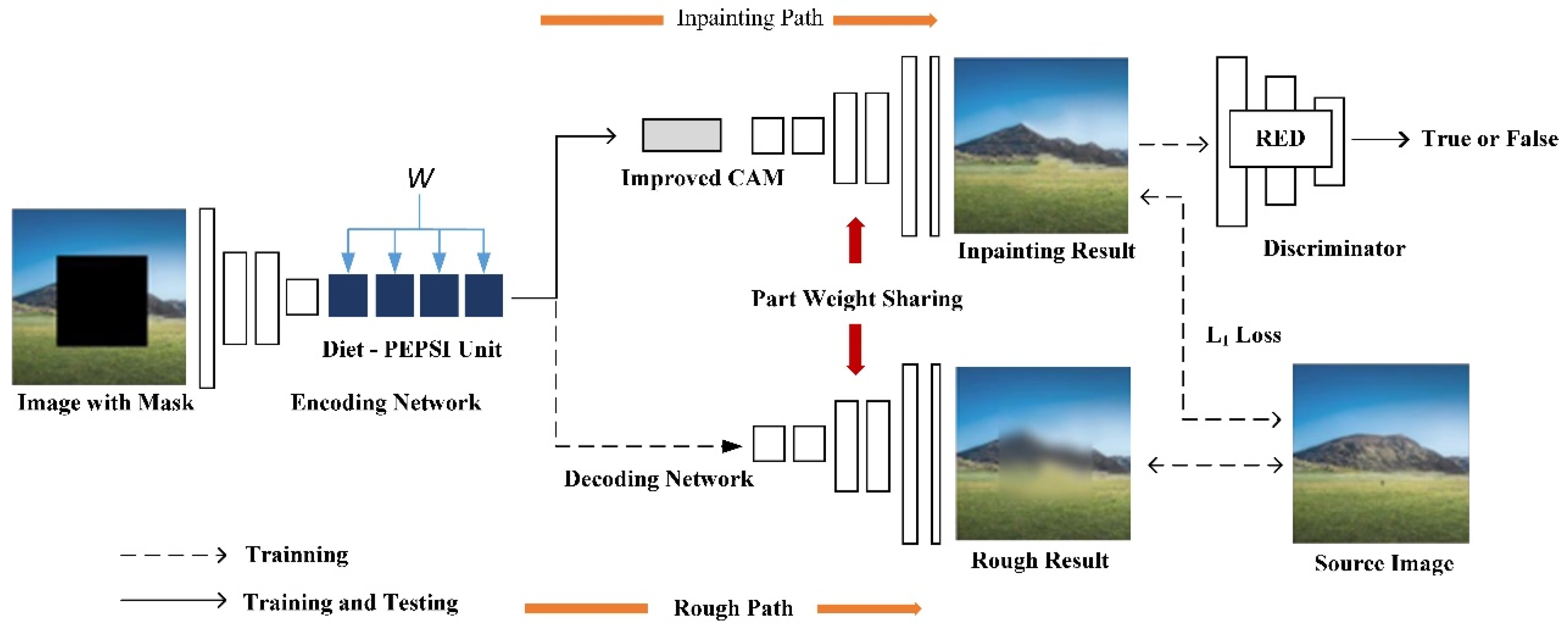
3.1. Model Frame
3.1.1. Network Model
3.1.2. Encoding Network
3.1.3. Decoding Network
3.2. Network Improvement
3.2.1. Diet-PEPSI Unit
3.2.2. Improved CAM
3.2.3. RED
3.3. Design of Loss Function
4. Experiments
4.1. Experimental Settings
4.2. Evaluation Metrics
4.3. Experimental Results and Analysis
4.3.1. Diet-PEPSI Unit Validation
4.3.2. Improved CAM Validation
4.3.3. RED Validation
4.3.4. Qualitative Assessments
4.3.5. Quantitative Assessments
5. Conclusions
Author Contributions
Funding
Acknowledgments
Conflicts of Interest
References
- Zhang, Y.; Zhao, P.; Ma, Y.; Fan, X. Multi-focus image fusion with joint guided image filtering. Signal Process. Image Commun. 2021, 92, 116–128. [Google Scholar] [CrossRef]
- Wang, N.; Zhang, Y.; Zhang, L. Dynamic selection network for image inpainting. IEEE Trans. Image Process. 2021, 30, 1784–1798. [Google Scholar] [CrossRef]
- Chen, Y.; Xia, R.; Zou, K.; Yang, K. FFTI: Image inpainting algorithm via features fusion and two-steps inpainting. J. Vis. Commun. Image Represent. 2023, 91, 103776. [Google Scholar] [CrossRef]
- Liu, K.; Li, J.; Hussain Bukhari, S.S. Overview of Image Inpainting and Forensic Technology. Secur. Commun. Netw. 2022, 2022, 9291971. [Google Scholar] [CrossRef]
- Phutke, S.; Murala, S. Image inpainting via spatial projections. Pattern Recognit. 2023, 133, 109040. [Google Scholar] [CrossRef]
- Zhang, L.; Zou, Y.; Yousuf, M.; Wang, W.; Jin, Z.; Su, Y.; Kim, S. BDSS: Blockchain-based Data Sharing Scheme with Fine-grained Access Control And Permission Revocation In Medical Environment. KSII Trans. Internet Inf. Syst. (TIIS) 2022, 16, 1634–1652. [Google Scholar]
- Huang, L.; Huang, Y. DRGAN: A dual resolution guided low-resolution image inpainting. Knowl.-Based Syst. 2023, 264, 110346. [Google Scholar] [CrossRef]
- Ran, C.; Li, X.; Yang, F. Multi-Step Structure Image Inpainting Model with Attention Mechanism. Sensors 2023, 23, 2316. [Google Scholar] [CrossRef]
- Li, A.; Zhao, L.; Zuo, Z.; Wang, Z.; Xing, W.; Lu, D. MIGT: Multi-modal image inpainting guided with text. Neurocomputing 2023, 520, 376–385. [Google Scholar] [CrossRef]
- Zhang, Y.; Ding, F.; Kwong, S.; Zhu, G. Feature pyramid network for diffusion-based image inpainting detection. Inf. Sci. 2021, 572, 29–42. [Google Scholar] [CrossRef]
- Zhang, Y.; Liu, T.; Cattani, C.; Cui, Q.; Liu, S. Diffusion-based image inpainting forensics via weighted least squares filtering enhancement. Multimed. Tools Appl. 2021, 80, 30725–30739. [Google Scholar] [CrossRef]
- Guo, Q.; Gao, S.; Zhang, X.; Yin, Y.; Zhang, C. Patch-based image inpainting via two-stage low rank approximation. IEEE Trans. Vis. Comput. Graph. 2017, 24, 2023–2036. [Google Scholar] [CrossRef]
- Newson, A.; Almansa, A.; Gousseau, Y.; Pérez, P. Non-local patch-based image inpainting. Image Process. Line 2017, 7, 373–385. [Google Scholar] [CrossRef]
- Tran, A.; Tran, H. Data-driven high-fidelity 2D microstructure reconstruction via non-local patch-based image inpainting. Acta Mater. 2019, 178, 207–218. [Google Scholar] [CrossRef]
- Kaur, G.; Sinha, R.; Tiwari, P.; Yadav, S.; Pandey, P.; Raj, R.; Rakhra, M. Face mask recognition system using CNN model. Neurosci. Inform. 2022, 2, 100035. [Google Scholar] [CrossRef]
- Liu, L.; Liu, Y. Load image inpainting: An improved U-Net based load missing data recovery method. Appl. Energy 2022, 327, 119988. [Google Scholar] [CrossRef]
- Zeng, Y.; Gong, Y.; Zhang, J. Feature learning and patch matching for diverse image inpainting. Pattern Recognit. 2021, 119, 108036. [Google Scholar] [CrossRef]
- Goodfellow, I.; Pouget-Abadie, J.; Mirza, M.; Xu, B.; Warde-Farley, D.; Ozair, S.; Bengio, Y. Generative adversarial networks. Commun. ACM 2020, 63, 139–144. [Google Scholar] [CrossRef]
- Pathak, D.; Krahenbuhl, P.; Donahue, J.; Darrell, T.; Efros, A. Context encoders: Feature learning by inpainting. In Proceedings of the IEEE Conference on Computer Vision and Pattern Recognition, Las Vegas, NV, USA, 27–30 June 2016; pp. 2536–2544. [Google Scholar]
- Yu, J.; Lin, Z.; Yang, J.; Shen, X.; Lu, X.; Huang, T. Generative image inpainting with contextual attention. In Proceedings of the IEEE Conference on Computer Vision and Pattern Recognition, Salt Lake City, UT, USA, 18–22 June 2018; pp. 5505–5514. [Google Scholar]
- Zhang, L.; Huang, T.; Hu, X.; Zhang, Z.; Wang, W.; Guan, D.; Kim, S. A distributed covert channel of the packet ordering enhancement model based on data compression. CMC-Comput. Mater. Contin. 2020, 64, 2013–2030. [Google Scholar]
- Zhang, L.; Wang, J.; Wang, W.; Jin, Z.; Zhao, C.; Cai, Z.; Chen, H. A novel smart contract vulnerability detection method based on information graph and ensemble learning. Sensors 2022, 22, 3581. [Google Scholar] [CrossRef]
- Zhang, L.; Wang, J.; Wang, W.; Jin, Z.; Su, Y.; Chen, H. Smart contract vulnerability detection combined with multi-objective detection. Comput. Netw. 2022, 217, 109289. [Google Scholar] [CrossRef]
- Qin, J.; Bai, H.; Zhao, Y. Multi-scale attention network for image inpainting. Comput. Vis. Image Underst. 2021, 204, 103155. [Google Scholar] [CrossRef]
- Shao, M.; Zhang, W.; Zuo, W.; Meng, D. Multi-scale generative adversarial inpainting network based on cross-layer attention transfer mechanism. Knowl.-Based Syst. 2020, 196, 105778. [Google Scholar] [CrossRef]
- Yan, Z.; Li, X.; Li, M.; Zuo, W.; Shan, S. Shift-net: Image inpainting via deep feature rearrangement. In Proceedings of the European Conference on Computer Vision (ECCV), Munich, Germany, 8–14 September 2018; pp. 1–17. [Google Scholar]
- Song, Y.; Yang, C.; Lin, Z.; Liu, X.; Huang, Q.; Li, H. Contextual-based image inpainting: Infer, match, and translate. In Proceedings of the European Conference on Computer Vision (ECCV), Munich, Germany, 8–14 September 2018; pp. 3–19. [Google Scholar]
- Sagong, M.; Shin, Y.; Kim, S. Pepsi: Fast image inpainting with parallel decoding network. In Proceedings of the IEEE/CVF Conference on Computer Vision and Pattern Recognition, Long Beach, CA, USA, 16–17 June 2019; pp. 11360–11368. [Google Scholar]
- Shin, Y.; Sagong, M.; Yeo, Y. Pepsi++: Fast and lightweight network for image inpainting. IEEE Trans. Neural Netw. Learn. Syst. 2020, 32, 252–265. [Google Scholar] [CrossRef] [Green Version]
- Wang, X.; Chen, Y.; Yamasaki, T. Spatially adaptive multi-scale contextual attention for image inpainting. Multimed. Tools Appl. 2022, 81, 31831–31846. [Google Scholar] [CrossRef]
- Ren, J.; Yu, C.; Ma, X. Balanced meta-softmax for long-tailed visual recognition. Adv. Neural Inf. Process. Syst. 2020, 33, 4175–4186. [Google Scholar]
- Bale, A.; Kumar, S.; Mohan, K. A Study of Improved Methods on Image Inpainting. In Trends and Advancements of Image Processing and Its Applications; Springer: Cham, Switzerland, 2022; pp. 281–296. [Google Scholar]
- Maniatopoulos, A.; Mitianoudis, N. Learnable Leaky ReLU (LeLeLU): An Alternative Accuracy-Optimized Activation Function. Information 2021, 12, 513. [Google Scholar] [CrossRef]
- Karras, T.; Aittala, M.; Laine, S. Alias-free generative adversarial networks. Adv. Neural Inf. Process. Syst. 2021, 34, 852–863. [Google Scholar]
- Yavuz, M.; Ahmed, S.; Kısaağa, M. YFCC-CelebA Face Attributes Datasets. In Proceedings of the 29th Signal Processing and Communications Applications Conference (SIU), Istanbul, Turkey, 9–11 June 2021; pp. 1–4. [Google Scholar]
- Karras, T.; Aila, T.; Laine, S.; Lehtinen, J. Progressive growing of GANs for improved quality, stability, and variation. In Proceedings of the International Conference on Learning Representations (ICLR), Vancouver, BC, Canada, 30 April–3 May 2018; pp. 1–26. [Google Scholar]
- Rezki, A.; Serir, A.; Beghdadi, A. Blind image inpainting quality assessment using local features continuity. Multimed. Tools Appl. 2022, 81, 9225–9244. [Google Scholar] [CrossRef]
- Ding, K.; Ma, K.; Wang, S.; Simoncelli, E. Image quality assessment: Unifying structure and texture similarity. IEEE Trans. Pattern Anal. Mach. Intell. 2020, 44, 2567–2581. [Google Scholar] [CrossRef]
- Zhang, W.; Ma, K.; Zhai, G.; Yang, X. Uncertainty-aware blind image quality assessment in the laboratory and wild. IEEE Trans. Image Process. 2021, 30, 3474–3486. [Google Scholar] [CrossRef] [PubMed]
- Yang, Y.; Cheng, Z.; Yu, H. MSE-Net: Generative image inpainting with multi-scale encoder. Vis. Comput. 2022, 38, 2647–2659. [Google Scholar] [CrossRef]
- Utama, K.; Umar, R.; Yudhana, A. Comparative Analysis of PSNR, Histogram and Contrast using Edge Detection Methods for Image Quality Optimization. J. Teknol. Dan Sist. Komput. 2022, 10, 67–71. [Google Scholar]
- Bakurov, I.; Buzzelli, M.; Schettini, R. Structural similarity index (SSIM) revisited: A data-driven approach. Expert Syst. Appl. 2022, 189, 116087. [Google Scholar] [CrossRef]


| Type | Kernel | Dilation | Stride | Outputs |
|---|---|---|---|---|
| Convolution | 5 × 5 | 1 | 1 × 1 | 32 |
| Convolution | 3 × 3 | 1 | 2 × 2 | 64 |
| Convolution | 3 × 3 | 1 | 1 × 1 | 64 |
| Convolution | 3 × 3 | 1 | 2 × 2 | 128 |
| Convolution | 3 × 3 | 1 | 1 × 1 | 128 |
| Convolution | 3 × 3 | 1 | 2 × 2 | 256 |
| Dilated Convolution | 3 × 3 | 2 | 1 × 1 | 256 |
| Dilated Convolution | 3 × 3 | 4 | 1 × 1 | 256 |
| Dilated Convolution | 3 × 3 | 8 | 1 × 1 | 256 |
| Dilated Convolution | 3 × 3 | 16 | 1 × 1 | 256 |
| Type | Kernel | Dilation | Stride | Outputs |
|---|---|---|---|---|
| Convolution × 2 | 3 × 3 | 1 | 1 × 1 | 128 |
| Upsample (×2↑) | - | - | - | - |
| Convolution × 2 | 3 × 3 | 1 | 1 × 1 | 64 |
| Upsample (×2↑) | - | - | - | - |
| Convolution × 2 | 3 × 3 | 1 | 1 × 1 | 32 |
| Upsample (×2↑) | - | - | - | - |
| Convolution × 2 | 3 × 3 | 1 | 1 × 1 | 16 |
| Convolution (output) | 3 × 3 | 1 | 1 × 1 | 3 |
| Type | Kernel | Stride | Outputs |
|---|---|---|---|
| Convolution | 5 × 5 | 2 × 2 | 64 |
| Convolution | 5 × 5 | 2 × 2 | 128 |
| Convolution | 5 × 5 | 2 × 2 | 256 |
| Convolution | 5 × 5 | 2 × 2 | 256 |
| Convolution | 5 × 5 | 2 × 2 | 256 |
| Convolution | 5 × 5 | 2 × 2 | 512 |
| FC | 1 × 1 | 1 × 1 | 1 |
| Net Model | PSNR/dB | SSIM/% | Time/ms | PQ/M |
|---|---|---|---|---|
| CE | 23.7 | 0.895 | 21.4 | 5.8 |
| GCA | 26.2 | 0.894 | 9.2 | 3.5 |
| PEPSI | 26.8 | 0.899 | 10.2 | 3.9 |
| Ours | 27.2 | 0.901 | 10.8 | 2.5 |
| Net Model | PSNR/dB | SSIM/% | Time/ms | PQ/M |
|---|---|---|---|---|
| CE | 22.8 | 0.899 | 22.5 | 5.8 |
| GCA | 24.1 | 0.912 | 9.4 | 3.5 |
| PEPSI | 28.5 | 0.925 | 11.1 | 3.9 |
| Ours | 28.7 | 0.928 | 11.9 | 2.5 |
Disclaimer/Publisher’s Note: The statements, opinions and data contained in all publications are solely those of the individual author(s) and contributor(s) and not of MDPI and/or the editor(s). MDPI and/or the editor(s) disclaim responsibility for any injury to people or property resulting from any ideas, methods, instructions or products referred to in the content. |
© 2023 by the authors. Licensee MDPI, Basel, Switzerland. This article is an open access article distributed under the terms and conditions of the Creative Commons Attribution (CC BY) license (https://creativecommons.org/licenses/by/4.0/).
Share and Cite
Zhao, P.; Chen, B.; Fan, X.; Chen, H.; Zhang, Y. Image Inpainting with Parallel Decoding Structure for Future Internet. Electronics 2023, 12, 1872. https://doi.org/10.3390/electronics12081872
Zhao P, Chen B, Fan X, Chen H, Zhang Y. Image Inpainting with Parallel Decoding Structure for Future Internet. Electronics. 2023; 12(8):1872. https://doi.org/10.3390/electronics12081872
Chicago/Turabian StyleZhao, Peng, Bowei Chen, Xunli Fan, Haipeng Chen, and Yongxin Zhang. 2023. "Image Inpainting with Parallel Decoding Structure for Future Internet" Electronics 12, no. 8: 1872. https://doi.org/10.3390/electronics12081872