Sum Rate Optimization for Multiple Access in Multi-FD-UAV-Assisted NOMA-Enabled Backscatter Communication Network

Abstract

With the rapid development of the Internet of Things (IoT) network, research on low-power and energy-saving devices has attracted extensive attention from both academia and the industry. Although the backscatter devices (BDs) that utilize the environmental power to activate circuits and transmit signals are a promising technology to be deployed as IoT nodes, it is challenging to design a flexible data backhaul scheme for massive BDs. Therefore, in this paper, we consider an unmanned-aerial-vehicle (UAV)-assisted backscatter communication network, where BDs are served by multiple full-duplex (FD) UAVs with the non-orthogonal multiple access (NOMA) schemes and modulate their signals on the downlink signals, which are generated by the UAVs to serve the coexisting regular user equipments (UEs). To maximize the sum rate of the considered system, we construct an optimization problem to optimize the reflection coefficient of BDs, the downlink and the backhaul transmission power, and the trajectory of UAVs jointly. Since the formulated problem is a non-convex optimization problem and is difficult to solve directly, we decouple the original problem into three sub-problems and solve them with the successive convex approximation (SCA) method, thereby addressing the original problem by a block coordinate descent (BCD)-based iterative algorithm. The simulation results show that, compared with the benchmark schemes, the proposed algorithm can obtain the highest system sum rate and utilize limited time-frequency resources more efficiently.

1. Introduction

As a typical scenario of the future wireless communication networks, the internet of things (IoT) is changing the way of future life with the emergence of new applications, such as power sensing, smart factories, and smart cities [1,2,3]. With the rapid development of the IoT industry, a massive scale of devices should be densely arranged in vast areas to fulfill the sensing requirements. Under the small size of the external structure, the energy storage and power supply of sensing devices are limited. To improve the device’s lifetime and save the cost of extensive device deployment, low-power communication transmission technologies have a broad vision of application and received widespread attention. As typical self-sustainable and low-power devices, backscatter devices (BDs) can transmit information by reflecting the existing environmental signals, which can be regarded as a promising solution to enable battery-free communications [4,5].

1.1. Overview and Motivation

In Ref. [6], the authors provide an overview of the fundamentals, applications and challenges of backscatter communications (BackCom). Ref. [7] provided a literature survey of the BackCom system and focused on the key signal processing techniques applied in this system. In existing works about BackCom, the authors in Refs. [8,9,10] developed theoretical analysis of the BackCom system to provide an accurate assessment of the system performance. Ref. [8] performed ergodic rate analysis and derived the upper bound of the backscatter link. Ref. [9] provided an outage performance analysis of BackComs. Ref. [10] conducted a coverage probability analysis by considering the interference of two communication links in the BackCom system. Then, the throughput and the energy efficiency of the system were both considered to be improved by optimizing the schedule strategy of BDs. In Refs. [11,12,13], the scheduling method of BDs was optimized to maximize the overall throughput of the BackCom system. In Ref. [14], a low-complexity method was proposed to jointly optimize the transmit power and the reflection coefficients of BDs. The authors in Ref. [15] considered the fairness between the BDs and optimized the resource allocation scheme to maximize the max–min throughput of the hybrid backscattering and harvest-then-transmit system. In particular, a deep reinforcement learning (DRL)-aided resource allocation method for both the BDs and UEs was investigated in Ref. [16] to improve the overall throughput of the system. In Ref. [17], a Gini threshold-based method was proposed to maximize the energy efficiency through balancing the traffic load of each BD. In Ref. [18], the authors considered the fairness of BDs and jointly optimized the transmission power and reflection coefficients to maximize the max–min energy efficiency of BDs. In addition, some of the literature investigated the code and decoding scheme of the BackCom system. Ref. [19] proposed an energy-efficient code scheme for the BackCom to minimize energy consumption. In Ref. [20], multiple readers were assumed to work cooperatively to collect the signals from BDs, and a joint receiving algorithm was designed to reduce the interference.

In the BackCom system, to assist the BDs in completing the signal transmission, the carrier emitters (CEs) and readers must be deployed to generate and receive the signals, respectively. Since BDs need a forward haul process under a passive method to transmit signals, the energy of the received signals at the reader side is usually low [7]. Therefore, in a wide region where BDs are distributed, there is also a vital requirement for dense deployment of CEs and readers to ensure successful data reception and decoding, which result in an unfordable burden to low-power IoT systems. To address this issue, integrating unmanned-aerial-vehicles (UAVs) with BackCom is an attractive technology that can reduce the cost of implementing the system [21]. With high flexibility and motility, the UAV can move close to the distributed BDs to efficiently complete energy supply or signal collection, making them well-suited for deployment as CEs or readers in the BackCom system.

In Ref. [22], the fixed CEs on the ground and a flying reader in UAV are considered to serve the BDs. In this paper, the trajectory of the UAV, the transmitting power of CE, and the orthogonal multiple access (OMA) scheduling of BDs are jointly optimized to improve the energy efficiency of the system. In Ref. [23], UAV acts as a relay to collect the data from BDs and upload them to the base station. The authors consider the energy constraint in the UAV and optimize its locations for data collection to maximize energy efficiency. In Ref. [24], UAV is treated as a flying BD to forward the signal to the base station. The trajectory of UAV, as well as the time-splitting method between the backscattering and common transmitting, are jointly optimized to maximize the throughput. In Refs. [25,26,27,28], the UAV was operated as both the CE and the reader. In Ref. [25], the authors consider the security problem and optimize the scheduling of BDs to maximize the secrecy rate. In Ref. [26], the UAV trajectory, resource allocation, and reflection coefficient of BDs are jointly optimized to maximize the ergodic capacity of the UAV-aided BackCom system. In Ref. [27], the mobility of UAV was explored to implement the over-the-air computation for the BackCom network, where the UAV flies over the coverage area obtain the sum channel gain from BDs in several samples and utilize the samples to assist the decoding of the signals transmitted by BDs. Ref. [28] proposed a deep reinforcement learning-based algorithm to design the trajectory of UAV to improve energy efficiency.

To further improve the efficiency of data acquisition and accelerate the aggregation of data from a large number of BDs in a short time, some of the literature investigated the integration of non-orthogonal multiple access (NOMA) with the BackCom. In Ref. [29], the grouping method and the adjusting strategy of each BD was solved to maximize the sum rate in a NOMA-aided BackCom system. In Ref. [30], the fairness between BDs was considered, and the scheduling method of BDs with the NOMA scheme was optimized to maximize the max–min throughput of the system. The authors in Ref. [31] considered the power constraint of both the BD and transmitter, then proposed a power allocation scheme to maximize the capacity of this system. In Ref. [32], the authors optimized the transmitting power and the reflection coefficient for NOMA-aided BackCom by taking into account the imperfect successive interference cancellation decoder to improve the sum rate. The work in Ref. [33] investigates the BackCom system under NOMA and full-duplex (FD) transmission, where the resource allocation scheme for the fixed base station is optimized to maximize the throughput of the common users and the BDs. In particular, the studies in Refs. [34,35,36] focus on merging UAV and NOMA jointly to assist backscatter communications. According to the operation and internal structure of the devices, we can classify the backscatter devices into three categories, that is, the monostatic backscatter, the bistatic backscatter, and the ambient backscatter [6,7]. In contrast to the other two BDs, the ambient backscatters modulate the signal on the available ambient sources to further reduce the cost of the BackCom system [37], which are mainly considered in this paper.

The analysis and optimization of the existing work have investigated the scenario where a single UAV is deployed to assist the BackCom. However, considering the wide distributed region and the limited energy supply capacity of BDs, a joint operation of multiple UAVs is essential for ensuring the performance of the BackCom system, which has not yet been researched as far as we know.

1.2. Paper Contribution

In this paper, we consider multiple full-duplex UAVs cooperate to serve the BDs with the NOMA scheme, while transmitting the downlink signal to normal users. We aim to provide an analytical framework for the multi-FD-UAV-assisted NOMA-enhanced backscatter communication system, and further consider the interference between the backscattering communication from the BDs and the active communication from the UEs. The main contributions of this paper are summarized as follows:

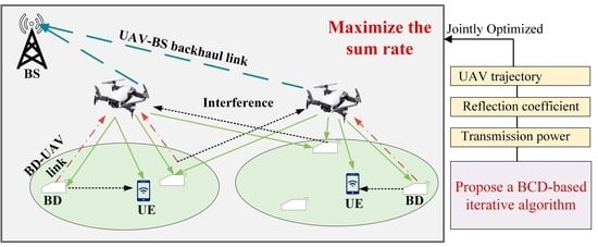
• We consider a multi-FD-UAV-assisted NOMA-enabled backscatter communication network, where multiple FD-UAVs are deployed to cooperate to serve the ground BDs with the NOMA scheme while communicating with the downlink UE. Then, the UAVs forward back the data of BDs to a nearby BS through the OMA scheme. To maximize the sum rate of BDs under the considered system, we formulate a sum rate maximization problem to jointly optimize the reflection coefficient of BDs, the downlink and the backhaul transmission power, and the trajectory of UAVs with constraints such as the successive interference cancellation (SIC) decoding constraints and the backhaul capacity constraint.
• Due to the non-convexity of the constructed problem, we split the original problem into three sub-problems, that is, the BD reflection coefficient optimization problem, the UAV transmission power optimization problem, and the UAV trajectory optimization problem. Then we apply the successive convex approximation (SCA) method to solve each sub-problem. Based on the solution of each sub-problem, we propose a block coordinate descent (BCD)-based iterative algorithm to solve the original problem. Furthermore, the convergence and complexity of the proposed algorithm are also proven.
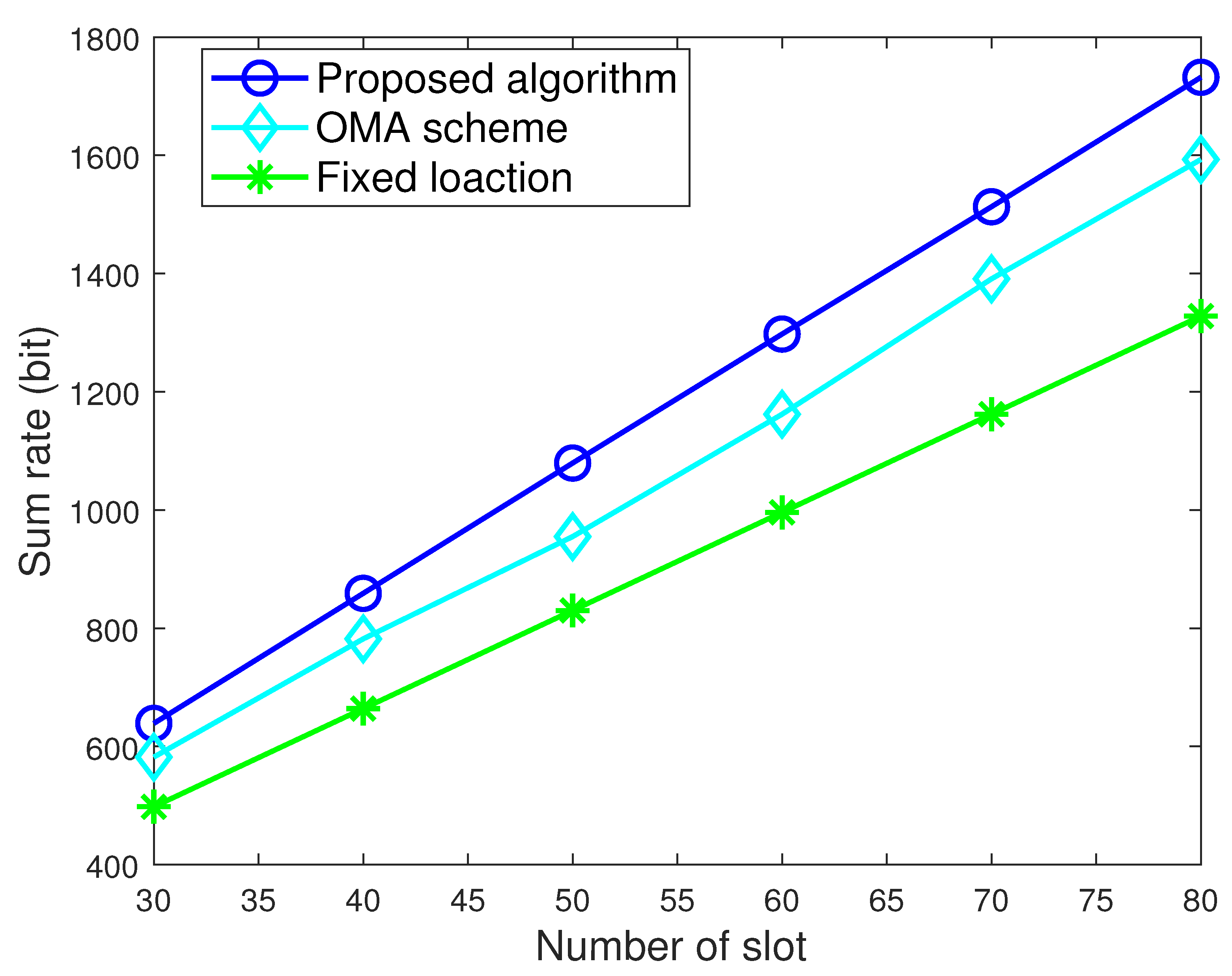
• To verify the effectiveness of the proposed algorithm, we provide extensive numerical results. The numerical results show that the proposed algorithm outperforms the two benchmark schemes, and the fast convergence of the proposed algorithm is also verified.

1.3. Paper Organization

The rest of the paper is organized as follows. Section 2 presents the system model of the multi-FD-UAV-assisted NOMA-enabled backscatter communication system and formulates the optimization problem. Section 3 provides the details about the proposed optimization algorithm. In Section 4, the numerical simulation results are presented. Then, Section 5 concludes this paper.

2. System Model

As shown in Figure 1, we consider a multi-FD-UAV-assisted NOMA-enabled backscatter communication network, where U flying rotary-wing UAVs are deployed to serve I downlink ground UEs at the fixed height. The index sets of UAVs and UEs are represented as $\mathcal{U}=\{1,2,\cdots ,U\}$ and $\mathcal{I}=\{1,2,\cdots ,I\}$. For convenience, we assume that each UE is fixed and only served by one UAV, that is, $U=I$. The BDs are randomly distributed in the service area of UAVs, and the BD index set is defined as $\mathcal{D}=\{1,2,\cdots ,D\}$. Each UAV is assumed to operate at the full duplex mode as [38,39]. To improve the communication efficiency and fully utilize the resources, as each UAV transmits downlink signals to the UEs, it simultaneously collects the signals reflected from BDs. Specifically, the BDs modulate their own signals to the signals sent by the UAVs towards the UEs [33,40]. Then, the UAVs decode the signals and forward them to the BS.

To illustrate the considered network clearly, we adopt the 3D Cartesian coordination to describe the positions of the UAVs, UEs, BDs, and BS. Let ${\mathit{S}}_u\left(t\right)=(x_u\left(t\right),y_u\left(t\right),h_{\mathrm{uav}})$, ${\mathit{S}}_i^{\mathrm{UE}}=(x_i,y_i,0)$, ${\mathit{B}}_d=(x_d,y_d,0)$ and $\mathit{W}=(x,y,h_{\mathrm{BS}})$ denote the coordinate of the u-th UAV, the i-th UE, the d-th BD and the BS at the time t for $\forall u\in \mathcal{U}$, $\forall i\in \mathcal{I}$ and $\forall d\in \mathcal{D}$, respectively. For analytical convenience, we denote T as the total service time of the UAVs, and we discretize it into Q slots, each with a duration as $\Delta t=T/Q$. Therefore, the trajectory of the UAVs can be further expressed as ${\mathit{S}}_u\left(q\right)=(x_u\left(q\right),y_u\left(q\right),h_{\mathrm{uav}})$ for $\forall q\in \{1,2,\cdots ,Q\}$. In the considered system, each UAV provides service for one UE and a set of BDs, namely a cell.

2.1. UAV-BD Link Transmission Model

In this work, the BDs access the UAV by reflecting the transmitted downlink signal with the power-domain NOMA scheme. For the associations between the BDs and UAVs, each BD can only associate with one UAV in one slot. Let ${\alpha }_{d,m}\left[q\right]$ denote the association indicator of BDs, which illustrates whether the d-th BD accesses the U-th UAV at the q-th slot. Specifically, the association indicator ${\alpha }_{d,m}\left[q\right]=1$ when the d-th BD accesses the u-th UAV; otherwise ${\alpha }_{d,m}\left[q\right]=0$.

Without loss of generality, we assume that information is shared between the UAVs (e.g., the UAV location information and UE data). Therefore, the UAV is able to eliminate the downlink UE signals sent by another UAV. Furthermore, the associated UAV can decode the data that the BD modulates on the transmitted signal of other UAVs. As a result, the received signal at the d-th BD is obtained as

$$\begin{array}{c}\hfill r_d^{\mathrm{BD}}\left[q\right]=\sum _{u=1}^U\sqrt{h_{u,d}^{\mathrm{u}-\mathrm{b}}\left[q\right]P_u\left[q\right]}{s}_u\left[q\right]+z_{\mathrm{d}}\left[q\right],\end{array}$$

(1)

where $P_u\left[q\right]$ and $s_u\left[q\right]$ represent the downlink transmission power and the u-th UAV data symbols at the q-th slot, respectively. $z_{\mathrm{d}}$ denotes the additive white Gaussian noise (AWGN) with zero mean and variance ${\sigma }_{\mathrm{d}}^2$ at the BD. In this work, all the channel links are assumed to be Rayleigh channels dependent on the path loss [41]. Considering the buildings or the trees would block the line-of-sight (LoS) path, our channel hypothesis combines the LoS and non-line-of-sight (NLoS) paths, that is, we assume that all channels in the same cell are the LoS channel similar to Refs. [22,39], while the channels between different cells will be dominated by NLoS path loss. Therefore, the channel from the u-th UAV to the d-th BD at the q-th slot $h_{u,d}^{\mathrm{u}-\mathrm{b}}\left[q\right]$ in (1) can be expressed as

$$\begin{array}{cc}\hfill & h_{u,d}^{\mathrm{u}-\mathrm{b}}\left[q\right]={\left(\frac{c}{4\pi d_{u,d}^{\mathrm{u}-\mathrm{b}}\left[q\right]f_{c1}\eta }\right)}^2,\hfill \end{array}$$

(2)

where $f_{c1}$ and c denote the carrier frequency for the UAV downlink and speed light in vacuum, respectively. The coefficients $\eta$ represent the additional attenuation. The distance from the u-th UAV to the d-th BD $d_{u,d}^{\mathrm{u}-\mathrm{b}}\left[q\right]$ is defined as $d_{u,d}^{\mathrm{u}-\mathrm{b}}\left[q\right]=\left|\right|{\mathit{S}}_u\left[q\right]-{\mathit{B}}_d\left|\right|$, where the operation $\left|\right|·\left|\right|$ denotes 2 norms.

Based on the received signals, the d-th BD activates the circuit and sends its own data $s_d$. Then the signal at the u-th UAV is given by

$$\begin{array}{cc}\hfill r_u^{\mathrm{UAV}}\left[q\right]& =\sum _{d=1}^D\sum _{u^{\prime }=1}^U{\alpha }_{d,u^{\prime }}\left[q\right]\sqrt{h_{u,d}^{\mathrm{u}-\mathrm{b}}\left[q\right]{\beta }_d\left[q\right]}{r}_d^{\mathrm{BD}}\left[q\right]s_d\left[q\right]+z_{\mathrm{u}}\left[q\right]\hfill \\ \hfill =& \sum _{d=1}^D\sum _{u^{\prime }=1}^U{\alpha }_{d,u^{\prime }}\left[q\right]\sqrt{h_{u,d}^{\mathrm{u}-\mathrm{b}}\left[q\right]{\beta }_d\left[q\right]}\sum _{j=1}^U\sqrt{h_{j,d}^{\mathrm{u}-\mathrm{b}}\left[q\right]P_j\left[q\right]}{s}_j\left[q\right]s_d\left[q\right]\hfill \\ \hfill & +\sum _{d=1}^D\sum _{u^{\prime }=1}^U{\alpha }_{d,u^{\prime }}\left[q\right]\sqrt{h_{u,d}^{\mathrm{u}-\mathrm{b}}\left[q\right]{\beta }_d\left[q\right]}{s}_d\left[q\right]z_{\mathrm{b}}+z_{\mathrm{u}}\left[q\right],\hfill \end{array}$$

(3)

where ${\beta }_d\left[q\right]$ denotes the reflection coefficient of the d-th BD and $z_{\mathrm{u}}$ is the zero mean AWGN noise with variance ${\sigma }_{\mathrm{u}}^2$ at the UAV. Since the BDs access the UAVs by the NOMA scheme, the UAVs adopt the SIC method to decode the data of the BDs. In order to obtain a better decoding result, the decoding order of the SIC is from UEs with better channels to those with poorer channel conditions. To clarify the decoding order, we define a channel strength comparison indicator as ${\lambda }_{i,j,u}\left[q\right]$ to demonstrate the strength relationship between two UAV-BD channels. Specifically, ${\lambda }_{i,j,u}\left[q\right]=0$ represents that the channel strength of the BD i is weaker than that of BD j when accessing the UAV u at slot q. Then the UAV first decodes the BD j data by considering the signal of BD i as interference. Otherwise, ${\lambda }_{i,j,u}\left[q\right]=1$.

Therefore, the signal-to-interference and noise ratio (SINR) of the BD d at the UAV u is given by

$$\begin{array}{c}\hfill {\gamma }_{d,u}\left[q\right]=\frac{{\alpha }_{d,u}\left[q\right]h_{u,d}^{\mathrm{u}-\mathrm{b}}\left[q\right]{\beta }_d\left[q\right]{\displaystyle \sum _{j=1}^U}{h}_{j,d}^{\mathrm{u}-\mathrm{b}}\left[q\right]P_j\left[q\right]}{{\displaystyle \sum _{d^{\prime }=1}^D}{\alpha }_{d^{\prime },u}\left[q\right]{\beta }_d\left[q\right]{\lambda }_{d,d^{\prime },u}\left[q\right]h_{u,d}^{\mathrm{u}-\mathrm{b}}\left[q\right]{\displaystyle \sum _{j=1}^U}{h}_{j,d^{\prime }}^{\mathrm{u}-\mathrm{b}}\left[q\right]P_j\left[q\right]+{\widehat{\mathcal{I}}}_u\left[q\right]+{\sigma }_{\mathrm{u}}^2},\end{array}$$

(4)

where ${\widehat{\mathcal{I}}}_u\left[q\right]$ is

$$\begin{array}{c}\hfill {\widehat{\mathcal{I}}}_u\left[q\right]={\displaystyle \sum _{d^{\prime }=1}^D}{\displaystyle \sum _{\begin{array}{c}m=1,\\ m\ne u\end{array}}^U}{\alpha }_{d^{\prime },m}\left[q\right]{\beta }_{d^{\prime }}\left[q\right]h_{u,d^{\prime }}^{\mathrm{u}-\mathrm{b}}\left[q\right]\sum _{j=1}^U{h}_{j,d^{\prime }}^{\mathrm{u}-\mathrm{b}}\left[q\right]P_j\left[q\right]+\sum _{d^{\prime }=1}^D\sum _{m=1}^U{\alpha }_{d^{\prime },m}\left[q\right]{\beta }_{d^{\prime }}\left[q\right]h_{u,d^{\prime }}^{\mathrm{u}-\mathrm{b}}\left[q\right]{\sigma }_{\mathrm{b}}^2.\end{array}$$

(5)

Generally, to ensure the successful decoding of the SIC method, the SINR of accessing BDs must be greater than a threshold, which can be denoted as

$${\gamma }_{d,u}\left[q\right]\ge \kappa ,$$

(6)

where $\kappa$ is defined as the given SINR threshold.

Then the sum rate at the UAV u can be obtained as

$$\begin{array}{c}\hfill R_u\left[q\right]=\sum _{d=1}^D{\alpha }_{i,u}log(1+{\gamma }_{d,u}\left[q\right]).\end{array}$$

(7)

Specifically, according to Ref. [42], we can simplify $R_u\left[q\right]$ as

$$\begin{array}{cc}\hfill R_u\left[q\right]& ={\displaystyle \sum _{d=1}^D}log\left(1+\frac{{\alpha }_{d,u}\left[q\right]h_{u,d}^{\mathrm{u}-\mathrm{b}}\left[q\right]{\beta }_d\left[q\right]{\displaystyle \sum _{j=1}^U}{h}_{j,d}^{\mathrm{u}-\mathrm{b}}\left[q\right]P_j\left[q\right]}{{\displaystyle \sum _{d^{\prime }=1}^D}{\alpha }_{d^{\prime },u}\left[q\right]{\beta }_d\left[q\right]{\lambda }_{d,d^{\prime },u}\left[q\right]h_{u,d}^{\mathrm{u}-\mathrm{b}}\left[q\right]{\displaystyle \sum _{j=1}^U}{h}_{j,d^{\prime }}^{\mathrm{u}-\mathrm{b}}\left[q\right]P_j\left[q\right]+{\widehat{\mathcal{I}}}_u\left[q\right]+{\sigma }_{\mathrm{u}}^2}\right)\hfill \\ \hfill & =log\left(1+\frac{{\displaystyle \sum _{d^{\prime }=1}^D}{\alpha }_{d^{\prime },u}\left[q\right]{\beta }_{d^{\prime }}\left[q\right]h_{u,d^{\prime }}^{\mathrm{u}-\mathrm{b}}\left[q\right]{\displaystyle \sum _{j=1}^U}{h}_{j,d^{\prime }}^{\mathrm{u}-\mathrm{b}}\left[q\right]P_j\left[q\right]}{{\widehat{\mathcal{I}}}_u\left[q\right]+{\sigma }_{\mathrm{u}}^2}\right).\hfill \end{array}$$

(8)

2.2. UAV-UE Link Transmission Model

For the ground UEs, since each UE is allowed to connect one UAV, we denote ${\theta }_{u,i}\left[q\right]$ as the association indicator to describe the service state between the i-th UE and the u-th UAV at the q-th slot. The association indicator ${\theta }_{u,i}\left[q\right]=1$ when the i-th UE is served by u-th UAV; otherwise, ${\theta }_{u,i}\left[q\right]=0$. Therefore, the signal received at the i-th UE is given by

$$\begin{array}{c}\hfill r_i\left[q\right]={\displaystyle \sum _{u=1}^U}\sqrt{h_{u,i}^{\mathrm{u}-\mathrm{u}}\left[q\right]P_u\left[q\right]}{s}_u\left[q\right]+{\displaystyle \sum _{d=1}^D}{\displaystyle \sum _{u=1}^U}{\alpha }_{d,u}\left[q\right]r_d^{\mathrm{BD}}\left[q\right]s_d\left[q\right]+z_{\mathrm{ue},i}\left[q\right],\end{array}$$

(9)

where $P_u\left[q\right]$ and $s_u\left[q\right]$ represent the downlink transmission power and the data symbols of the u-th UAV at the q-th slot, respectively, and $h_{u,i}^{\mathrm{u}-\mathrm{u}}\left[q\right]$ is denoted as the average channel gain from the u-th UAV to the i-th UE at the q-th slot, that is,

$$\begin{array}{cc}\hfill & h_{u,i}^{\mathrm{u}-\mathrm{u}}\left[q\right]={\left(\frac{c}{4\pi d_{u,i}^{\mathrm{u}-\mathrm{u}}\left[q\right]f_{c1}\eta }\right)}^2,\hfill \end{array}$$

(10)

where $d_{u,i}^{\mathrm{u}-\mathrm{u}}\left[q\right]=\left|\right|{\mathit{S}}_u\left[q\right]-{\mathit{S}}_i^{\mathrm{UE}}\left|\right|$.

The second term on the right side of (9) is the interference of BD to the UE, and $z_{\mathrm{ue},i}$ denotes the additive AWGN at the UE with zero mean and variance ${\sigma }_{\mathrm{ue}}^2$. Therefore, the sum rate for the i-th UE is obtained as

$$\begin{array}{cc}\hfill & R_i^{\mathrm{u}}\left[q\right]=\hfill \\ \hfill & log\left(1+\frac{{\displaystyle \sum _{u=1}^U}{\theta }_{u,i}\left[q\right]h_{u,i}^{\mathrm{u}-\mathrm{u}}\left[q\right]P_u\left[q\right]}{{\displaystyle \sum _{u=1}^U}{\displaystyle \sum _{\begin{array}{c}{i}^{\prime }=1,\\ i^{\prime }\ne i\end{array}}^I}{\theta }_{u,i^{\prime }}\left[q\right]h_{u,i^{\prime }}^{\mathrm{u}-\mathrm{u}}\left[q\right]P_u\left[q\right]+{\displaystyle \sum _{d=1}^D}{\displaystyle {\displaystyle \sum _{u=1}^U}}{\alpha }_{d,u}\left[q\right]{\beta }_d\left[q\right]h_{d,i}^{\mathrm{b}-\mathrm{u}}({\displaystyle \sum _{m=1}^U}{h}_{u,d}^{\mathrm{u}-\mathrm{b}}\left[q\right]P_u\left[q\right]+{\sigma }_{\mathrm{b}}^2)+{\sigma }_{\mathrm{ue}}^2}\right),\hfill \end{array}$$

(11)

where $h_{d,i}^{\mathrm{b}-\mathrm{u}}$ is the average channel gain from the b-th BD to the i-th UE, which can be expressed as

$$\begin{array}{c}\hfill h_{d,i}^{\mathrm{b}-\mathrm{u}}={\left(\frac{c}{4\pi d_{d,i}^{\mathrm{b}-\mathrm{u}}{f}_{c1}\eta }\right)}^2,\end{array}$$

(12)

where $d_{d,i}^{\mathrm{b}-\mathrm{u}}=\left|\right|{\mathit{B}}_d-{\mathit{S}}_i^{\mathrm{UE}}\left|\right|$ is the distance from the d-th BD to the i-th UE.

2.3. UAV-BS Link Transmission Model

After decoding the signal from BDs, the UAVs will send them to the adjacent BS through the backhaul link. Due to the small number of UAVs, the backhaul link of UAV-BS is transmitted with the OMA scheme to enhance the backhaul capacity. Let $P_u^B\left[q\right]$ denote the transmission power of the UAV u at the slot q in the backhaul link. The sum rate at the BS for the UAV u can be obtained as

$$\begin{array}{c}\hfill R_u^B\left[q\right]=log(1+\frac{P_u^B\left[q\right]h_u^{\mathrm{u}-\mathrm{B}}\left[q\right]}{{\sigma }_{\mathrm{B}}^2}),\end{array}$$

(13)

where ${\sigma }_{\mathrm{B}}^2$ is a variance of the AWGN noise at the BS and $h_u^{\mathrm{u}-\mathrm{B}}$ is the average channel gain from the u-th UAV to the BS, that is,

$$\begin{array}{c}\hfill h_u^{\mathrm{u}-\mathrm{B}}\left[q\right]={\left(\frac{c}{4\pi d_u^{\mathrm{u}-\mathrm{B}}\left[q\right]f_{c2}\eta }\right)}^2,\end{array}$$

(14)

where $f_{c2}$ denotes the carrier frequency for the UAV-BS backhaul link and $d_u^{\mathrm{u}-\mathrm{B}}\left[q\right]$ is the distance from the U-th UAV to the BS, that is, $d_u^{\mathrm{u}-\mathrm{B}}\left[q\right]=\left|\right|{\mathit{S}}_u\left[q\right]-\mathit{W}\left|\right|$.

2.4. Problem Formulation

In this work, we aim to maximize the sum rate of the BDs by jointly optimizing the transmission power of UAVs, the reflection coefficient of BDs, and the trajectory of UAVs with the NOMA scheme. Let $\mathbf{\beta }\triangleq \{{\beta }_d\left[q\right],d\in \mathcal{D},q\in \mathcal{Q}\}$, $\mathit{P}\triangleq \{P_d\left[q\right],d\in \mathcal{D},q\in \mathcal{Q}\}$, and ${\mathit{P}}^{\mathrm{B}}\triangleq \{P_d^B\left[q\right],d\in \mathcal{D},q\in \mathcal{Q}\}$ denote the reflection coefficient of BDs, the downlink transmission power of UAVs and the backhaul transmission power of UAVs, respectively. Therefore, the sum rate optimization with the considered multi-FD-UAV-assisted NOMA-enabled backscatter communication network over Q slots is formulated as

$$\begin{array}{cc}\hfill \left(\mathbf{P}\mathbf{1}\right)& \underset{\mathit{S},\mathit{P},{\mathit{P}}^{\mathrm{B}},\mathbf{\beta }}{max}\sum _{q=1}^Q\sum _{u=1}^U{R}_u\left[q\right]\hfill \end{array}$$

(15)

$$\begin{array}{cc}& \mathrm{s}.\mathrm{t}.\left(6\right),\hfill \end{array}$$

(16)

$$\begin{array}{c}\hfill \sum _{q=1}^Q{R}_u^B\ge \sum _{q=1}^Q{R}_u\left[q\right],\forall u,\end{array}$$

(17)

$$\begin{array}{c}\hfill \sum _{q=1}^Q{R}_i^{\mathrm{u}}\left[q\right]\ge R_{\min }^{\mathrm{UE}},\forall i,\end{array}$$

(18)

$$\begin{array}{c}\hfill 0\le {\beta }_d\left[q\right]\le 1,\forall d,q,\end{array}$$

(19)

$$\begin{array}{c}\hfill \left|\right|{\mathit{S}}_u[q+1]-{\mathit{S}}_u\left[q\right]|{|}^2\le {(V_{max}\Delta t)}^2,\end{array}$$

(20)

$$\begin{array}{c}\hfill {\mathit{S}}_u\left[1\right]={\mathit{S}}_u\left[Q\right],\forall u,\end{array}$$

(21)

$$\begin{array}{c}\hfill \left|\right|{\mathit{S}}_u\left[q\right]-{\mathit{S}}_j\left[q\right]|{|}^2\ge d_{min}^2,\forall u,j,q,u\ne j,\end{array}$$

(22)

$$\begin{array}{c}\hfill 0\le P_d\left[q\right]\le P_{max},\forall d,q,\end{array}$$

(23)

$$\begin{array}{c}\hfill 0\le P_d^B\left[q\right]\le P_{max},\forall d,q,\end{array}$$

(24)

$$\begin{array}{c}\hfill 0\le P_d^B\left[q\right]+P_d\left[q\right]\le P_{max},\forall d,q,\end{array}$$

(25)

where the constraint (17) is to ensure that the capacity of the backhaul link is greater than the data transmitted by the BDs to prevent data from accumulating and overflowing at the UAVs. To satisfy the quality of service (QoS) of the UE, we have the minimum sum rate constraint for UEs as shown in (18), where $R_{\min }^{\mathrm{UE}}$ denote the minimum sum rate for each UE over all the slots. The reflection coefficient limitation of BDs is shown in (19). The inequalities (20) and (21) represent the speed constraint and the trajectory constraint, where $V_{max}$ is the maximum flying velocity. Given the minimum distance between two UAVs $d_{min}$, the inequality (22) ensures that collisions between UAVs do not occur. The inequality (23)–(25) are the power limitation of the UAVs, where $P_{max}$ represents the maximum transmission power of the UAV.

3. Proposed Algorithm for Sum Rate Maximization

Since the formulated Problem (P1) is intractable to solve due to the non-convexity of the objective function and the constraints, in this section, we propose a BCD-based iterative algorithm to jointly optimize the reflection coefficient, transmission power, and trajectory of the UAV. Specifically, we split Problem (P1) into three independent sub-problems, that is, the reflection coefficient optimization problem, the transmission power of the UAV problem, and the trajectory optimization problem. Then, we use the SCA method to convert each sub-problem into a convex problem and solve it. Furthermore, the complexity and the convergence of the proposed algorithm are given in this section.

3.1. Reflection Coefficients Optimization

Given the transmission power and the trajectory of the UAV, the reflection coefficients optimization problem can be obtained as

$$\begin{array}{cc}\hfill \left(\mathbf{P}\mathbf{2}\right)& \underset{\mathbf{\beta }}{max}\sum _{q=1}^Q\sum _{u=1}^U{R}_u\left[q\right]\hfill \end{array}$$

(26)

$$\begin{array}{cc}& \mathrm{s}.\mathrm{t}.\left(6\right),\left(7\right),\left(18\right),\left(19\right).\hfill \end{array}$$

(27)

However, the formulated Problem (P2) is still non-convex due to the fractional forms in the logarithm function. Therefore, we will simplify the logarithmic form and adopt the SCA method to solve the problem.

For the non-convexity of $R_u\left[q\right]$, based on (8), we first split it into $R_u\left[q\right]={\tilde{R}}_u\left[q\right]-{\widehat{R}}_u\left[q\right]$, where ${\tilde{R}}_u\left[q\right]$ and ${\widehat{R}}_u\left[q\right]$ are denoted as

$$\begin{array}{cc}\hfill {\tilde{R}}_u\left[q\right]& =log\left(\sum _{d=1}^D\sum _{m=1}^U{\alpha }_{d,m}\left[q\right]{\beta }_d\left[q\right]h_{u,d}^{\mathrm{u}-\mathrm{b}}\left[q\right]\sum _{j=1}^U{h}_{j,d}^{\mathrm{u}-\mathrm{b}}\left[q\right]P_j\left[q\right]+\sum _{d=1}^D\sum _{m=1}^U{\alpha }_{d,m}\left[q\right]{\beta }_d\left[q\right]h_{u,d}^{\mathrm{u}-\mathrm{b}}\left[q\right]{\sigma }_{\mathrm{b}}^2+{\sigma }_{\mathrm{u}}^2\right),\hfill \end{array}$$

(28)

$$\begin{array}{cc}\hfill {\widehat{R}}_u\left[q\right]& =log\left(\sum _{d=1}^D\sum _{\begin{array}{c}m=1,\\ m\ne u\end{array}}^U{\alpha }_{d,m}\left[q\right]{\beta }_d\left[q\right]h_{u,d}^{\mathrm{u}-\mathrm{b}}\left[q\right]\sum _{j=1}^U{h}_{j,d}^{\mathrm{u}-\mathrm{b}}\left[q\right]P_j\left[q\right]+\sum _{d=1}^D\sum _{m=1}^U{\alpha }_{d,m}\left[q\right]{\beta }_d\left[q\right]h_{u,d}^{\mathrm{u}-\mathrm{b}}\left[q\right]{\sigma }_{\mathrm{b}}^2+{\sigma }_{\mathrm{u}}^2\right),\hfill \end{array}$$

(29)

which are both concave with respect to (w.r.t.) ${\beta }_d\left[q\right]$. Therefore, to transform ${\widehat{R}}_u\left[q\right]$ to a convex function, we apply the first-order Taylor expansion (FTE) to ${\widehat{R}}_u\left[q\right]$ and we can obtain its upper bound as

$$\begin{array}{cc}\hfill {\widehat{R}}_u\left[q\right]\le & {\displaystyle \sum _{k=1}^D}\frac{{\displaystyle \sum _{m=1,m\ne u}^U}{\alpha }_{k,m}\left[q\right]h_{u,k}^{\mathrm{u}-\mathrm{b}}\left[q\right]{\displaystyle \sum _{j=1}^U}{h}_{j,k}^{\mathrm{u}-\mathrm{b}}\left[q\right]P_j\left[q\right]+{\displaystyle \sum _{m=1}^U}{\alpha }_{k,m}\left[q\right]h_{u,k}^{\mathrm{u}-\mathrm{b}}\left[q\right]{\sigma }_{\mathrm{u}}^2}{A_u^r\left[q\right]ln2}({\beta }_k\left[q\right]-{\beta }_k^r\left[q\right])\hfill \\ \hfill & +log\left(A_u^r\left[q\right]\right)\hfill \\ \hfill =& {{\widehat{R}}_u}^{\mathrm{up}}\left[q\right],\hfill \end{array}$$

(30)

where ${\beta }_k^r\left[q\right]$ is the local point at the r-th SCA iteration and $A_u^r\left[q\right]$ is denoted as

$$\begin{array}{c}\hfill A_u^r\left[q\right]={\displaystyle \sum _{d=1}^D}{\displaystyle \sum _{\begin{array}{c}m=1,\\ m\ne u\end{array}}^U}{\alpha }_{d,m}\left[q\right]{\beta }_d^r\left[q\right]h_{u,d}^{\mathrm{u}-\mathrm{b}}\left[q\right]{\displaystyle \sum _{j=1}^U}{h}_{j,d}^{\mathrm{u}-\mathrm{b}}\left[q\right]P_j\left[q\right]+{\displaystyle \sum _{d=1}^D}{\displaystyle \sum _{m=1}^U}{\alpha }_{d,m}\left[q\right]{\beta }_d^r\left[q\right]h_{u,d}^{\mathrm{u}-\mathrm{b}}\left[q\right]{\sigma }_{\mathrm{u}}^2+{\sigma }_{\mathrm{u}}^2.\end{array}$$

(31)

Therefore, the non-convexity of the objective function $R_u\left[q\right]$ is addressed. For the backhaul capacity constraint (17), since $R_u^B$ is convex w.r.t. ${\beta }_d\left[q\right]$, we need to transform $R_u\left[q\right]$ to a convex function. Therefore, based on (30), we can obtain the lower bound of ${\tilde{R}}_u\left[q\right]$ at the r-th iteration as

$$\begin{array}{cc}\hfill {\widehat{R}}_u\left[q\right]\ge & {\displaystyle \sum _{k=1}^K}\frac{{\displaystyle \sum _{m=1}^U}{\alpha }_{k,m}\left[q\right]h_{u,k}^{\mathrm{u}-\mathrm{b}}\left[q\right]{\displaystyle \sum _{j=1}^U}{h}_{j,k}^{\mathrm{u}-\mathrm{b}}\left[q\right]P_j\left[q\right]+{\displaystyle \sum _{m=1}^U}{\alpha }_{k,m}\left[q\right]h_{u,k}^{\mathrm{u}-\mathrm{b}}\left[q\right]{\sigma }_{\mathrm{u}}^2}{B_u^r\left[q\right]ln2}({\beta }_k\left[q\right]-{\beta }_k^r\left[q\right])\hfill \\ \hfill & +log\left(B_u^r\left[q\right]\right)\hfill \\ \hfill =& {{\widehat{R}}_u}^{\mathrm{lb}}\left[q\right],\hfill \end{array}$$

(32)

where $B_u^r\left[q\right]$ is denoted as

$$\begin{array}{c}\hfill B_u^r\left[q\right]={\displaystyle \sum _{d=1}^D}{\displaystyle \sum _{\begin{array}{c}m=1\end{array}}^U}{\alpha }_{d,m}\left[q\right]{\beta }_d^r\left[q\right]h_{u,d}^{\mathrm{u}-\mathrm{b}}\left[q\right]{\displaystyle \sum _{j=1}^U}{h}_{j,d}^{\mathrm{u}-\mathrm{b}}\left[q\right]P_j\left[q\right]+{\displaystyle \sum _{d=1}^D}{\displaystyle \sum _{m=1}^U}{\alpha }_{d,m}\left[q\right]{\beta }_d^r\left[q\right]h_{u,d}^{\mathrm{u}-\mathrm{b}}\left[q\right]{\sigma }_{\mathrm{b}}^2+{\sigma }_{\mathrm{u}}^2.\end{array}$$

(33)

Therefore, the constraint (17) is converted to be convex as

$$\begin{array}{c}\hfill \sum _{q=1}^Q{R}_u^B\ge \sum _{q=1}^Q{{\widehat{R}}_u}^{\mathrm{lb}}\left[q\right]+{\widehat{R}}_u\left[q\right],\forall u.\end{array}$$

(34)

For the constraint of QoS of the UE, following the similar steps of the transformation of the objective function $R_u\left[q\right]$, we can divide $R_i^{\mathrm{u}}\left[q\right]$ into two parts as $R_i^{\mathrm{u}}\left[q\right]={\tilde{R}}_i^{\mathrm{u}}\left[q\right]-{\widehat{R}}_i^{\mathrm{u}}\left[q\right]$, which can be specifically expressed as

$$\begin{array}{cc}\hfill & {\tilde{R}}_i^{\mathrm{u}}\left[q\right]\hfill \\ \hfill & =log\left(\sum _{u=1}^U\sum _{i^{\prime }=1}^I{\theta }_{u,i^{\prime }}\left[q\right]h_{u,i^{\prime }}^{\mathrm{u}-\mathrm{u}}\left[q\right]P_u\left[q\right]+\sum _{d=1}^D\sum _{m=1}^U{\alpha }_{d,m}\left[q\right]{\beta }_d\left[q\right]h_{d,i}^{\mathrm{b}-\mathrm{u}}(\sum _{u=1}^U{h}_{u,d}^{\mathrm{u}-\mathrm{b}}\left[q\right]P_u\left[q\right]+{\sigma }_{\mathrm{b}}^2)+{\sigma }_{\mathrm{u}}^2\right),\hfill \\ \hfill & {\widehat{R}}_i^{\mathrm{u}}\left[q\right]\hfill \end{array}$$

(35)

$$\begin{array}{cc}\hfill & =log\left({\displaystyle \sum _{u=1}^U}{\displaystyle \sum _{i^{\prime }=1,i^{\prime }\ne i}^I}{\theta }_{u,i^{\prime }}\left[q\right]h_{u,i^{\prime }}^{\mathrm{u}-\mathrm{u}}\left[q\right]P_u\left[q\right]+{\displaystyle \sum _{d=1}^D}{\displaystyle \sum _{m=1}^U}{\alpha }_{d,u}\left[q\right]{\beta }_d\left[q\right]h_{d,i}^{\mathrm{b}-\mathrm{u}}({\displaystyle \sum _{u=1}^U}{h}_{u,d}^{\mathrm{u}-\mathrm{b}}\left[q\right]P_u\left[q\right]+{\sigma }_{\mathrm{b}}^2)+{\sigma }_{\mathrm{u}}^2\right).\hfill \end{array}$$

(36)

Similarly, according to FTE, ${\widehat{R}}_i^{\mathrm{u}}\left[q\right]$ is upper-bounded by

$$\begin{array}{c}\hfill {\widehat{R}}_i^{\mathrm{u}}\left[q\right]\le log{C}_i^r\left[q\right]+{\displaystyle \sum _{k=1}^D}\frac{{\displaystyle \sum _{u=1}^U}{\alpha }_{k,u}\left[q\right]{\beta }_k^r\left[q\right]h_{k,i}^{\mathrm{b}-\mathrm{u}}({\displaystyle \sum _{m=1}^U}{h}_{u,k}^{\mathrm{u}-\mathrm{b}}\left[q\right]P_u\left[q\right]+{\sigma }_{\mathrm{b}}^2)}{C_i^r\left[q\right]ln2}({\beta }_k\left[q\right]-{\beta }_k^r\left[q\right])={\widehat{R}}_i^{\mathrm{u},\mathrm{up}}\left[q\right],\end{array}$$

(37)

where $C_i^r\left[q\right]$ is given by

$$\begin{array}{cc}\hfill & C_i^r\left[q\right]={\displaystyle \sum _{u=1}^U}{\displaystyle \sum _{\begin{array}{c}{i}^{\prime }=1,\\ i^{\prime }\ne i\end{array}}^I}{\theta }_{u,i^{\prime }}\left[q\right]h_{u,i^{\prime }}^{\mathrm{u}-\mathrm{u}}\left[q\right]P_u\left[q\right]+{\displaystyle \sum _{d=1}^D}{\displaystyle \sum _{u=1}^U}{\alpha }_{d,u}\left[q\right]{\beta }_d^r\left[q\right]h_{d,i}^{\mathrm{b}-\mathrm{u}}({\displaystyle \sum _{m=1}^U}{h}_{u,d}^{\mathrm{u}-\mathrm{b}}\left[q\right]P_u\left[q\right]+{\sigma }_{\mathrm{b}}^2)+{\sigma }_{\mathrm{u}}^2.\hfill \end{array}$$

(38)

Therefore, the constraint (18) is converted to be convex as

$$\begin{array}{c}\hfill \sum _{q=1}^Q{\tilde{R}}_i^{\mathrm{u}}\left[q\right]-{\widehat{R}}_i^{\mathrm{u},\mathrm{up}}\left[q\right]\ge R_{\min }^{\mathrm{UE}},\forall i.\end{array}$$

(39)

As for the SINR constraint (6), we can make it convex by the simple algebraic operation, which is expressed as

$$\begin{array}{cc}\hfill & \sum _{d=1}^D\sum _{m=1}^U{\alpha }_{d,m}\left[q\right]{\beta }_d\left[q\right]h_{u,d}^{\mathrm{u}-\mathrm{b}}\left[q\right]\sum _{j=1}^U{h}_{j,d}^{\mathrm{u}-\mathrm{b}}\left[q\right]P_j\left[q\right]\hfill \\ \hfill & \ge \kappa (\sum _{d=1}^D\sum _{\begin{array}{c}m=1,\\ m\ne u\end{array}}^U{\alpha }_{d,m}\left[q\right]{\beta }_d\left[q\right]h_{u,d}^{\mathrm{u}-\mathrm{b}}\left[q\right]\sum _{j=1}^U{h}_{j,d}^{\mathrm{u}-\mathrm{b}}\left[q\right]P_j\left[q\right]+\sum _{d=1}^D\sum _{m=1}^U{\alpha }_{d,m}\left[q\right]{\beta }_d\left[q\right]h_{u,d}^{\mathrm{u}-\mathrm{b}}\left[q\right]{\sigma }_{\mathrm{u}}^2+{\sigma }_{\mathrm{u}}^2).\hfill \end{array}$$

(40)

Consequently, with the SCA method, we can recast Problem (P2) at the r-th iteration as

$$\begin{array}{cc}\hfill \left(\mathbf{P}\mathbf{2}.\mathbf{1}\right)& \underset{\mathbf{\beta }}{max}\sum _{q=1}^Q\sum _{u=1}^U{\tilde{R}}_u\left[q\right]-{{\widehat{R}}_u}^{\mathrm{up}}\left[q\right]\hfill \end{array}$$

(41)

$$\begin{array}{cc}& \mathrm{s}.\mathrm{t}.\left(34\right),\left(34\right),\left(39\right),\left(40\right).\hfill \end{array}$$

(42)

Since Problem (P2.1) is convex w.r.t. the reflection coefficient $\mathbf{\beta }$, it can be solved directly by the standard convex tools.

3.2. UAV Transmission Power Optimization

With the given reflection coefficients of the BD $\mathbf{\beta }$ and the trajectory of the UAV $\mathit{S}$, the optimization problem w.r.t. the transmission power of UAV can be formulated as

$$\begin{array}{cc}\hfill \left(\mathbf{P}\mathbf{3}.\mathbf{1}\right)& \underset{\mathit{P},{\mathit{P}}^{\mathrm{B}}}{max}\sum _{q=1}^Q\sum _{u=1}^U{R}_u\left[q\right]\hfill \end{array}$$

(43)

$$\begin{array}{cc}& \mathrm{s}.\mathrm{t}.\left(6\right),\left(17\right),\left(18\right),\left(23\right),\left(24\right),\left(25\right).\hfill \end{array}$$

(44)

For the above Problem (3.1), we can find the constraints (23), (24), and (25) are jointly convex w.r.t. $\mathit{P}$ and ${\mathit{P}}^{\mathrm{B}}$. As for the constraint (6), we can rewrite it as

$$\begin{array}{cc}\hfill & {\alpha }_{d,m}\left[q\right]{\beta }_d\left[q\right]h_{u,d}^{\mathrm{u}-\mathrm{b}}\left[q\right]{\displaystyle \sum _{j=1}^U}{h}_{j,d}^{\mathrm{u}-\mathrm{b}}\left[q\right]P_j\left[q\right]\ge \kappa ({\displaystyle \sum _{d^{\prime }=1}^D}{\alpha }_{d^{\prime },u}\left[q\right]{\beta }_{d^{\prime }}\left[q\right]{\lambda }_{d,d^{\prime },u}\left[q\right]h_{u,d^{\prime }}^{\mathrm{u}-\mathrm{b}}\left[q\right]{\displaystyle \sum _{j=1}^U}{h}_{j,d^{\prime }}^{\mathrm{u}-\mathrm{b}}\left[q\right]P_j\left[q\right]+\hfill \\ \hfill & {\displaystyle \sum _{d^{\prime }=1}^D}{\displaystyle \sum _{\begin{array}{c}m=1,\\ m\ne u\end{array}}^U}{\alpha }_{d^{\prime },m}\left[q\right]{\beta }_{d^{\prime }}\left[q\right]h_{u,d^{\prime }}^{\mathrm{u}-\mathrm{b}}\left[q\right]{\displaystyle \sum _{j=1}^U}{h}_{j,d^{\prime }}^{\mathrm{u}-\mathrm{b}}\left[q\right]P_j\left[q\right]+{\displaystyle \sum _{d^{\prime }=1}^D}{\displaystyle \sum _{m=1}^U}{\alpha }_{d^{\prime },m}\left[q\right]{\beta }_d\left[q\right]h_{u,d^{\prime }}^{\mathrm{u}-\mathrm{b}}\left[q\right]{\sigma }_{\mathrm{b}}^2+{\sigma }_{\mathrm{u}}^2),\hfill \end{array}$$

(45)

which is convex w.r.t. $\mathit{P}$. As for the rest of the non-convex constraints, since Problem (3.1) w.r.t. the transmission power of UAV $\mathit{P}$ and ${\mathit{P}}^{\mathrm{B}}$ has the same structure as Problem (P2) w.r.t. the reflection coefficients $\mathbf{\beta }$, we can use the same transformation steps to convert Problem (3.1) into a convex problem.

Therefore, we can first obtain the convex lower bound of $R_u\left[q\right]$ as $R_u^{\mathrm{lb}}\left[q\right]={\tilde{R}}_u\left[q\right]-{{\widehat{R}}_u}^{\mathrm{up}}\left[q\right]$, where ${{\widehat{R}}_u}^{\mathrm{up}}\left[q\right]$ is obtained by applying FTE to ${\widehat{R}}_u\left[q\right]$ with the given point $P_u^r\left[r\right]$ at the r-th SCA iteration, which can be expressed as

$$\begin{array}{c}\hfill {{\widehat{R}}_u}^{\mathrm{up}}\left[q\right]=log{E}_u^r\left[q\right]+{\displaystyle \sum _{j^{\prime }=1}^U}\frac{{\displaystyle \sum _{d=1}^D}{\displaystyle \sum _{m=1,m\ne u}^U}{\alpha }_{d,m}\left[q\right]{\beta }_d^r\left[q\right]h_{u,d}^{\mathrm{u}-\mathrm{b}}{h}_{j^{\prime },d}^{\mathrm{u}-\mathrm{b}}\left[q\right]}{E_u^r\left[q\right]ln2}(P_{j^{\prime }}\left[q\right]-P_{j^{\prime }}^r\left[q\right]),\end{array}$$

(46)

where $E_u^r\left[q\right]$ is given by

$$\begin{array}{c}\hfill E_u^r\left[q\right]={\displaystyle \sum _{d=1}^D}{\displaystyle \sum _{\begin{array}{c}m=1,\\ m\ne u\end{array}}^U}{\alpha }_{d,m}\left[q\right]{\beta }_d\left[q\right]h_{u,d}^{\mathrm{u}-\mathrm{b}}\left[q\right]{\displaystyle \sum _{j=1}^U}{h}_{j,d}^{\mathrm{u}-\mathrm{b}}\left[q\right]P_j^r\left[q\right]+{\displaystyle \sum _{d=1}^D}{\displaystyle \sum _{m=1}^U}{\alpha }_{d,m}\left[q\right]{\beta }_d\left[q\right]h_{u,d}^{\mathrm{u}-\mathrm{b}}\left[q\right]{\sigma }_{\mathrm{b}}^2+{\sigma }_{\mathrm{u}}^2.\end{array}$$

(47)

For the backhaul capacity constraint (17) and UE QoS constraint (18), by using the same method as optimizing $\mathbf{\beta }$, we can obtain the transformed convex constraint as

$$\begin{array}{cc}\hfill & {\displaystyle \sum _{q=1}^Q}log\left(1+\frac{P_u^{\mathrm{B}}\left[q\right]h_u^{\mathrm{u}-\mathrm{B}}}{{\sigma }_{\mathrm{B}}^2}\right)\ge {\displaystyle \sum _{j^{\prime }=1}^U}\frac{{\displaystyle \sum _{d=1}^D}{\displaystyle \sum _{m=1}^U}{\alpha }_{d,m}\left[q\right]{\beta }_d^r\left[q\right]h_{u,d}^{\mathrm{u}-\mathrm{b}}{h}_{j^{\prime },d}^{\mathrm{u}-\mathrm{b}}\left[q\right]}{F_u^r\left[q\right]ln2}(P_{j^{\prime }}\left[q\right]-P_{j^{\prime }}^r\left[q\right])\hfill \end{array}$$

$$\begin{array}{cc}\hfill & -{\widehat{R}}_i^{\mathrm{u}}\left[q\right]+log{F}_u^r\left[q\right],\hfill \\ \hfill & {\displaystyle \sum _{q=1}^Q}{\tilde{R}}_i^{\mathrm{u}}\left[q\right]-log{G}_i^r\left[q\right]-{\displaystyle \sum _{j^{\prime }=1}^U}\frac{{\displaystyle \sum _{i^{\prime }=1,i^{\prime }\ne i}^U}{\theta }_{j^{\prime },i^{\prime }}{h}_{j^{\prime },i}^{\mathrm{u}-\mathrm{u}}\left[q\right]+{\sum }_d^D{\sum }_{u=1}^U{\alpha }_{d,u}\left[q\right]{\beta }_d\left[q\right]h_{d,i}^{\mathrm{b}-\mathrm{u}}{h}_{j^{\prime },d}^{\mathrm{u}-\mathrm{b}}\left[q\right]}{G_i^r\left[q\right]ln2}(P_{j^{\prime }}\left[q\right]-P_{j^{\prime }}^r\left[q\right])\hfill \end{array}$$

(48)

$$\begin{array}{cc}\hfill & \ge R_{\min }^{\mathrm{UE}},\hfill \end{array}$$

(49)

where $F_u^r\left[q\right]$ and $G_i^r\left[q\right]$ are given by

$$\begin{array}{cc}\hfill F_u^r\left[q\right]& ={\displaystyle \sum _{u=1}^U}{\displaystyle \sum _{i^{\prime }=1}^I}{\theta }_{u,i^{\prime }}\left[q\right]h_{u,i^{\prime }}^{\mathrm{u}-\mathrm{u}}\left[q\right]P_u^r\left[q\right]+{\displaystyle \sum _{d=1}^D}{\displaystyle \sum _{m=1}^U}{\alpha }_{d,m}\left[q\right]{\beta }_d\left[q\right]h_{d,i}^{\mathrm{b}-\mathrm{u}}({\displaystyle \sum _{u=1}^U}{h}_{u,d}^{\mathrm{u}-\mathrm{b}}\left[q\right]P_u^r\left[q\right]+{\sigma }_{\mathrm{b}}^2)+{\sigma }_{\mathrm{u}}^2,\hfill \end{array}$$

(50)

$$\begin{array}{cc}\hfill G_i^r\left[q\right]& ={\displaystyle \sum _{u=1}^U}{\displaystyle \sum _{i^{\prime }=1,i^{\prime }\ne i}^I}{\theta }_{u,i^{\prime }}\left[q\right]h_{u,i^{\prime }}^{\mathrm{u}-\mathrm{u}}\left[q\right]P_u\left[q\right]+{\displaystyle \sum _{d=1}^D}{\displaystyle \sum _{m=1}^U}{\alpha }_{d,u}\left[q\right]{\beta }_d\left[q\right]h_{d,i}^{\mathrm{b}-\mathrm{u}}({\displaystyle \sum _{u=1}^U}{h}_{u,d}^{\mathrm{u}-\mathrm{b}}\left[q\right]P_u\left[q\right]+{\sigma }_{\mathrm{b}}^2)+{\sigma }_{\mathrm{u}}^2.\hfill \end{array}$$

(51)

Therefore, the transmission power optimization problem can be reformulated as

$$\begin{array}{cc}\hfill \left(\mathbf{P}\mathbf{3}.\mathbf{2}\right)& \underset{\mathit{P},{\mathit{P}}^{\mathrm{B}}}{max}{\displaystyle \sum _{q=1}^Q}{\displaystyle \sum _{u=1}^U}{R}_u^{\mathrm{lb}}\left[q\right]\hfill \end{array}$$

(52)

$$\begin{array}{cc}& \mathrm{s}.\mathrm{t}.\left(23\right),\left(24\right),\left(25\right),\left(45\right),\left(48\right),\left(49\right).\hfill \end{array}$$

(53)

Since Problem (3.2) is a convex problem w.r.t. $\mathit{P}$ and ${\mathit{P}}^{\mathrm{B}}$, the standard convex tool can be applied directly to solve it.

3.3. Trajectory Optimization

Given the reflection coefficients of the BD $\mathbf{\beta }$ and the transmission power of the UAV $\mathit{P}$ and ${\mathit{P}}^{\mathrm{B}}$, the sum rate optimization problem w.r.t. the UAV trajectory can be recasted as

$$\begin{array}{cc}\hfill \left(\mathbf{P}\mathbf{4}.\mathbf{1}\right)& \underset{\mathit{S}}{max}{\displaystyle \sum _{q=1}^Q}{\displaystyle \sum _{u=1}^U}{R}_u\left[q\right]\hfill \end{array}$$

(54)

$$\begin{array}{cc}& \mathrm{s}.\mathrm{t}.\left(6\right),\left(17\right),\left(18\right),\left(20\right),\left(21\right),\left(22\right).\hfill \end{array}$$

(55)

Note that due to the non-convexity of the objective function and constraints, Problem (3.1) is neither concave nor convex; thus, we will adopt the SAC technique to solve it.

According to the channel definition (2) and the split of the sum rate of UAV $R_u\left[q\right]$, we can re-express ${\tilde{R}}_u\left[q\right]$ and ${\widehat{R}}_u\left[q\right]$ w.r.t. the trajectory of UAV $\mathit{S}$ as

$$\begin{array}{cc}\hfill {\tilde{R}}_u\left[q\right]& =log\left({\displaystyle \sum _{d=1}^D}{\displaystyle \sum _{m=1}^U}{\displaystyle \sum _{j=1}^U}\frac{{\alpha }_{d,m}\left[q\right]{\beta }_d\left[q\right]}{\left|\right|{\mathit{S}}_u\left[q\right]-{\mathit{B}}_d{\left|\right|}^2}\frac{{\mu }^2{P}_j\left[q\right]}{\left|\right|{\mathit{S}}_j\left[q\right]-{\mathit{B}}_d{\left|\right|}^2}+{\displaystyle \sum _{d=1}^D}{\displaystyle \sum _{m=1}^U}\frac{{\alpha }_{d,u}\left[q\right]{\beta }_d\left[q\right]\mu {\sigma }_{\mathrm{u}}^2}{\left|\right|{\mathit{S}}_u\left[q\right]-{\mathit{B}}_d{\left|\right|}^2}+{\sigma }_{\mathrm{u}}^2\right),\hfill \end{array}$$

(56)

$$\begin{array}{cc}\hfill {\widehat{R}}_u\left[q\right]& =log\left({\displaystyle \sum _{d=1}^D}{\displaystyle \sum _{m=1,m\ne u}^U}{\displaystyle \sum _{j=1}^U}\frac{{\alpha }_{d,m}\left[q\right]{\beta }_d\left[q\right]}{\left|\right|{\mathit{S}}_u\left[q\right]-{\mathit{B}}_d{\left|\right|}^2}\frac{{\mu }^2{P}_j\left[q\right]}{\left|\right|{\mathit{S}}_j\left[q\right]-{\mathit{B}}_d{\left|\right|}^2}+{\displaystyle \sum _{d=1}^D}{\displaystyle \sum _{m=1}^U}\frac{{\alpha }_{d,u}\left[q\right]{\beta }_d\left[q\right]\mu {\sigma }_{\mathrm{u}}^2}{\left|\right|{\mathit{S}}_u\left[q\right]-{\mathit{B}}_d{\left|\right|}^2}+{\sigma }_{\mathrm{u}}^2\right),\hfill \end{array}$$

(57)

where $\mu ={\left(\frac{c}{4\pi f_{c2}\eta }\right)}^2.$

According to Ref. [43], ${\tilde{R}}_u\left[q\right]$ and ${\widehat{R}}_u\left[q\right]$ are both convex w.r.t. $\left|\right|{\mathit{S}}_j\left[q\right]-{\mathit{B}}_d\left|\right|$ for $\forall j\in \mathcal{U}$, $d\in \mathcal{D}$. Therefore, we introduce the slack variable $\omega =\{{\omega }_{u,d}\left[q\right],\forall j\in \mathcal{U},d\in \mathcal{D},q\in \mathcal{Q}\}$ to ${\widehat{R}}_u\left[q\right]$ as

$$\begin{array}{cc}\hfill {\widehat{R}}_u\left[q\right]& \le log\left({\displaystyle \sum _{d=1}^D}{\displaystyle \sum _{m=1,m\ne u}^U}{\displaystyle \sum _{j=1}^U}\frac{{\alpha }_{d,m}\left[q\right]{\beta }_d\left[q\right]}{{\omega }_{u,d}\left[q\right]}\frac{{\mu }^2{P}_j\left[q\right]}{{\omega }_{j,d}\left[q\right]}+\sum _{d=1}^D\sum _{m=1}^U\frac{{\alpha }_{d,u}\left[q\right]{\beta }_d\left[q\right]\mu {\sigma }_{\mathrm{u}}^2}{{\omega }_{u,d}\left[q\right]}+{\sigma }_{\mathrm{u}}^2\right)\hfill \\ \hfill & ={{\widehat{R}}_u}^{\mathrm{up}}\left[q\right],\hfill \end{array}$$

(58)

with the following constraint as

$$\begin{array}{c}\hfill {\omega }_{u,d}\left[q\right]\le \left|\right|{\mathit{S}}_u\left[q\right]-{\mathit{B}}_d{\left|\right|}^2,\forall j\in \mathcal{U},d\in \mathcal{D},q\in \mathcal{Q}.\end{array}$$

(59)

Therefore, ${{\widehat{R}}_u}^{\mathrm{up}}\left[q\right]$ is a convex function but the constraint (59) is non-convex due to the convexity of $\left|\right|{\mathit{S}}_u\left[q\right]-{\mathit{B}}_d\left|\right|$. As a result, by applying FTE to $\left|\right|{\mathit{S}}_u\left[q\right]-{\mathit{B}}_d\left|\right|$ with the given point ${\mathit{S}}_u^r\left[q\right]$ at the r-th SCA iteration, the constraint (59) can be transformed into

$$\begin{array}{c}\hfill {\omega }_{u,d}\left[q\right]\le \left|\right|{\mathit{S}}_u^r\left[q\right]-{\mathit{B}}_d{\left|\right|}^2+2{({\mathit{S}}_u^r\left[q\right]-{\mathit{B}}_d)}^T({\mathit{S}}_u^r-{\mathit{B}}_d),\forall j\in \mathcal{U},d\in \mathcal{D},q\in \mathcal{Q},\end{array}$$

(60)

which is convex w.r.t. $\mathit{S}$.

For the convexity of ${\tilde{R}}_u\left[q\right]$, we apply the FTE to obtain the lower bound of ${\tilde{R}}_u\left[q\right]$ as

$$\begin{array}{cc}\hfill {\tilde{R}}_u\left[q\right]\ge & log\left(H_u^r\left[q\right]\right)+{\displaystyle \sum _{k=1}^D}\frac{{\displaystyle \sum _{m=1}^U}{\displaystyle \sum _{j=1}^U}\frac{{\alpha }_{k,m}\left[q\right]{\beta }_k\left[q\right]}{\left|\right|{\mathit{S}}_j^r\left[q\right]-{\mathit{B}}_k{\left|\right|}^2}\frac{-{\mu }^2{P}_j\left[q\right]}{\left|\right|{\mathit{S}}_u^r\left[q\right]-{\mathit{B}}_k{\left|\right|}^4}+{\displaystyle \sum _{m=1}^U}\frac{-{\alpha }_{k,u}\left[q\right]{\beta }_k\left[q\right]\mu {\sigma }_{\mathrm{u}}^2}{\left|\right|{\mathit{S}}_u\left[q\right]-{\mathit{B}}_k{\left|\right|}^4}}{H_u^r\left[q\right]ln2}\left(\right||{\mathit{S}}_u\left[q\right]-{\mathit{B}}_k{\left|\right|}^2\hfill \\ \hfill & -\left|\right|{\mathit{S}}_u^r\left[q\right]-{\mathit{B}}_k{\left|\right|}^2)+{\displaystyle \sum _{u^{\prime }=1}^U}{\displaystyle \sum _{k=1}^D}\frac{{\displaystyle \sum _{m=1}^U}\frac{{\alpha }_{k,m}\left[q\right]{\beta }_k\left[q\right]}{\left|\right|{\mathit{S}}_u^r\left[q\right]-{\mathit{B}}_k{\left|\right|}^2}\frac{-{\mu }^2{P}_{u^{\prime }}\left[q\right]}{\left|\right|{\mathit{S}}_{u^{\prime }}^r\left[q\right]-{\mathit{B}}_k{\left|\right|}^4}}{H_u^r\left[q\right]ln2}\left(\right||{\mathit{S}}_{u^{\prime }}\left[q\right]-{\mathit{B}}_k{\left|\right|}^2\hfill \\ \hfill & -\left|\right|{\mathit{S}}_{u^{\prime }}^r\left[q\right]-{\mathit{B}}_k{\left|\right|}^2)={{\tilde{R}}_u}^{\mathrm{lb}}\left[q\right],\hfill \end{array}$$

(61)

where $H_u^r\left[q\right]$ is denoted as

$$\begin{array}{c}\hfill H_u^r\left[q\right]={\displaystyle \sum _{d=1}^D}{\displaystyle \sum _{m=1}^U}{\displaystyle \sum _{j=1}^U}\frac{{\alpha }_{d,m}\left[q\right]{\beta }_d\left[q\right]}{\left|\right|{\mathit{S}}_u^r\left[q\right]-{\mathit{B}}_d\left|\right|}\frac{{\mu }^2{P}_j\left[q\right]}{\left|\right|{\mathit{S}}_j^r\left[q\right]-{\mathit{B}}_d\left|\right|}+{\displaystyle \sum _{d=1}^D}{\displaystyle \sum _{m=1}^U}\frac{{\alpha }_{d,u}\left[q\right]{\beta }_d\left[q\right]\mu {\sigma }_{\mathrm{u}}^2}{\left|\right|{\mathit{S}}_u^r\left[q\right]-{\mathit{B}}_d\left|\right|}+{\sigma }_{\mathrm{u}}^2.\end{array}$$

(62)

Therefore, we obtain the lower bound on the sum rate $R_u^{\mathrm{lb}}\left[q\right]={{\tilde{R}}_u}^{\mathrm{lb}}\left[q\right]-{{\widehat{R}}_u}^{\mathrm{up}}\left[q\right]$, which is concave w.r.t. $\mathit{S}$.

For the backhaul capacity constraint (17), we need to convert $R_u\left[q\right]$ to a convex function. Therefore, by using the FTE to ${\widehat{R}}_u\left[q\right]$, ${\widehat{R}}_u\left[q\right]$ can be lower bounded by

$$\begin{array}{cc}\hfill {\widehat{R}}_u\left[q\right]\ge & log\left(J_u^r\left[q\right]\right)+{\displaystyle \sum _{k=1}^D}\frac{{\displaystyle \sum _{\begin{array}{c}m=1,\\ m\ne u\end{array}}^U}{\displaystyle \sum _{j=1}^U}\frac{{\alpha }_{k,m}\left[q\right]{\beta }_k\left[q\right]}{\left|\right|{\mathit{S}}_j^r\left[q\right]-{\mathit{B}}_k{\left|\right|}^2}\frac{-{\mu }^2{P}_j\left[q\right]}{\left|\right|{\mathit{S}}_u^r\left[q\right]-{\mathit{B}}_k{\left|\right|}^4}+{\displaystyle \sum _{m=1}^U}\frac{-{\alpha }_{k,u}\left[q\right]{\beta }_k\left[q\right]\mu {\sigma }_{\mathrm{u}}^2}{\left|\right|{\mathit{S}}_u\left[q\right]-{\mathit{B}}_k{\left|\right|}^4}}{J_u^r\left[q\right]ln2}\left(\right||{\mathit{S}}_u\left[q\right]-{\mathit{B}}_k{\left|\right|}^2\hfill \\ \hfill & -\left|\right|{\mathit{S}}_u^r\left[q\right]-{\mathit{B}}_k{\left|\right|}^2)+{\displaystyle \sum _{u^{\prime }=1}^U}{\displaystyle \sum _{k=1}^D}\frac{{\displaystyle \sum _{m=1,m\ne u}^U}\frac{{\alpha }_{k,m}\left[q\right]{\beta }_k\left[q\right]}{\left|\right|{\mathbf{Q}}_u^r\left[q\right]-{\mathit{B}}_k{\left|\right|}^2}\frac{-{\mu }^2{P}_{u^{\prime }}\left[q\right]}{\left|\right|{\mathit{S}}_{u^{\prime }}^r\left[q\right]-{\mathit{B}}_k{\left|\right|}^4}}{J_u^r\left[q\right]ln2}\left(\right||{\mathit{S}}_{u^{\prime }}\left[q\right]-{\mathit{B}}_k{\left|\right|}^2\hfill \\ \hfill & -\left|\right|{\mathit{S}}_{u^{\prime }}^r\left[q\right]-{\mathit{B}}_k{\left|\right|}^2)={{\widehat{R}}_u}^{\mathrm{lb}}\left[q\right],\hfill \end{array}$$

(63)

where $J_u^r\left[q\right]$ is denoted as

$$\begin{array}{c}\hfill J_u^r\left[q\right]=\sum _{d=1}^D\sum _{m=1,m\ne u}^U\sum _{j=1}^U\frac{{\alpha }_{d,m}\left[q\right]{\beta }_d\left[q\right]}{\left|\right|{\mathit{S}}_u^r\left[q\right]-{\mathit{B}}_d\left|\right|}\frac{{\mu }^2{P}_j\left[q\right]}{\left|\right|{\mathit{S}}_j^r\left[q\right]-{\mathit{B}}_d\left|\right|}+\sum _{d=1}^D\sum _{m=1}^U\frac{{\alpha }_{d,u}\left[q\right]{\beta }_d\left[q\right]\mu {\sigma }_{\mathrm{u}}^2}{\left|\right|{\mathit{S}}_u^r\left[q\right]-{\mathit{B}}_d\left|\right|}+{\sigma }_{\mathrm{u}}^2.\end{array}$$

(64)

Meanwhile, with the slack variable $\omega$, we can obtain the upper bound of ${\tilde{R}}_u\left[q\right]$ as

$$\begin{array}{cc}\hfill {\tilde{R}}_u\left[q\right]& \le log\left(\sum _{d=1}^D\sum _{m=1}^U\sum _{j=1}^U\frac{{\alpha }_{d,m}\left[q\right]{\beta }_d\left[q\right]}{{\omega }_{u,d}\left[q\right]}\frac{{\mu }^2{P}_j\left[q\right]}{{\omega }_{j,d}\left[q\right]}+\sum _{d=1}^D\sum _{m=1}^U\frac{{\alpha }_{d,u}\left[q\right]{\beta }_d\left[q\right]\mu {\sigma }_{\mathrm{u}}^2}{{\omega }_{u,d}\left[q\right]}+{\sigma }_{\mathrm{u}}^2\right)\hfill \\ \hfill & ={{\tilde{R}}_u}^{\mathrm{up}}\left[q\right].\hfill \end{array}$$

(65)

Therefore, we can convert the backhaul capacity constraint (17) into a convex constraint as

$$\begin{array}{cc}\hfill \sum _{q=1}^Q({{\tilde{R}}_u}^{\mathrm{up}}\left[q\right]-{{\widehat{R}}_u}^{\mathrm{lb}}\left[q\right])\le & \sum _{q=1}^{Q}log(1+\frac{P_u^B\left[q\right]\mu }{\left|\right|{\mathbf{Q}}_u^r\left[q\right]-\mathit{W}{\left|\right|}^2{\sigma }_{\mathrm{B}}^2})\hfill \\ \hfill & +\sum _{q=1}^Q\frac{\frac{-P_u^B\left[q\right]\mu }{\left|\right|{\mathit{S}}_u^r\left[q\right]-\mathit{W}{\left|\right|}^4{\sigma }_{\mathrm{B}}^2}}{(1+\frac{P_u^B\left[q\right]\mu }{\left|\right|{\mathit{S}}_u^r\left[q\right]-\mathit{W}{\left|\right|}^2{\sigma }_{\mathrm{B}}^2})ln2}\left(\right||{\mathit{S}}_u\left[q\right]-{\mathit{W}\left|\right|}^2-\left|\right|{\mathit{S}}_u^r\left[q\right]-{\mathit{W}\left|\right|}^2),\hfill \end{array}$$

(66)

where the right side of the inequality is obtained by applying FTE to $R_u^B\left[q\right]$ at the r-th iteration.

Similarly, for the UE QoS constraint (18), by introducing the slack variable $\pi =\{{\pi }_{u,i}\left[q\right],\forall u\in \mathcal{U},i\in \mathcal{I},q\in \mathcal{Q}\}$ and the FTE, we can obtain the convex form of (18) as

$$\begin{array}{cc}\hfill R_{\min }^{\mathrm{UE}}\le & \sum _{q=1}^Q{\tilde{R}}_i^{\mathrm{u},\mathrm{lb}}\left[q\right]\hfill \\ \hfill & -log\left(\sum _{u=1}^U\sum _{\begin{array}{c}{i}^{\prime }=1,\\ i^{\prime }\ne i\end{array}}^I\frac{{\theta }_{u,i^{\prime }}\left[q\right]P_u\left[q\right]\mu }{{\pi }_{u,i^{\prime }}\left[q\right]}+\sum _{d=1}^D\sum _{u=1}^U{\alpha }_{d,u}\left[q\right]{\beta }_d\left[q\right]h_{d,i}^{\mathrm{b}-\mathrm{u}}(\sum _{m=1}^U\frac{P_u\left[q\right]}{{\omega }_{u,d}\left[q\right]}+{\sigma }_{\mathrm{b}}^2)+{\sigma }_{\mathrm{u}}^2\right),\forall i\hfill \end{array}$$

(67)

where ${\pi }_{u,i}\left[q\right]\le \left|\right|{\mathit{S}}_u\left[q\right]-{\mathit{S}}_i^{\mathrm{UE}}{\left|\right|}^2$ and can be converted to be convex by FTE as

$$\begin{array}{c}\hfill {\pi }_{u,i}\left[q\right]\le \left|\right|{\mathit{S}}_u^r\left[q\right]-{\mathit{S}}_i^{\mathrm{UE}}{\left|\right|}^2+2{({\mathbf{Q}}_u^r\left[q\right]-{\mathit{S}}_i^{\mathrm{UE}})}^T({\mathit{S}}_u\left[q\right]-{\mathit{S}}_i^{\mathrm{UE}}).\end{array}$$

(68)

${\tilde{R}}_i^{\mathrm{u},\mathrm{lb}}\left[q\right]$ is obtained by using FTE to ${\tilde{R}}_i^{\mathrm{u}}\left[q\right]$, which can be expressed as

$$\begin{array}{cc}\hfill {\tilde{R}}_i^{\mathrm{u},\mathrm{lb}}\left[q\right]=& log{K}_i^r\left[q\right]+\sum _{j=1}^U\frac{{\sum }_{i^{\prime }=1}^I{\theta }_{j,i^{\prime }}\left[q\right]P_j\left[q\right]\mu }{F_i^r\left[q\right]ln2}\left(\right||{\mathit{S}}_j\left[q\right]-{\mathit{S}}_i^{\mathrm{UE}}{\left|\right|}^2-\left|\right|{\mathit{S}}_j^r\left[q\right]-{\mathit{S}}_i^{\mathrm{UE}}{\left|\right|}^2)\hfill \\ \hfill & +{\displaystyle \sum _{k=1}^D}{\displaystyle \sum _{j=1}^U}\frac{{\displaystyle \sum _{u=1}^U}\frac{{\alpha }_{d,u}\left[q\right]{\beta }_d\left[q\right]h_{d,i}^{\mathrm{b}-\mathrm{u}}{P}_u\left[q\right]}{\left|\right|{\mathit{S}}_u^r\left[q\right]-{\mathit{B}}_d{\left|\right|}^2}}{K_i^r\left[q\right]ln2}\left(\right||{\mathit{S}}_j\left[q\right]-{\mathit{B}}_k{\left|\right|}^2-\left|\right|{\mathit{S}}_j^r\left[q\right]-{\mathit{B}}_k{\left|\right|}^2),\hfill \end{array}$$

(69)

where $K_i^r\left[q\right]$ is given by

$$\begin{array}{c}\hfill K_i^r\left[q\right]=\left(\sum _{u=1}^U\sum _{i^{\prime }=1}^I\frac{{\theta }_{u,i^{\prime }}\left[q\right]P_u\left[q\right]}{\left|\right|{\mathit{S}}_u^r\left[q\right]-{\mathit{S}}_i^{\mathrm{UE}}\left|\right|}+\sum _{d=1}^D\sum _{m=1}^U{\alpha }_{d,m}\left[q\right]{\beta }_d\left[q\right]h_{d,i}^{\mathrm{b}-\mathrm{u}}(\sum _{u=1}^U\frac{P_u\left[q\right]}{\left|\right|{\mathit{S}}_u^r\left[q\right]-{\mathit{B}}_d{\left|\right|}^2}+{\sigma }_{\mathrm{b}}^2)+{\sigma }_{\mathrm{u}}^2\right).\end{array}$$

(70)

Finally, to address the non-convexity of the SINR constraint of the BD (6), we convert (6) to a convex function with the slack variable $\omega$ as

$$\begin{array}{cc}\hfill \sum _{j=1}^U& {\alpha }_{d,u^{\prime }}\left[q\right]\frac{{\beta }_d\left[q\right]\mu }{d_{u,d}^{2,\mathrm{u}-\mathrm{b},r}\left[q\right]}\frac{P_j\left[q\right]\mu }{d_{j,d}^{2,\mathrm{u}-\mathrm{b},r}\left[q\right]}+\sum _{j=1}^U{\alpha }_{d,u^{\prime }}\left[q\right]\frac{{\beta }_d\left[q\right]\mu }{d_{u,d}^{2,\mathrm{u}-\mathrm{b},r}\left[q\right]}\frac{-P_j\left[q\right]\mu }{d_{j,d}^{4,\mathrm{u}-\mathrm{b},r}\left[q\right]}(d_{u,d}^{2,\mathrm{u}-\mathrm{b}}\left[q\right]-d_{u,d}^{2,\mathrm{u}-\mathrm{b},r}\left[q\right])\hfill \\ \hfill & +\sum _{j=1}^U{\alpha }_{d,u^{\prime }}\left[q\right]\frac{{\beta }_d\left[q\right]\mu }{d_{j,d}^{2,\mathrm{u}-\mathrm{b},r}\left[q\right]}\frac{-P_j\left[q\right]\mu }{d_{u,d}^{4,\mathrm{u}-\mathrm{b},r}\left[q\right]}(d_{j,d}^{2,\mathrm{u}-\mathrm{b}}\left[q\right]-d_{j,d}^{2,\mathrm{u}-\mathrm{b},r}\left[q\right])\hfill \\ \hfill \ge & \kappa (\sum _{d=1}^D\sum _{\begin{array}{c}m=1,\\ m\ne u\end{array}}^U\frac{{\alpha }_{d,m}\left[q\right]{\beta }_d\left[q\right]\mu }{{\omega }_{u,d}\left[q\right]}\sum _{j=1}^U\frac{P_j\left[q\right]\mu }{{\omega }_{j,d}\left[q\right]}+\sum _{d=1}^D\sum _{m=1}^U\frac{{\alpha }_{d,m}\left[q\right]{\beta }_d\left[q\right]\mu {\sigma }_{\mathrm{u}}^2}{{\omega }_{u,d}\left[q\right]}+{\sigma }_{\mathrm{u}}^2),\hfill \end{array}$$

(71)

where $d_{j,d}^{\mathrm{u}-\mathrm{b},r}\left[q\right]=\left|\right|{\mathit{S}}_j^r\left[q\right]-{\mathit{B}}_d\left|\right|$.

As a result, with the given point ${\mathit{S}}^r$, we can reformulate Problem (3.1) as

$$\begin{array}{cc}\hfill \left(\mathbf{P}\mathbf{3}.\mathbf{2}\right)& \underset{\mathit{S},\omega ,\pi }{max}\sum _{q=1}^Q\sum _{u=1}^U{R}_u^{\mathrm{lb}}\left[q\right]\hfill \end{array}$$

(72)

$$\begin{array}{cc}& \mathrm{s}.\mathrm{t}.\left(20\right),\left(21\right),\left(60\right),\left(66\right),\left(67\right),\left(68\right),\left(71\right),\hfill \end{array}$$

(73)

$$\begin{array}{c}\hfill d_{min}^2\le -\left|\right|{\mathit{S}}_i^r\left[q\right]-{\mathit{S}}_j^r\left[q\right]|{|}^2+2{({\mathit{S}}_i^r\left[n\right]-{\mathit{S}}_j^r\left[q\right])}^T({\mathit{S}}_i\left[q\right]-{\mathit{S}}_j\left[q\right]),\forall i,j,q,i\ne j,\end{array}$$

(74)

where (74) is obtained by applying FTE to $\left|\right|{\mathit{S}}_i\left[q\right]-{\mathit{S}}_j\left[q\right]|{|}^2$. Since the reformulated Problem (3.2) is convex w.r.t. the UAV trajectory $\mathit{S}$, it can be solved efficiently by the standard convex tools.

3.4. Proposed Algorithm for Problem (P1)

Based on the solution of each sub-problem, we propose a BCD-based iterative optimization algorithm, which is shown in Algorithm 1. Specifically, the original problem is decomposed into three sub-problems corresponding to the problems in Section 3.1, Section 3.2 and Section 3.3. When optimizing each variable, other variables keep unchanged and the obtained optimal solution are the input of the next optimization problem. The whole iteration does not end until convergence.

It is clear from Algorithm 1 that the overall complexity of the proposed algorithm mainly comes from solving the three convex sub-optimization problems. The interior-point method was adopted to solve the standard convex optimization problem. Therefore, we can obtain the complexity of solving convex optimization Problem (P2.2), Problem (P3.2) and Problem (P4.2) as $O\left({\left(DQ\right)}^{3.5}\right)$, $O\left({\left(2UQ\right)}^{3.5}\right)$ and $O\left({(2QU+IUQ+UDQ)}^{3.5}\right)$, respectively [44]. Assuming that the number of iterations of the algorithm is $I_{all}$, the overall complexity of the proposed algorithm is $O\left(I_{all}\left({\left(DQ\right)}^{3.5}+{\left(2UQ\right)}^{3.5}+{(2QU+IUQ+UDQ)}^{3.5}\right)\right)$.   

Algorithm 1 BCD-based iterative algorithm

1: initialize: Set iteration index $r=0$ and randomly set the reflection coefficient ${\mathit{P}}^0$, ${\mathit{P}}^{\mathrm{B},0}$ and ${\mathit{S}}^0$ with all the constraints satisfied. 2: repeat 3: Obtain the optimal reflection coefficient ${\mathbf{\beta }}^{*}$ by solving Problem (P2.2) with the given $\{{\mathit{P}}^r,{\mathit{P}}^{\mathrm{B},r},{\mathit{S}}^r\}$. Update ${\mathbf{\beta }}^{r+1}={\mathbf{\beta }}^{*}$. 4: Obtain the optimal transmission power of the UAV $\{{\mathit{P}}^{*},{\mathit{P}}^{\mathrm{B},*}\}$ by solving Problem (P3.2) with the given $\{{\mathbf{\beta }}^{r+1},{\mathit{S}}^r\}$. Update $\{{\mathit{P}}^{r+1},{\mathit{P}}^{\mathrm{B},r+1}\}=\{{\mathit{P}}^{*},{\mathit{P}}^{\mathrm{B},*}\}$. 5: Obtain the optimal UAV trajectory ${\mathit{S}}^{*}$ by solving Problem (P4.2) with the given $\{{\mathbf{\beta }}^{r+1},{\mathit{P}}^{r+1},{\mathit{P}}^{\mathrm{B},r+1}\}$. Update ${\mathit{S}}^{r+1}={\mathit{S}}^{*}$. 6: $r=r+1$ 7: until the sum rate converges to the required accuracy or the preset number of iterations has been reached.

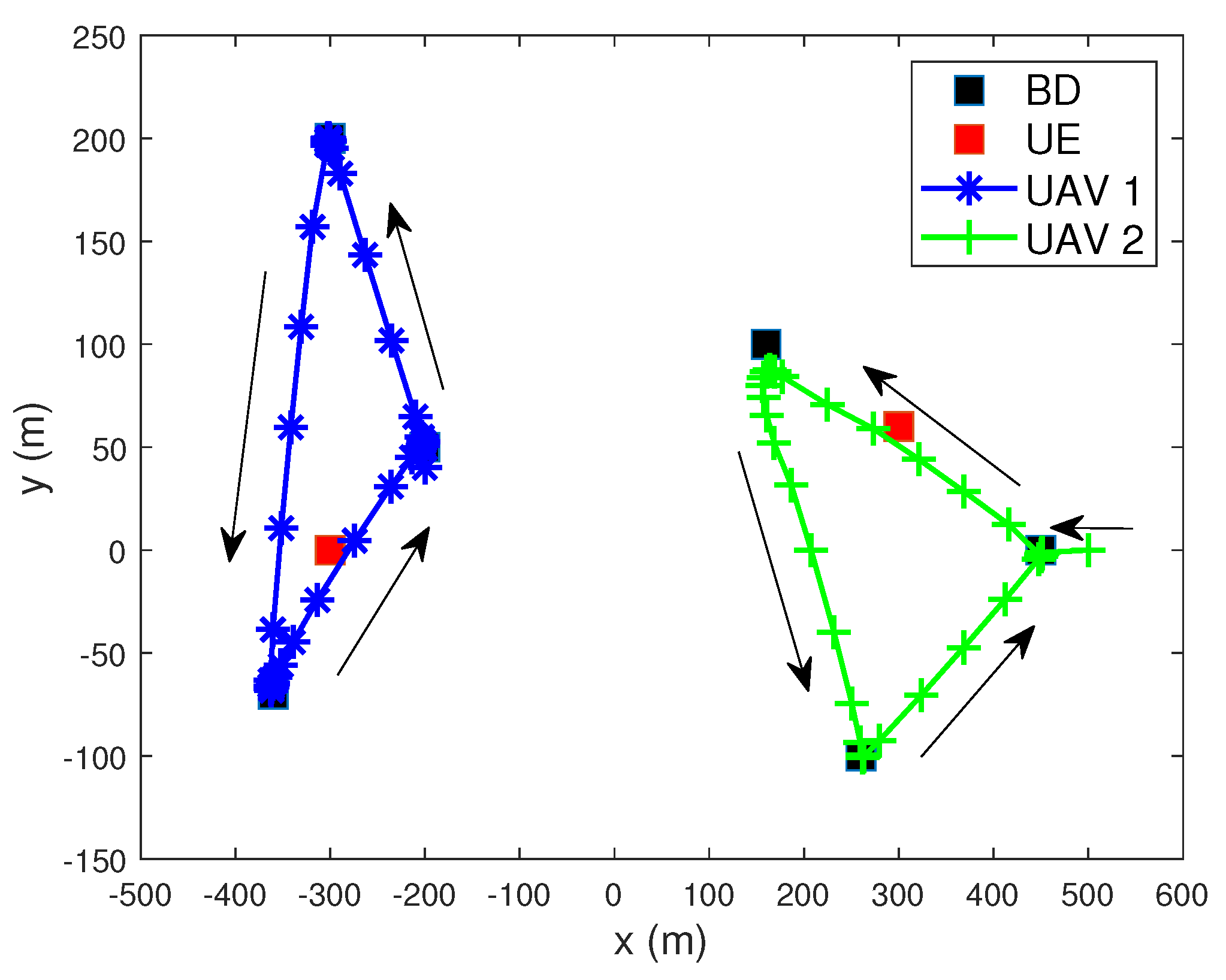
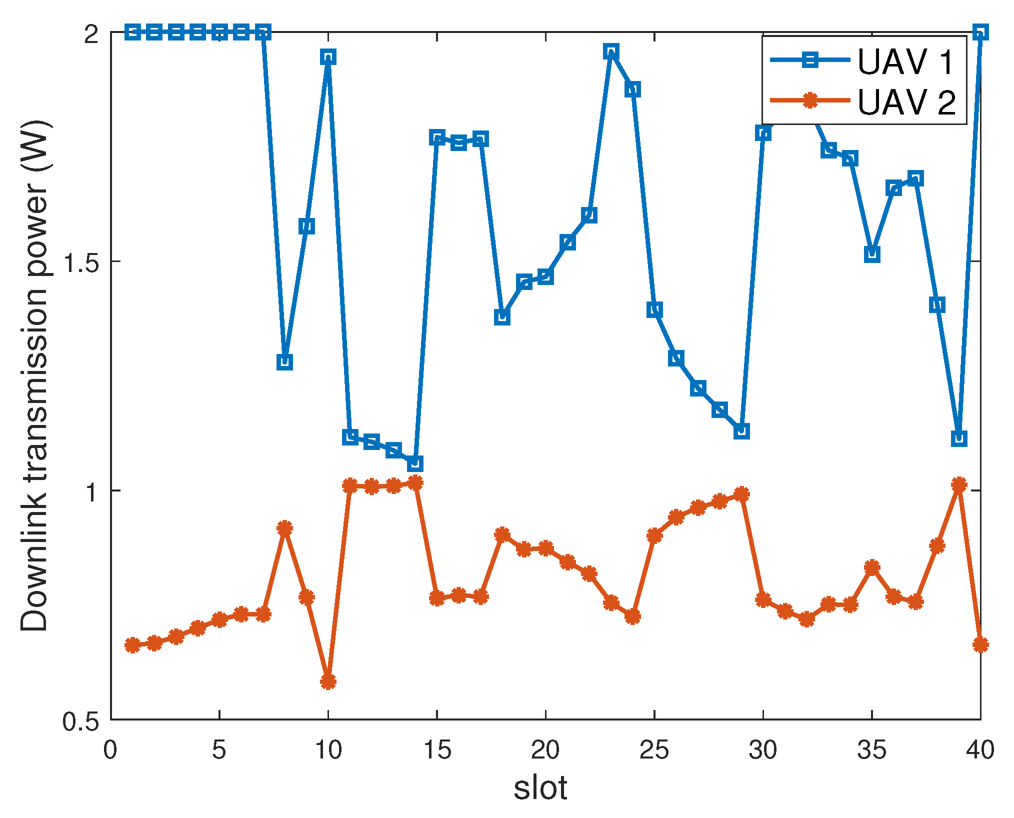
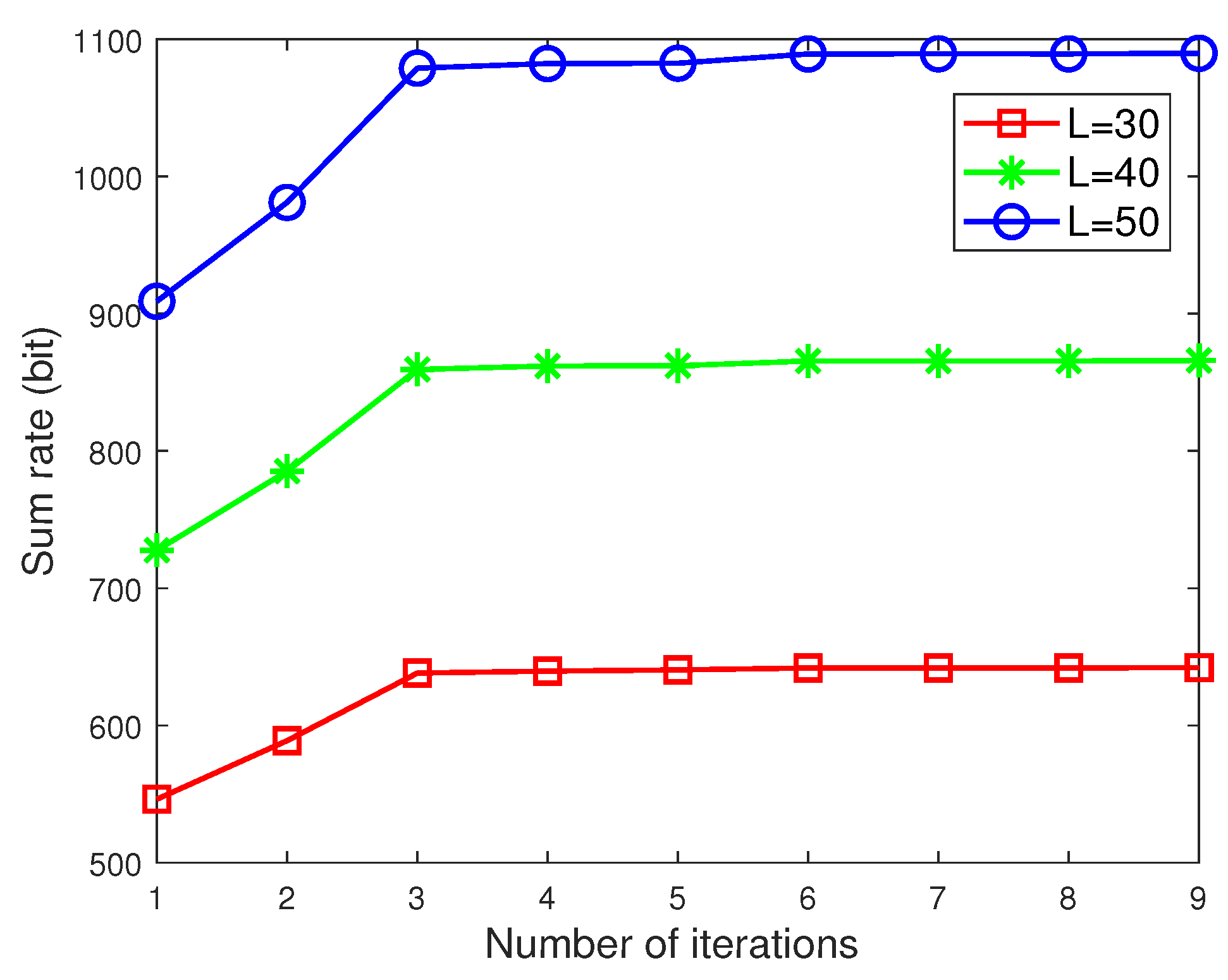
4. Simulation Results

In this section, we provide extensive numerical results to verify the efficiency of the proposed algorithm. We assume all the UEs and BDs are randomly distributed in the UAV service region. The location of the base station is (0,800,0). Unless otherwise stated, the remaining system parameters are listed in

Table 1. Simulation parameters.

Parameter	Value
Number of UAVs U	2
Number of UEs I	7
Number of BDs D	6
Number of slots Q	40
UAV’s maximum speed $V_{max}$	50 m/s
UAV’s maximum transmission power $P_{max}$	2 W
Noise power of UAV ${\sigma }_{\mathrm{u}}^2$ and the BD ${\sigma }_{\mathrm{b}}^2$	−144 dBm
Noise power of UE ${\sigma }_{\mathrm{u}}^2$ and the BS ${\sigma }_{\mathrm{B}}^2$	−144 dBm
Duration of each slot $\Delta t$	1 s
Carrier frequency for downlink $f_{c1}$	4 GHz
Carrier frequency for backhaul link $f_{c2}$	1 GHz
Height of UAV $h_{\mathrm{uav}}$	100
Attenuation coefficient of LoS ${\eta }_Q$	1 dB
Attenuation coefficient of NLoS ${\eta }_N$	20 dB
SINR threshold $\kappa$	0 dB
Minimum distance $d_{min}$	5 m

[21,22,23]. Furthermore, the initial transmission power of the UAV is evenly allocated for the downlink and the backhaul link. The BD reflection coefficient is set to 1.

In order to intuitively demonstrate the effect of the proposed algorithm, we display the optimized trajectory of the UAV in Figure 2. In Figure 2, the black squares and red squares represent the positions of BD and UE, respectively, and the trajectory of the UAV is plotted by the solid lines with different markers. The direction of the arrow represents the movement direction of the UAVs. It can be noted that in order to maximize the sum rate of the BDs, the UAV will traverse all the locations of the BD. Meanwhile, to keep the QoS of the UE, it will also approach the UE during the flight.

Figure 3 plots the optimized downlink transmission power of the UAV w.r.t. different slots. It can be noted that the downlink transmission power of UAV-1 is higher than that of UAV-2. This is because UAV-1 is closer to the BS, so it needs less backhaul transmission power to forward the data of BDs. Furthermore, as shown in Figure 3, the transmission power variation of the two UAVs is the opposite of satisfying the SINR constraint of the BD and the QoS constraint of the UE. When a UAV is close to the served BD, and another UAV is far away from the served BD, the farther away UAV will increase the transmission power to obtain a higher rate, while the closer UAV will decrease the transmission power to reduce interference to another BD and UE, thereby enhancing the sum rate with the constraint of the BD and UE satisfied.

To illustrate the superiority of the proposed algorithm, we consider two benchmark schemes: (1) OMA scheme, that is, the UAV can access only one BD at each slot with the proposed algorithm; (2) fixed location, that is, the UAV stays hovering. Figure 4 demonstrates the sum rate w.r.t. the number of slots. As shown in Figure 4, more service time increases the system’s sum rate. Furthermore, the performance of the proposed algorithm is better than that of the two fixed trajectory baseline algorithms, which shows the effectiveness of the proposed algorithm. Meanwhile, although the OMA scheme is also optimized with the same algorithm, its performance is still worse than that of the NOMA scheme, which shows the superiority of the NOMA scheme in the sum rate.

Figure 5 shows the sum rate w.r.t. the number of BDs. In the simulation, we keep the total service slots Q and the initial trajectory of the UAV unchanged. With the increase in the number of BDs, the sum rate performance of the four schemes will be improved. However, too much BD makes the improvement of the sum rate inefficient. This is because the increase in space density of BD reduces the freedom of UAV trajectory optimization. Meanwhile, the superiority of the proposed optimization algorithm and the NOMA scheme are also intuitively shown in Figure 5.

We demonstrate the impact of the height of the UAV on the system sum rate in Figure 6. It can be noted that the sum rate of all three schemes decreases as the height of the UAV increases. This is due to the fact that the altitude of the UAV affects the quality of the channel; that is, as the UAV increases its flight altitude, the distance from the UAV to the BD, the user, and the BS also increases, resulting in greater path loss. Therefore, the increase in the UAV height reduces the sum rate of the system. In addition, we can see that the proposed algorithm still outperforms the other two schemes, which verifies the effectiveness of the proposed algorithm again.

Finally, we demonstrate the convergence of the proposed algorithm in Figure 7. It can be observed that the proposed algorithm can reach the optimal state within three iterations under different slots, which verifies the faster convergence of Algorithm 1.

5. Conclusions

In this work, we investigated a multi-FD-UAV-assisted, NOMA-enabled backscatter communication network, where multiple FD UAVs were deployed to serve the downlink UEs and also collect the data reflected by the BDs with the NOMA scheme, and a BS provided the backhaul link of the UAV. Then, we formulated an optimization problem to maximize the sum rate of the BDs by jointly optimizing the reflection coefficient of BDs, the downlink and the backhaul transmission power, and the trajectory of UAVs. To solve this non-convex problem, we decomposed it into three independent sub-problems and adopted the SCA method to solve them. Based on the transformed sub-problems, we proposed a BCD-based iterative algorithm to tackle the original problem. The simulation results validate the superiority and the fast convergence of the proposed algorithm and the efficiency of the developed NOMA system with limited time-frequency resources.

References

1. Giordani, M.; Polese, M.; Mezzavilla, M.; Rangan, S.; Zorzi, M. Toward 6G Networks: Use Cases and Technologies. IEEE Commun. Mag. 2020, 58, 55–61. [Google Scholar] [CrossRef]
2. Pan, J.; Ye, N.; Yu, H.; Hong, T.; Al-Rubaye, S.; Mumtaz, S.; Al-Dulaimi, A.; Chih-Lin, I. AI-Driven Blind Signature Classification for IoT Connectivity: A Deep Learning Approach. IEEE Trans. Wirel. Commun. 2022, 21, 6033–6047. [Google Scholar] [CrossRef]
3. Ye, N.; Yu, J.; Wang, A.; Zhang, R. Help from space: Grant-free massive access for satellite-based IoT in the 6G era. Digit. Commun. Netw. 2022, 8, 215–224. [Google Scholar] [CrossRef]
4. Lu, X.; Niyato, D.; Jiang, H.; Kim, D.I.; Xiao, Y.; Han, Z. Ambient Backscatter Assisted Wireless Powered Communications. IEEE Wirel. Commun. 2018, 25, 170–177. [Google Scholar] [CrossRef]
5. Darsena, D.; Gelli, G.; Verde, F. Modeling and Performance Analysis of Wireless Networks With Ambient Backscatter Devices. IEEE Trans. Commun. 2017, 65, 1797–1814. [Google Scholar] [CrossRef]
6. Van Huynh, N.; Hoang, D.T.; Lu, X.; Niyato, D.; Wang, P.; Kim, D.I. Ambient Backscatter Communications: A Contemporary Survey. IEEE Commun. Surv. Tutor. 2018, 20, 2889–2922. [Google Scholar] [CrossRef] [Green Version]
7. Memon, M.L.; Saxena, N.; Roy, A.; Shin, D.R. Backscatter Communications: Inception of the Battery-Free Era—A Comprehensive Survey. Electronics 2019, 8, 129. [Google Scholar] [CrossRef] [Green Version]
8. Zhou, S.; Xu, W.; Wang, K.; Pan, C.; Alouini, M.; Nallanathan, A. Ergodic Rate Analysis of Cooperative Ambient Backscatter Communication. IEEE Wirel. Commun. Lett. 2019, 8, 1679–1682. [Google Scholar] [CrossRef] [Green Version]
9. Ye, Y.; Shi, L.; Chu, X.; Lu, G. On the Outage Performance of Ambient Backscatter Communications. IEEE Internet Things J. 2020, 7, 7265–7278. [Google Scholar] [CrossRef]
10. Han, D.; Minn, H. Coverage Probability Analysis Under Clustered Ambient Backscatter Nodes. IEEE Wirel. Commun. Lett. 2019, 8, 1713–1717. [Google Scholar] [CrossRef] [Green Version]
11. Van Huynh, N.; Hoang, D.T.; Niyato, D.; Wang, P.; Kim, D.I. Optimal Time Scheduling for Wireless-Powered Backscatter Communication Networks. IEEE Wirel. Commun. Lett. 2018, 7, 820–823. [Google Scholar] [CrossRef] [Green Version]
12. Wang, W.J.; Xu, K.; Yan, Y.; Chen, L. Relay Selection-Based Cooperative Backscatter Transmission With Energy Harvesting: Throughput Maximization. IEEE Wirel. Commun. Lett. 2022, 11, 1533–1537. [Google Scholar] [CrossRef]
13. Lyu, B.; You, C.; Yang, Z.; Gui, G. The Optimal Control Policy for RF-Powered Backscatter Communication Networks. IEEE Trans. Veh. Technol. 2018, 67, 2804–2808. [Google Scholar] [CrossRef]
14. Han, S.; Wang, Z. A Low-Complexity Resource Allocation for Multiple Access Passive IoT System. Electronics 2019, 8, 1421. [Google Scholar] [CrossRef] [Green Version]
15. Ye, Y.; Shi, L.; Chu, X.; Lu, G. Throughput Fairness Guarantee in Wireless Powered Backscatter Communications With HTT. IEEE Wirel. Commun. Lett. 2021, 10, 449–453. [Google Scholar] [CrossRef]
16. Yang, Z.; Feng, L.; Chang, Z.; Lu, J.; Liu, R.; Kadoch, M.; Cheriet, M. Prioritized Uplink Resource Allocation in Smart Grid Backscatter Communication Networks via Deep Reinforcement Learning. Electronics 2020, 9, 622. [Google Scholar] [CrossRef] [Green Version]
17. Li, L.; Huang, X. Promoting Energy Efficiency and Proportional Fairness in Densely Deployed Backscatter-Aided Networks. IEEE Internet Things J. 2021, 8, 10518–10530. [Google Scholar] [CrossRef]
18. Yang, H.; Ye, Y.; Chu, X. max–min Energy-Efficient Resource Allocation for Wireless Powered Backscatter Networks. IEEE Wirel. Commun. Lett. 2020, 9, 688–692. [Google Scholar] [CrossRef]
19. Zhang, Y.; Li, E.; Zhu, Y.H.; Chi, K.; Tian, X. Energy-Efficient Prefix Code Based Backscatter Communication for Wirelessly Powered Networks. IEEE Wirel. Commun. Lett. 2019, 8, 348–351. [Google Scholar] [CrossRef]
20. Liu, J.; Luo, Z.; Yang, G.; Liang, Y.C. Interference-Cancellation Transceiver Design for Long-Range Multistatic Backscatter Communications. In Proceedings of the GLOBECOM 2022–2022 IEEE Global Communications Conference, Rio de Janeiro, Brazil, 4–8 December 2022; pp. 6042–6047. [Google Scholar] [CrossRef]
21. Hua, M.; Yang, L.; Li, C.; Wu, Q.; Swindlehurst, A.L. Throughput Maximization for UAV-Aided Backscatter Communication Networks. IEEE Trans. Commun. 2020, 68, 1254–1270. [Google Scholar] [CrossRef] [Green Version]
22. Yang, G.; Dai, R.; Liang, Y.C. Energy-Efficient UAV Backscatter Communication With Joint Trajectory Design and Resource Optimization. IEEE Trans. Wirel. Commun. 2021, 20, 926–941. [Google Scholar] [CrossRef]
23. Yang, S.; Deng, Y.; Tang, X.; Ding, Y.; Zhou, J. Energy Efficiency Optimization for UAV-Assisted Backscatter Communications. IEEE Commun. Lett. 2019, 23, 2041–2045. [Google Scholar] [CrossRef] [Green Version]
24. Tran, D.H.; Chatzinotas, S.; Ottersten, B. Throughput Maximization for Backscatter- and Cache-Assisted Wireless Powered UAV Technology. IEEE Trans. Veh. Technol. 2022, 71, 5187–5202. [Google Scholar] [CrossRef]
25. Hu, J.; Cai, X.; Yang, K. Joint Trajectory and Scheduling Design for UAV Aided Secure Backscatter Communications. IEEE Wirel. Commun. Lett. 2020, 9, 2168–2172. [Google Scholar] [CrossRef]
26. Hua, M.; Swindlehurst, A.L.; Li, C.; Yang, L. UAV-Aided Backscatter Networks: Joint UAV Trajectory and Protocol Design. In Proceedings of the 2019 IEEE Global Communications Conference (GLOBECOM), Waikoloa, HI, USA, 9–13 December 2019; pp. 1–6. [Google Scholar] [CrossRef]
27. Farajzadeh, A.; Ercetin, O.; Yanikomeroglu, H. Mobility-Assisted Over-the-Air Computation for Backscatter Sensor Networks. IEEE Wirel. Commun. Lett. 2020, 9, 675–678. [Google Scholar] [CrossRef] [Green Version]
28. Nie, Y.; Zhao, J.; Liu, J.; Jiang, J.; Ding, R. Energy-efficient UAV trajectory design for backscatter communication: A deep reinforcement learning approach. China Commun. 2020, 17, 129–141. [Google Scholar] [CrossRef]
29. Liu, Q.; Sun, S.; Hou, J.; Jia, H.; Kadoch, M. Resource Allocation in NOMA-Assisted Ambient Backscatter Communication System. Electronics 2021, 10, 3061. [Google Scholar] [CrossRef]
30. Yang, G.; Xu, X.; Liang, Y.C. Resource Allocation in NOMA-Enhanced Backscatter Communication Networks for Wireless Powered IoT. IEEE Wirel. Commun. Lett. 2020, 9, 117–120. [Google Scholar] [CrossRef]
31. Chen, W.; Ding, H.; Wang, S.; da Costa, D.B.; Gong, F.; Nardelli, P.H.J. Ambient backscatter communications over NOMA downlink channels. China Commun. 2020, 17, 80–100. [Google Scholar] [CrossRef]
32. Khan, W.U.; Li, X.; Zeng, M.; Dobre, O.A. Backscatter-Enabled NOMA for Future 6G Systems: A New Optimization Framework Under Imperfect SIC. IEEE Commun. Lett. 2021, 25, 1669–1672. [Google Scholar] [CrossRef]
33. Ding, Z.; Poor, H.V. On the Application of BAC-NOMA to 6G umMTC. IEEE Commun. Lett. 2021, 25, 2678–2682. [Google Scholar] [CrossRef]
34. Farajzadeh, A.; Ercetin, O.; Yanikomeroglu, H. UAV Data Collection Over NOMA Backscatter Networks: UAV Altitude and Trajectory Optimization. In Proceedings of the ICC 2019–2019 IEEE International Conference on Communications (ICC), Shanghai, China, 20–24 May 2019; pp. 1–7. [Google Scholar] [CrossRef] [Green Version]
35. Gan, X.; Jiang, Y.; Wang, Y.; Hong, D.; Wang, Z. Sum Rate Maximization for UAV-assisted NOMA Backscatter Communication System. In Proceedings of the 2023 6th World Conference on Computing and Communication Technologies (WCCCT), Chengdu, China, 6–8 January 2023; pp. 19–23. [Google Scholar] [CrossRef]
36. Fan, Z.; Hu, Y.; Wang, Z.; Wan, X.; Duo, B. Sum Rate Optimization for UAV-assisted NOMA-based Backscatter Communication System. In Proceedings of the 2022 27th Asia Pacific Conference on Communications (APCC), Jeju Island, Republic of Korea, 19–21 October 2022; pp. 478–482. [Google Scholar] [CrossRef]
37. Liu, V.; Parks, A.N.; Talla, V.; Gollakota, S.; Wetherall, D.J.; Smith, J.R. Ambient backscatter: Wireless communication out of thin air. ACM SIGCOMM Comput. Commun. Rev. 2013, 43, 39–50. [Google Scholar] [CrossRef]
38. Wang, N.; Li, F.; Chen, D.; Liu, L.; Bao, Z. NOMA-Based Energy-Efficiency Optimization for UAV Enabled Space-Air-Ground Integrated Relay Networks. IEEE Trans. Veh. Technol. 2022, 71, 4129–4141. [Google Scholar] [CrossRef]
39. Ma, T.; Zhou, H.; Qian, B.; Cheng, N.; Shen, X.; Chen, X.; Bai, B. UAV-LEO Integrated Backbone: A Ubiquitous Data Collection Approach for B5G Internet of Remote Things Networks. IEEE J. Sel. Areas Commun. 2021, 39, 3491–3505. [Google Scholar] [CrossRef]
40. Ding, Z.; Poor, H.V. Advantages of NOMA for Multi-User BackCom Networks. IEEE Commun. Lett. 2021, 25, 3408–3412. [Google Scholar] [CrossRef]
41. Wu, Q.; Zeng, Y.; Zhang, R. Joint Trajectory and Communication Design for Multi-UAV Enabled Wireless Networks. IEEE Trans. Wirel. Commun. 2018, 17, 2109–2121. [Google Scholar] [CrossRef] [Green Version]
42. Lu, J.; Wang, Y.; Liu, T.; Zhuang, Z.; Zhou, X.; Shu, F.; Han, Z. UAV-Enabled Uplink Non-Orthogonal Multiple Access System: Joint Deployment and Power Control. IEEE Trans. Veh. Technol. 2020, 69, 10090–10102. [Google Scholar] [CrossRef]
43. Liu, X.; Lai, B.; Lin, B.; Leung, V.C.M. Joint Communication and Trajectory Optimization for Multi-UAV Enabled Mobile Internet of Vehicles. IEEE Trans. Intell. Transp. Syst. 2022, 23, 15354–15366. [Google Scholar] [CrossRef]
44. Zhan, C.; Hu, H.; Liu, Z.; Wang, Z.; Mao, S. Multi-UAV-Enabled Mobile-Edge Computing for Time-Constrained IoT Applications. IEEE Internet Things J. 2021, 8, 15553–15567. [Google Scholar] [CrossRef]
Figure 1. Multi-FD-UAV-assisted NOMA-enabled backscatter communication network.
Electronics 12 01873 g001
Figure 2. Optimized UAV trajectory.
Electronics 12 01873 g002
Figure 3. Optimized UAV downlink transmission power.
Electronics 12 01873 g003
Figure 4. The sum rate w.r.t. the number of slots.
Electronics 12 01873 g004
Figure 5. The sum rate w.r.t. the number of BDs.
Electronics 12 01873 g005
Figure 6. The sum rate w.r.s. the height of UAVs.
Electronics 12 01873 g006
Figure 7. The sum rate w.r.t. the number of iterations.
Electronics 12 01873 g007