1. Introduction
The Shack–Hartmann wavefront sensor (SHWFS) is one of the most widely used wavefront sensors (WFSs) in adaptive optics (AO) systems [
1]. The micro lenslet array (MLA) samples the input wavefront spatially, and by determining the local slope on each sub-aperture, the entire wavefront can be reconstructed successively. The local slopes over individual sub-apertures are calculated linearly from the displacements of spots focused by the micro lenses from their optical axes. Therefore, the accuracy of the spot displacement estimation is directly related to the overall performance of the SHWFS, as error from the estimation will pass through various stages to the final wavefront reconstruction stage. Center of Gravity (CoG)-based methods have been largely used for determining the centroids of the spots by measuring the center of mass within a window associated to a particular micro lenslet. Matched filter [
2], minimum mean-square-error estimator [
3], and maximum-likelihood methods [
4] have been studied to estimate the centroid or wavefront slope as well. If the source is an extended object instead of a point source, cross-correlation methods can also be used to estimate the sub-image displacement [
5,
6,
7]. A comparison of some commonly used centroiding algorithms, including thresholding (TCoG), weighted centroid (WCoG), correlation, and quad cell, is given by Thomas et al. [
8]. For closed-loop AO systems and fast wavefront sensing, the CoG-based methods are still preferred over other methods due to their robustness and easy implementation.
Conventional CoG estimations are often corrupted due to various noise sources such as photon noise, readout noise of the image sensor, and the finite and coarse sampling of the pixels. These CoG-derived methods also fail to estimate the local wavefront if the spot breaks into parts due to strong turbulence with lower Fried coherence length
or when scintillation from distant volumes of turbulence is presented. Using Gaussian approximation, Rousset [
9] pointed out that the noise variance in local wavefront estimation due to sensor readout noise increases with the increased number of pixels for CoG calculation. On the other hand, Irwan et al. showed that the error variance due to photon noise also diverges as detector size increases, even for a perfect CCD array, and even without readout noise and effects due to finite pixel size. These analyses mean that a small CoG calculation window is necessary in order to reduce the error contribution of photon and sensor readout noise. However, if the window for the CoG calculation is too small, signal truncation error will be introduced when the spot moves to the window edge, which in turn leads to a limited dynamic range of the SHWFS. Therefore, the optimal CoG calculation window size often needs to balance between the noise errors and dynamic range. To isolate the useful signal for CoG calculation, the traditional CoG methods have been improved by thresholding the signal [
10,
11] or adding weight to emphasize the signal [
12,
13]. The error sources for centroid computation of a point source on a CCD-based sensor were analyzed by Ma et al. [
14] and the best threshold level is given. Other methods using iterative detection of spot location and centroid estimation have been reported [
15,
16]. While they improve the best area for the CoG calculation, these iterations will introduce extra delay for the centroid measurements and eventually reduce the bandwidth of a closed-loop AO system. Recent efforts to improve the performance of Shack–Hartmann WFS include direct wavefront reconstruction as a continuous function from a bitmap image of the Shack–Hartmann pattern [
17], and using artificial neural networks [
18] and learning-based methods [
19] for spot detection. To overcome the limitation of Shack–Hartmann WFS in certain situations, e.g., under strong scintillation, a diffractive lenslet array can also been used to replace the physical MLA, leading to a more flexible and adaptable Shack–Hartamnn WFS [
20]. Talmi and Ribak [
21] showed that gradient calculation over the whole aperture is possible by direct demodulation on the grid without reverting to Fourier Transforms. This method is especially suited to very large arrays due to the saving of computation by removing the two inverse Fourier Transforms. Importantly, they considered that incomplete spots, for example, at the edge of the aperture, would create bias on the complete reconstruction, and showed that processing these in a sensible way in the image domain could have a lesser effect on the whole reconstruction.
In addition to the effort to improve the accuracy of centroid estimation algorithms, other researchers also tried to increase the wavefront sensing speed by utilizing special hardware such as GPU [
22,
23] or field-programmable gate array (FPGA) devices for implementation. For example, FPGA devices have been used both in complex AO systems to process data where the timing is crucial [
24,
25,
26], or used to implement centroid estimation and reconstruction [
27,
28,
29], or even to develop full AO application including driving the wavefront corrector [
30,
31]. In comparison with conventional CPU [
32] or GPU-based solutions, FPGA devices provide a cost-effective way to achieve a high throughput, low latency and reconfigurable wavefront sensing, and AO system thanks to their parallel computation power.
In our previous work [
33], we proposed an improved stream-based center of gravity (SCoG) method for centroid estimation which is suitable to be implemented on FPGA devices. By extending the conventional CoG method to evaluate the center of gravity around each incoming pixel, the SCoG method can use an optimal CoG window matching the size of the spot behind the MLA without the common trade-off between increased bias error and reduced noise errors. In addition, the accuracy of the centroid estimation by SCoG is not compromised when the spot moves to the sub-aperture edge or even crosses the boundary, since the CoG operation centers on each individual pixel. The SCoG is also able to detect multiple centroids within one sub-aperture when the size of the CoG window is chosen appropriately because of its whole sensor centroid calculation.
While complicated and advanced CoG methods [
12,
13,
15,
17] have been proposed to improve the accuracy of the centroid estimation, little work has been reported to discuss their appropriate implementations to meet the low latency and high bandwidth requirement in real-time AO systems. However, most real-time implementations of the Shack–Hartmann WFS [
22,
23,
28,
32] use the basic thresholding CoG method. In this paper, we present a complete Shack–Hartmann wavefront sensing system implemented on FPGA hardware with very low latency and high accuracy using the superior SCoG for centroid estimations. A parallel slope calculation and a robust least-squares wavefront reconstruction are also implemented in a pipe-lined way after the centroid estimation. The paper is organized as follows: In
Section 2, the theory of stream-based center of gravity deriving from conventional CoG methods, special treatments of multiple or missing centroids in sub-apertures, and the modal wavefront reconstruction are explained. The hardware implementations of the SCoG module, centroids segmentation module, and least-square modal wavefront reconstruction module are described in detail in
Section 3. In
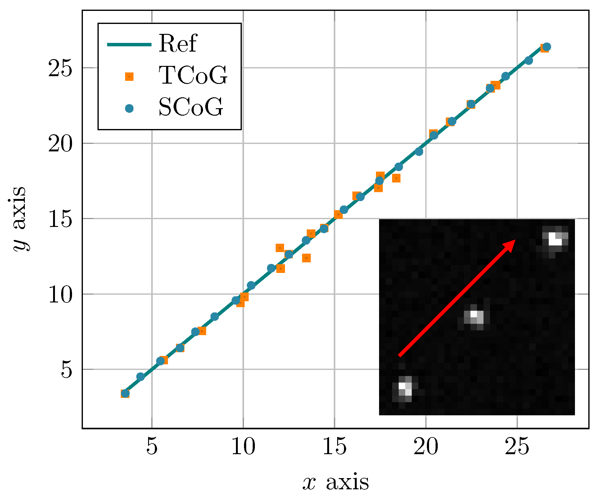
Section 4, the resource usage and latency of the FPGA implementation are analyzed. Performance of the centroiding algorithm is compared with a traditional CoG method using an artificially generated image of spots followed by an examination of the wavefront reconstruction performance of the whole Shack–Hartmann WFS system. Conclusions and future work are summarized in
Section 5.
2. Theoretical Background
Some notations used in this section to describe the stream-based center of gravity algorithm are listed in
Table 1.
2.1. Conventional Center of Gravity
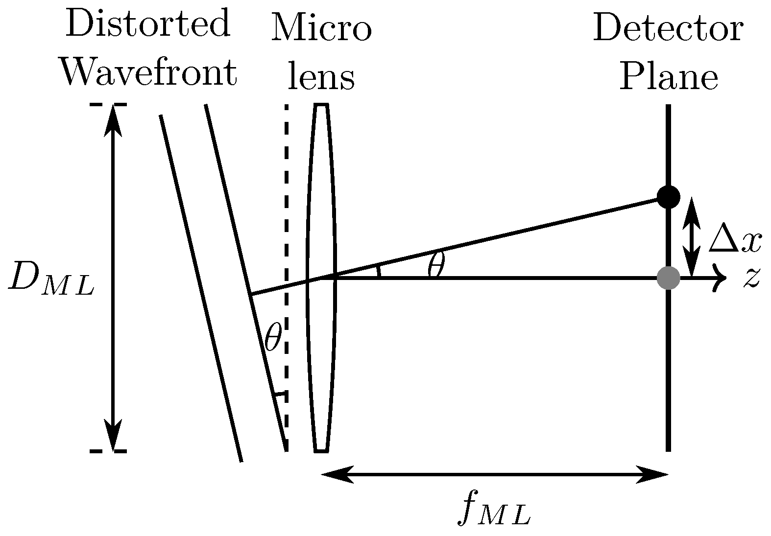
The geometric diagram of a single lenslet from a MLA is shown in
Figure 1. The local wavefront tilt
in a sub-aperture
causes a shift
of the focal spot from its reference on-axis position
when a plane wavefront is used. The size of the diffraction-limited spot is determined by the f-number of the lenslet and equals to
where
and
are the focal length and diameter of the micro lens respectively. By determining the local slopes at all sub-apertures, a continuous wavefront map can be reconstructed using either zonal- or modal-based reconstruction methods.
The local slope over sub-aperture
can be calculated by:
where
,
are the displacement of the spot in
x and
y directions from its reference location.
Figure 1.
Schematic of a single micro lens in the Shack–Hartmann wavefront sensor.
Figure 1.
Schematic of a single micro lens in the Shack–Hartmann wavefront sensor.
In Equation (2), the centroid in the sub-aperture
can be measured in
x and
y directions using the traditional CoG definition as:
where
is the coordinate of the sub-aperture,
is pixel index, and
is the pixel intensity. In a traditional instrument, the CoG is only calculated on the central pixel location
per lenslet.
2.2. Stream-Based Center of Gravity
The conventional CoG method can be extended by evaluating the centroid estimation on each pixel of the signal:
where
is a linear filter ranging from
to
M.
represents the estimated centroid value for the pixel
within a square window of side size of
.
If the centroid estimation value at a pixel equals to zero, then a spot is centered on this pixel. In most cases, however, the centroid is less likely to sit on an exact pixel but rather between two pixels. A potential spot is detected around pixel if a zero-crossing (from positive to negative) of CoG values happens horizontally between pixels and and vertically between pixels and at the same time.
The sub-pixel shift in the
x directions from pixel
can be interpreted linearly by the CoG values at pixel
and its left pixel
, while the sub-pixel shift in
y direction can be interpreted similarly by the CoG values at pixel
and its above pixel
:
Therefore, the
th centroid
where a potential spot is located can be described by
as below:
Note that the calculation of integer and decimal parts of centroid are through separate steps and the integer parts, i.e., pixel indices, are determined first. can be obtained directly by the sign changes of the numerators in Equation (3) as the denominators which represent the sum of energy within the kernel window are always positive. If only whole pixel resolution is concerned, calculations of the numerators are sufficient to locate the pixel indices.
In this work, an estimate of centroid is made based on each and every pixel streamed from the image sensor, for which best centroids are tagged resulting in a stream of centroids or SCoG synchronous with the stream of pixels. Several immediate advantages of SCoG over conventional CoG-based centroid estimation methods can be noticed [
33]. Since the CoG window is floating with the incoming pixels and will center around each potential genuine centroid, bias errors due to asymmetric CoG filter are largely avoided. In addition, the size of the CoG window
can be optimised by matching with the diffraction-limited spot size to minimize the influence of irrelevant pixels so that noise errors are minimised.
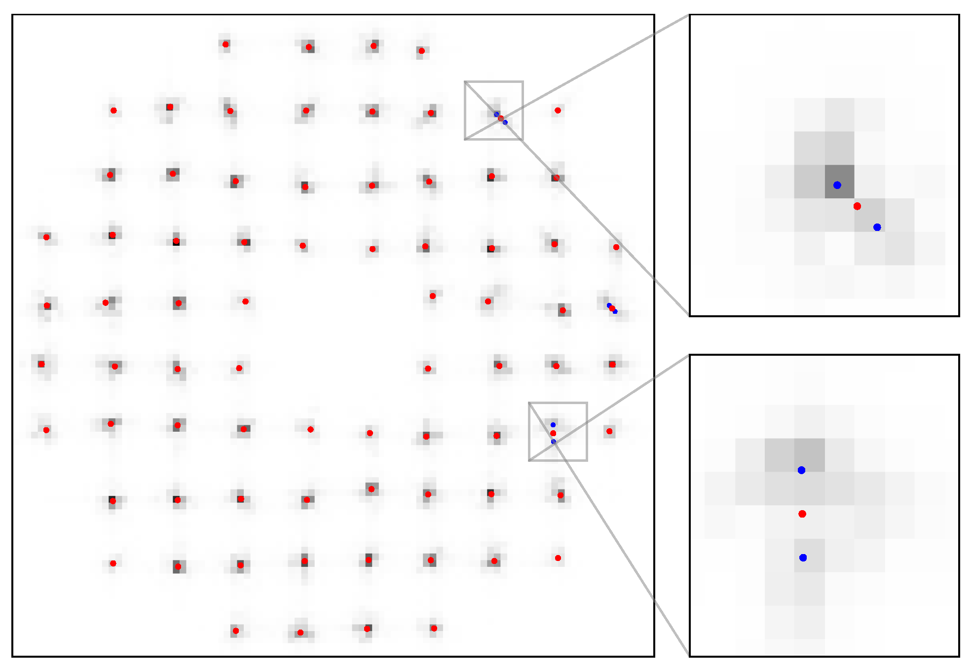
It is worth noting the unique characteristics of the centroids detected by the stream-based CoG algorithm. Using conventional sub-aperture-based CoG methods, only one centroid will be estimated for each sub-aperture, even when multiple spots exist due to, for example, binary star structure or strong turbulence, resulting in a “broken” spot ( is less than the microlens diameter). In addition, the measured centroids belonging to each sub-aperture are rather apparent from conventional CoG methods. However, the stream of centroids from SCoG arises in order based on the position of the spot occurrence in the input image frame as it is read from the image sensor, row-by-row, and column-by-column. Therefore, the SCoG centroids stream need to be further processed in order to be used in the conventional zonal or modal wavefront reconstruction algorithms.
2.3. Segmentation of the Streamed Centroids
There are two problems that need to be addressed for the stream of centroids
in order to get the centroid estimation for each sub-aperture associated with traditional CoG-based methods. First, the occurrence of centroid
follows the lower row number to a higher row number or a lower column number to a higher column number depending on the pixel reading sequence of the particular sensor. For a particular centroid
, it needs to be assigned to a sub-aperture
if its values are within the window of
defined by:
where
is the floor operation and
w is the window width in pixels.
Secondly, it is possible that multiple centroids or no valid centroid are detected within one sub-aperture , perhaps because of multiple objects, obstruction, or scintillation. For the multiple centroids case, different strategies can be used, such as using the centroid with the highest energy (sum of intensity as the denominator in Equation (3)) or taking the average of all centroids.
In our current implementation, we used the average of all centroids in the sub-aperture, hence effectively measuring the G-tilt of the local wavefront:
where
denotes the average operation and ∈ means the integer part of
that falls within the pixel range of sub-aperture
.
On the other hand, if a centroid is missing in a sub-aperture , it is possible to generate an average one from its surrounding sub-apertures. However, if one or more surrounding sub-apertures also miss valid centroids, the chain of average operation will expand to further sub-apertures which could soon become too complicated to manage. The other method to treat the sub-aperture with missing centroid is to inherit the corresponding centroid from a previous frame, which could be traced back to an original reference centroid if none of the previous frames contain a valid centroid.
Once all the valid sub-apertures in one MLA row have been processed to select a representative centroid estimation, they need to be re-ordered to match the sequence of the physical geometry, so the following wavefront reconstruction can be started even though the remaining lenslets have not yet arrived. Therefore, the further processing of the streamed centroids follows a sorting–processing–reordering procedure.
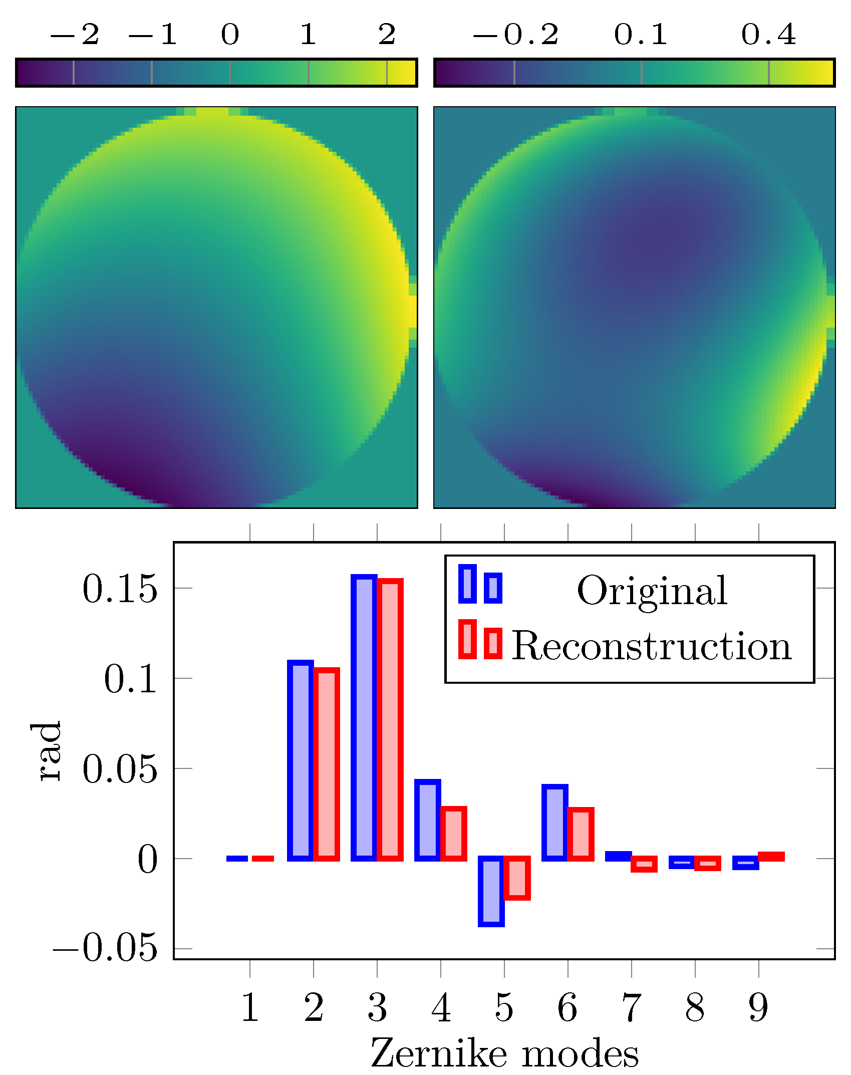
2.4. Wavefront Reconstruction
From the discrete slopes at all the valid sub-apertures as given by Equation (1), a continuous wavefront map can be reconstructed using
zonal,
modal, or
FFT-based methods [
34,
35]. Using the modal wavefront reconstruction, the incoming wavefront
over the pupil can be decomposed by a set of orthogonal functions, such as Zernike polynomials:
where
represents the weight of the
kth Zernike term
and
N is the total number of Zernike modes used to approximate the actual wavefront.
In Equation (1), the local slope of wavefront on the individual sub-apertures is expressed as a relation between the local sub-image displacements for each axis (
) and the MLA focal length
. Considering only the
x axis results in the following equation:
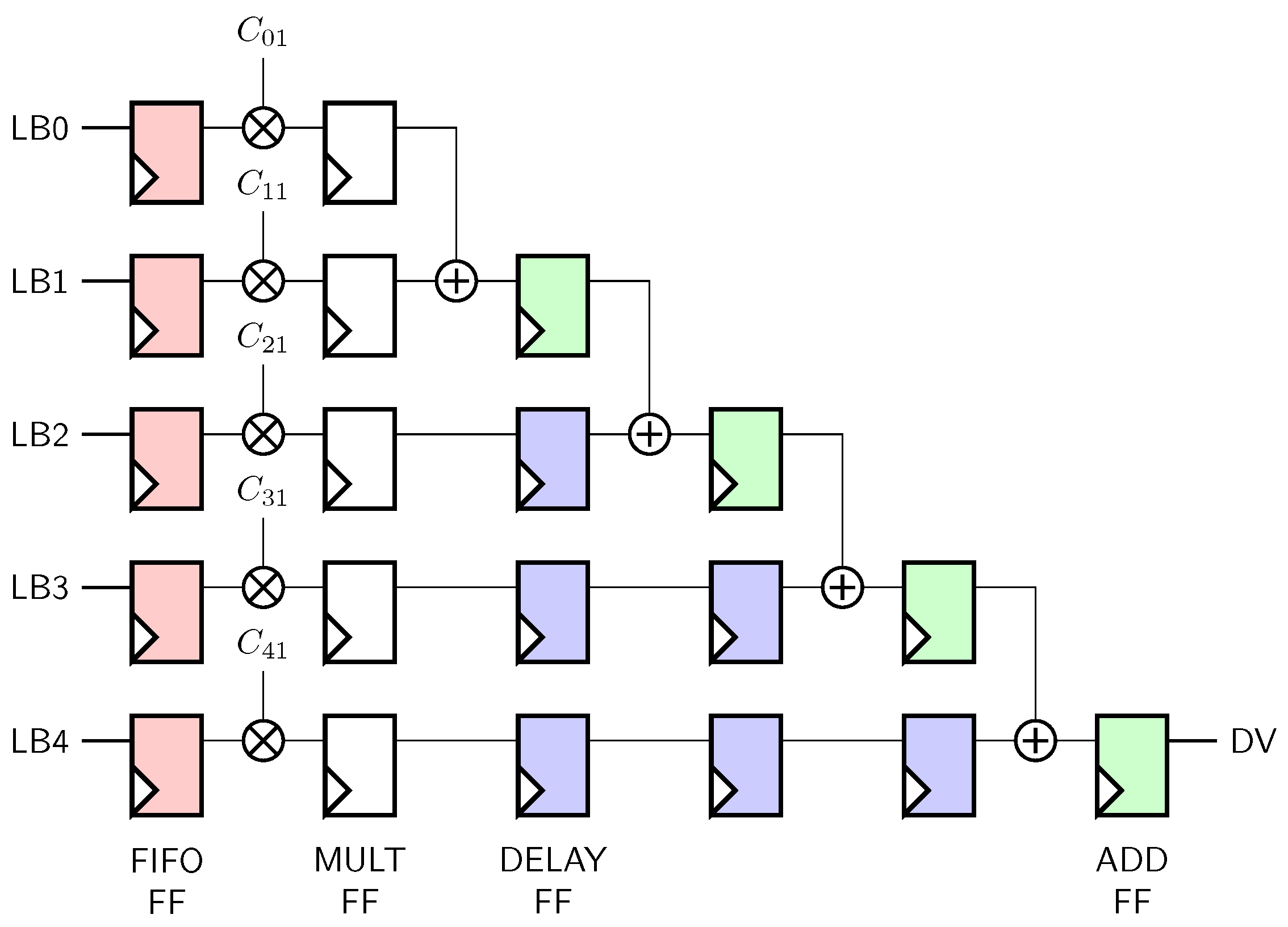
By combining Equations (9) and (10), the gradients of the wavefront over each sub-aperture can be related with a weighted sum of Zernike polynomials as follows:
Considering the slopes in both
x and
y directions for all the sub-apertures, Equation (11) can be expressed in the following matrix form:
where
M is the total number of valid sub-apertures and
N is the number of Zernike modes used for wavefront reconstruction.
is the slope vector of dimensions
and
is the Zernike mode coefficients vector of dimension
.
is a matrix of dimension
whose elements are the partial derivative of a Zernike mode on either
x or
y direction. Equation (12) defines
linear equations. To obtain the Zernike coefficients vector
from measured slope vector
, the pseudo-inverse of matrix
is used:
The pseudo-inverse matrix
, also known as the calibration matrix, has a dimension of
and can be calculated using the least squares estimation method:
In
Section 3.4, the detailed implementation of the modal wavefront reconstruction is explained.
3. Implementation
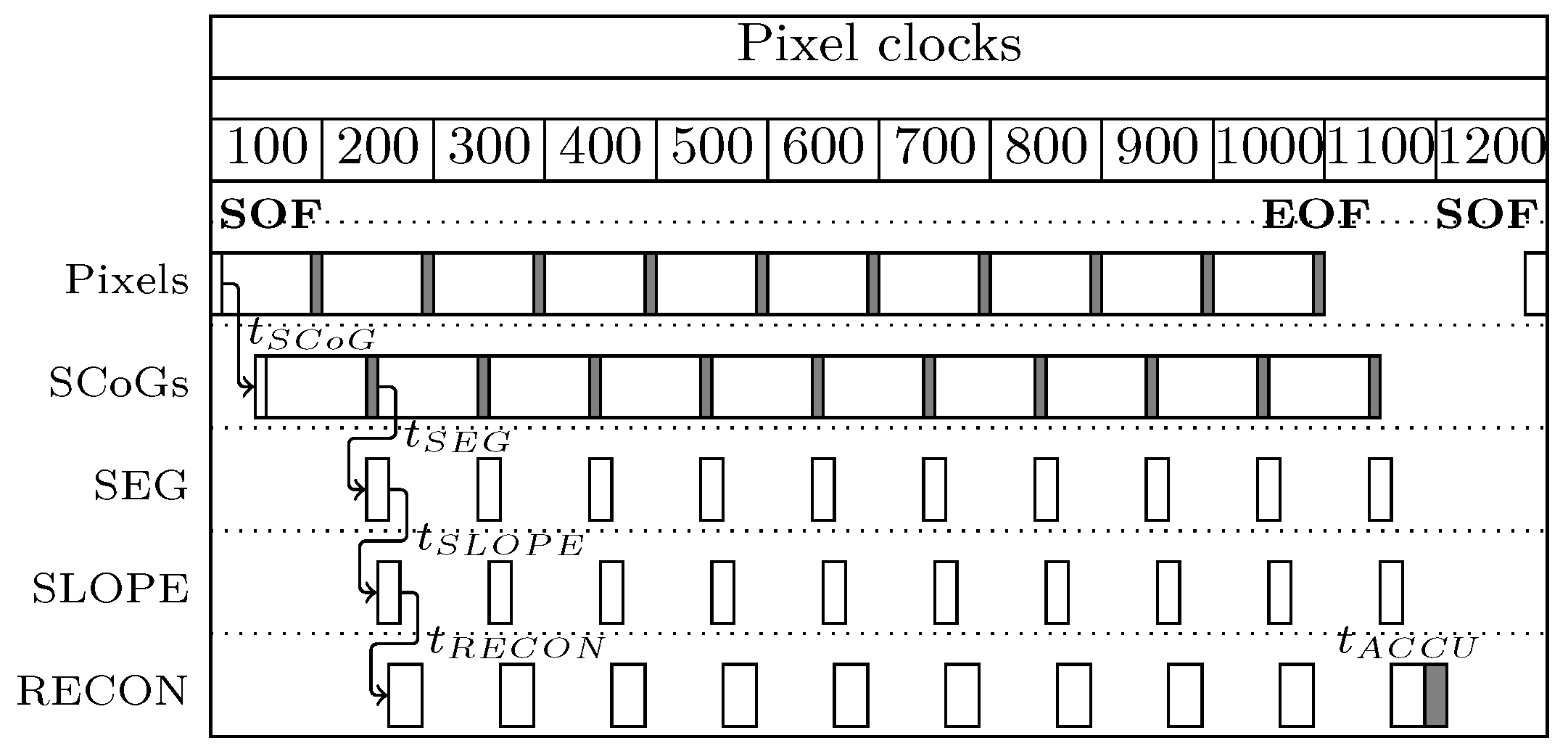
In this section, a parallel implementation of the stream-based center of gravity algorithm and the modal wavefront reconstruction suitable for FPGA devices are described. By taking advantage of parallelism and storage resources of FPGA devices, the CoG operation can be evaluated at each incoming pixel in real-time. The wavefront reconstruction can also start partially as soon as the centroids estimation of sub-apertures becomes available and complete at a very short delay after acquiring one image frame (and certainly before the start of the next frame).
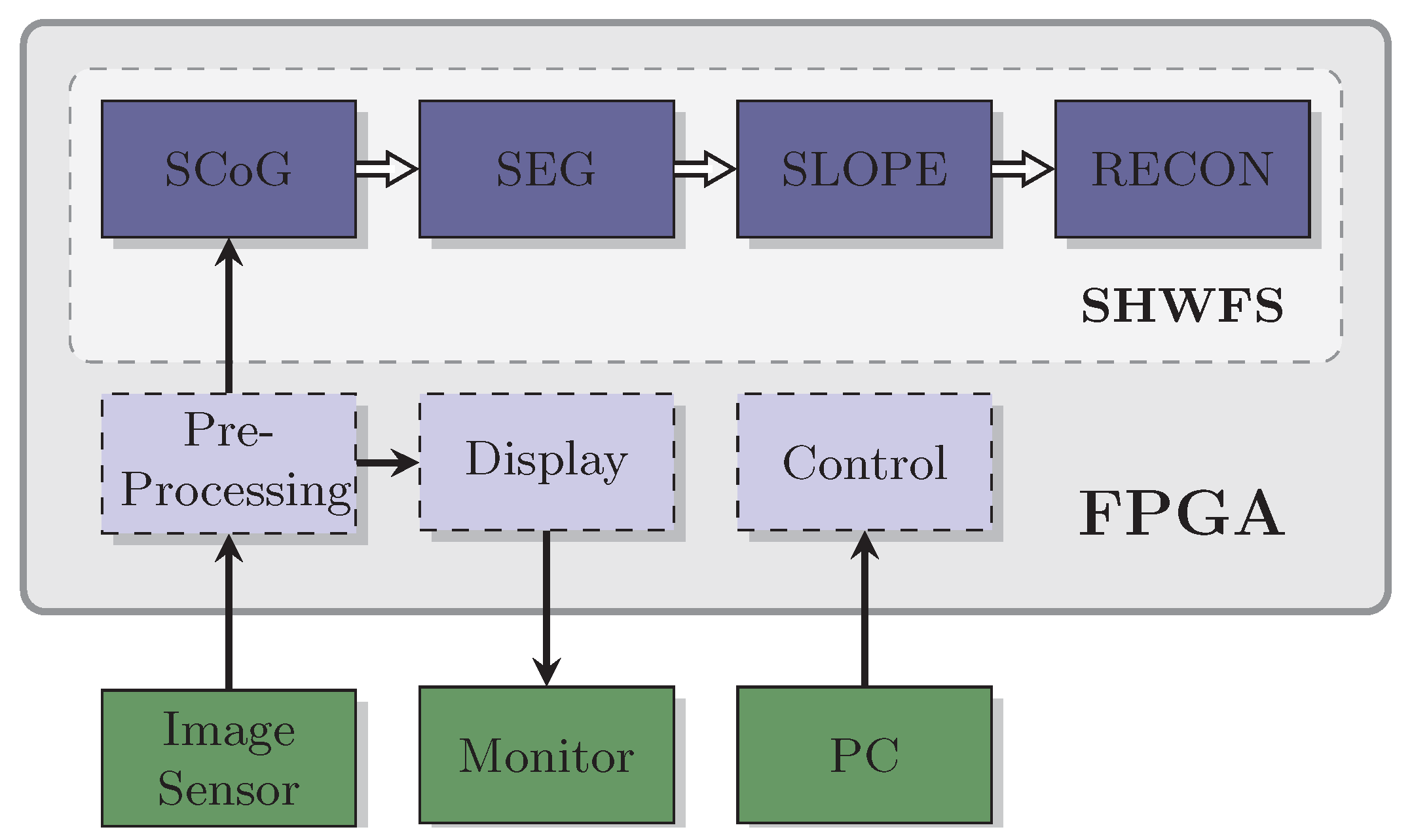
The overall block diagram of the SHWFS system design using the stream-based CoG method is shown in
Figure 2. The complete implementation consists of four main modules corresponding to
Section 2.2,
Section 2.3 and
Section 2.4:
SCoG module computes centroid on all incoming pixels and presents a stream of valid centroids;
SEG module sorts the centroids to confined sub-apertures and handles multiple centroids or centroids missing in some sub-apertures;
SLOPE module calculate the local slopes from measured centroids and can also be used to generate a reference centroid grid;
RECON module conducts a modal wavefront reconstruction from the measured slopes. The SCoG and SEG modules together provide similar functions to other conventional CoG methods. The auxiliary pre-processing, display, and control modules shown in light blue blocks are necessary to configure the image sensor, set system parameters, and visualize various results but not directly related to the research interest and therefore are omitted in the following discussion.
3.1. SCoG Module
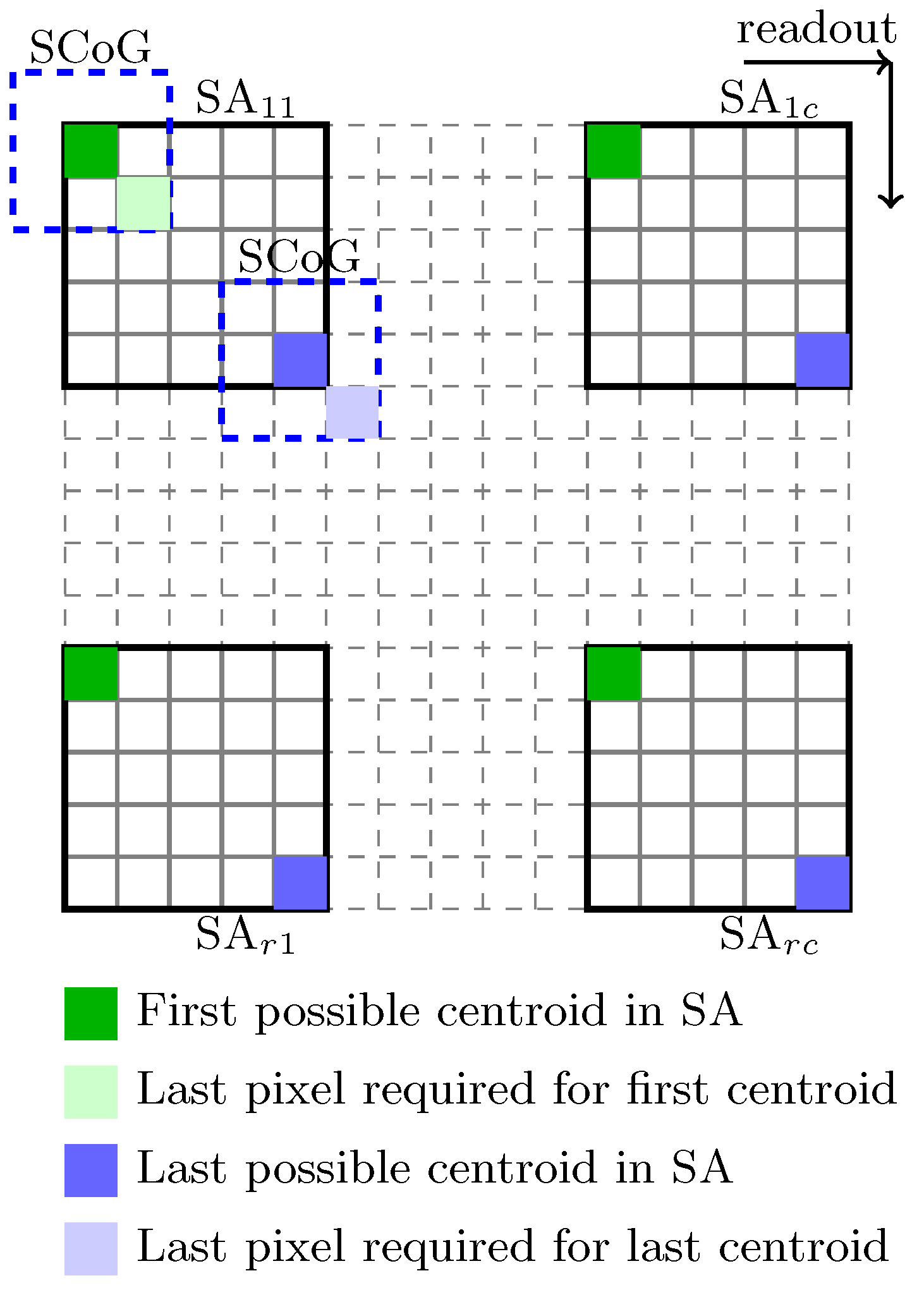
In
Figure 3, the 2D pixel array of an image sensor at the focal plane of the MLA is shown. The sub-aperture window SA corresponds to individual lenslet with its size and number of pixels (
for this example) determined by the lenslet and pixel sizes. Traditional CoG-based methods use all the pixels (except for the windowing CoG) inside the SA window for the calculation and generally need to read the whole image frame before computation. The SCoG operates on a much smaller pixel set (the blue dashed window) which could be optimized by matching the window with the spot size (
for this example). In the FPGA devices, First-In, First-Out (FIFO), or Look Up Table (LUT) can be used to buffer several rows and columns of pixels, so as the last required pixel arrives (light green and light blue pixel for the first and last possible centroids in
), the computation of the CoG will start.
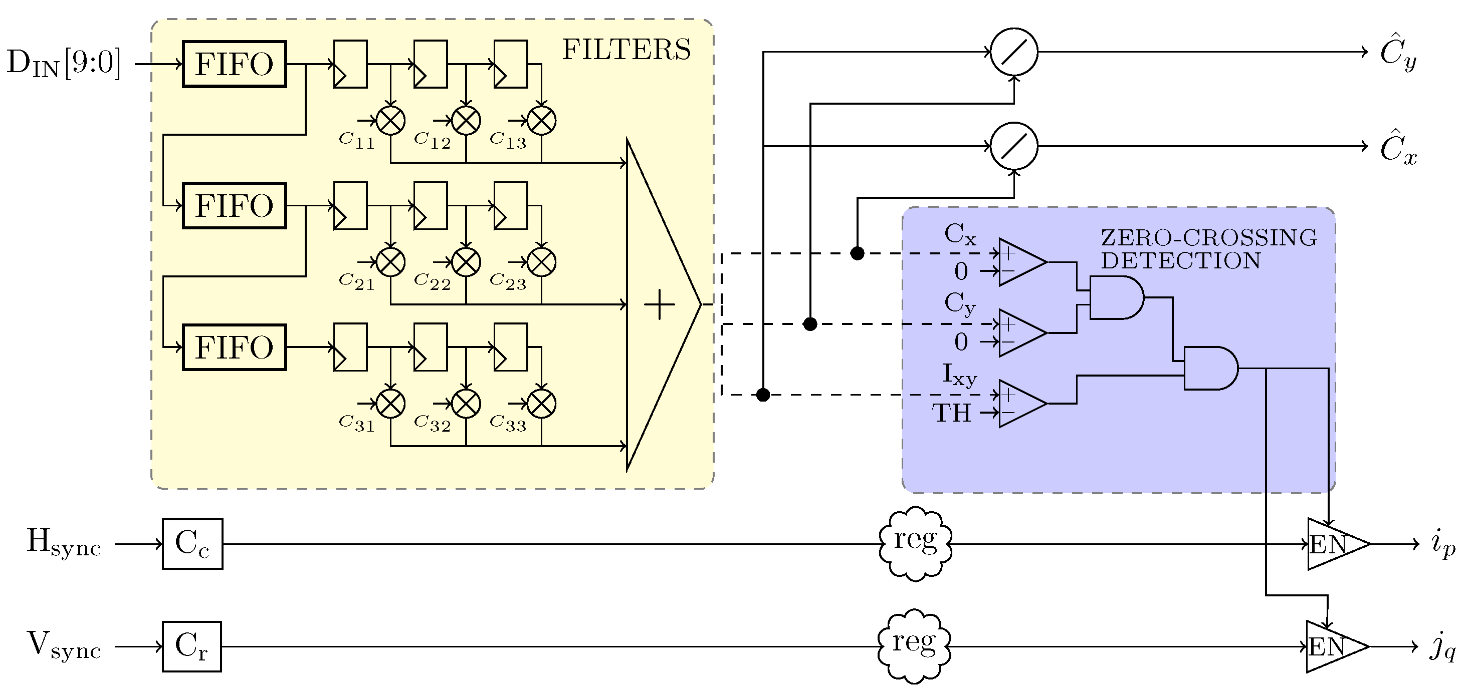
A high level logic diagram for calculating the stream centroid according to
Section 2.2 on each incoming pixel is shown in
Figure 4, where pixel Data
is synchronous with the master clock. The circuit in the yellow box represents a 2D convolution operation and it calculates either the numerators or denominators in Equation (3) depending on the chosen coefficients
to
in the multipliers, which represent the matrix elements in Equation (4). The SCoG window is assumed with a
size, and therefore three buffers are used to store three rows of pixel values and three Flip-Flop (FF) registers are used to buffer three columns of pixels. As the last required pixel within the SCoG window arrives at the output of the first buffer, all the required pixel values will appear at the nine registers’ output simultaneously at the next clock cycle. This implementation makes logical sense but is impractical, as all the multiplications and additions need to be finished in one clock cycle. This causes challenges to meeting timing constraints in FPGA implementation. In
Appendix A, matrix multiplication is separated to two 1D filter operations, which reduces the usage of multipliers. Furthermore, the implementation of the two 1D filter operations are fully pipe-lined to best improve the timing closure in trade of more latency.
The zero-crossing detection circuit is shown in the blue box where the numerators and denominators in Equation (3) are present simultaneously at the input. The horizontal and vertical zero-crossing can be determined by checking the sign of the numerators while the sum of the intensity, i.e., the denominator, can be compared with a threshold value to eliminate fake centroids due to noise pixels. The two dividers calculate the centroid at pixel as described by Equation (3). The registers on the H_sync and V_sync lines are necessary to introduce the same number of clock delays for the counters of row and column numbers as those FILTERS, and ZERO_CROSSING DETECTION circuits. The length of these is a direct measure of the latency of the calculation.
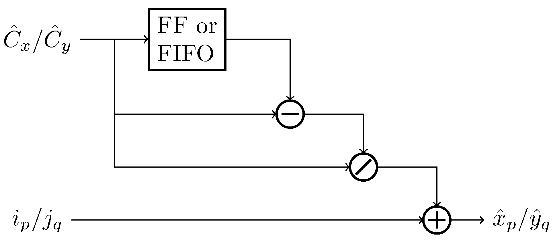
The implementation of the sub-pixel interpolation in the
x and
y directions according to Equations (5) and (6) is shown in
Figure 5. To interpret the sub-pixel shift
, the centroid estimation from the previous pixel is required, which can be buffered by a FF register. For the sub-pixel shift in the
y direction, however, the pixel in the previous row is needed, which means the whole row of centroids value in
y direction needed to be buffered in a FIFO with depth that is the same as the column number.
3.2. Segmentation Module
The stream-based CoG algorithm itself is able to determine multiple spots presented in a sub-aperture if the filter size is not so large as to cover all the spots. Recall that the filter size is matched to the spot size, not the sub-aperture size Equation (3). How to use these extra centroids to achieve a better local slope estimation (Z-tilt instead of G-tilt) or reconstruct wavefront from multiple sources is a simple sorting procedure is beyond the scope of this paper. Here, we try to render a traditional array of centroids corresponding to the lenslet array from the SCoG detected centroids through the Segmentation module using the following steps.
3.2.1. Centroid Sorting Module
It is assumed that all the detected centroids in one sub-aperture truly belong to this sub-aperture. In other words, there are no spots crossing lenslet boundaries due to strong aberration. In order to associate a detected centroid to its sub-aperture, Equation (
7) was used to calculate the row and column index of the sub-aperture. When the number of pixels per lenslet window and integer of power is two, the division can be simplified to bit shifts.
3.2.2. Treatment of Multiple Centroids and Missing Centroid
As discussed in
Section 2.3, there are different ways to treat the scenarios where multiple centroids or no centroid is detected in some sub-apertures. For the current FPGA implementation, the average of all the centroids within a sub-aperture is used to represent an overall displacement for the multiple centroids situation. If a centroid is missing from a sub-aperture, then the centroid position from previous frame is inherited, which can trace back to an initial default reference centroid positions for each sub-aperture.
Once the centroids for the last sub-aperture in a row have been examined following by the slope calculation, the partial wavefront reconstruction can start immediately. The above segmentation steps can be represented by the pseudocode in Algorithm 1:
| Algorithm 1: Pseudocode for sorting–processing–reordering. |
Data: stream centroid Result: ordered centroid for each sub-aperture |
3.3. Slope Calculation Module
After the SCoG and Segmentation modules, there will be an averaged centroid for each sub-aperture similar to conventional CoG-based methods. The SLOPE module calculates local slopes of wavefront in each sub-aperture according to Equation (1). An initial reference grid is stored in this module, where the reference center is designed to be in the center of each sub-aperture. This module is also capable of updating the reference centroids grid by averaging a certain frames of centroids data. This is particularly useful when applying the wavefront sensing system to an imaging system where a flat wavefront is not accessible. Therefore, the reference grid must be calculated by averaging the centroids from a number of long exposure images.
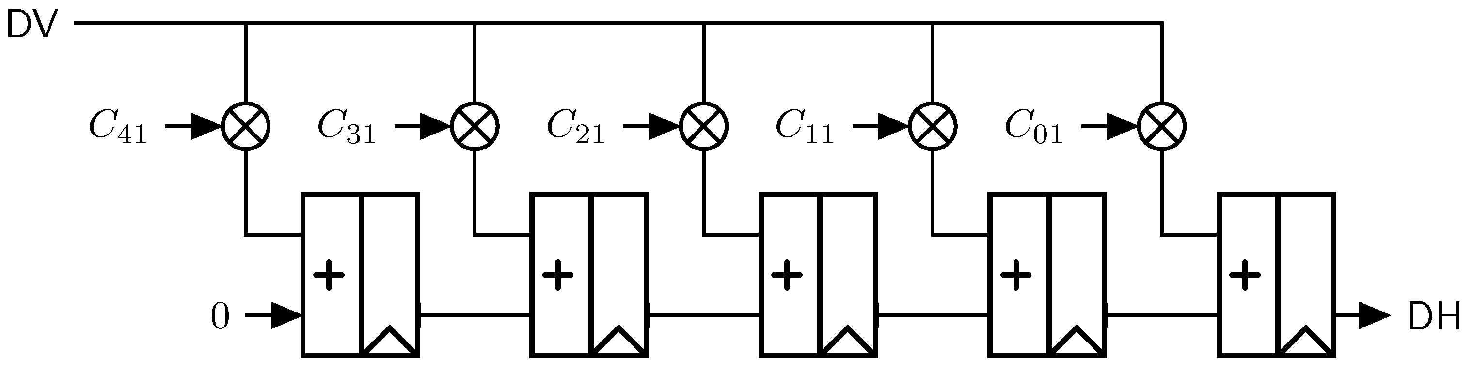
3.4. Wavefront Reconstruction Module
The wavefront reconstruction module essentially computes a matrix multiplication between the inverse matrix and the slope vectors according to Equation (
12). As the slopes for each sub-aperture are measured, they are multiplied by their corresponding matrix elements and accumulated with previous multiplication. The calibration matrix
E is determined once the geometric configurations is fixed and therefore can be calculated in advance. When the slopes of all the sub-apertures in the same row are measured and multiplied, the next section of the matrix corresponding to the slopes of next row of sub-apertures are loaded. The loading of new matrix elements is controlled by a finite state machine (FSM).
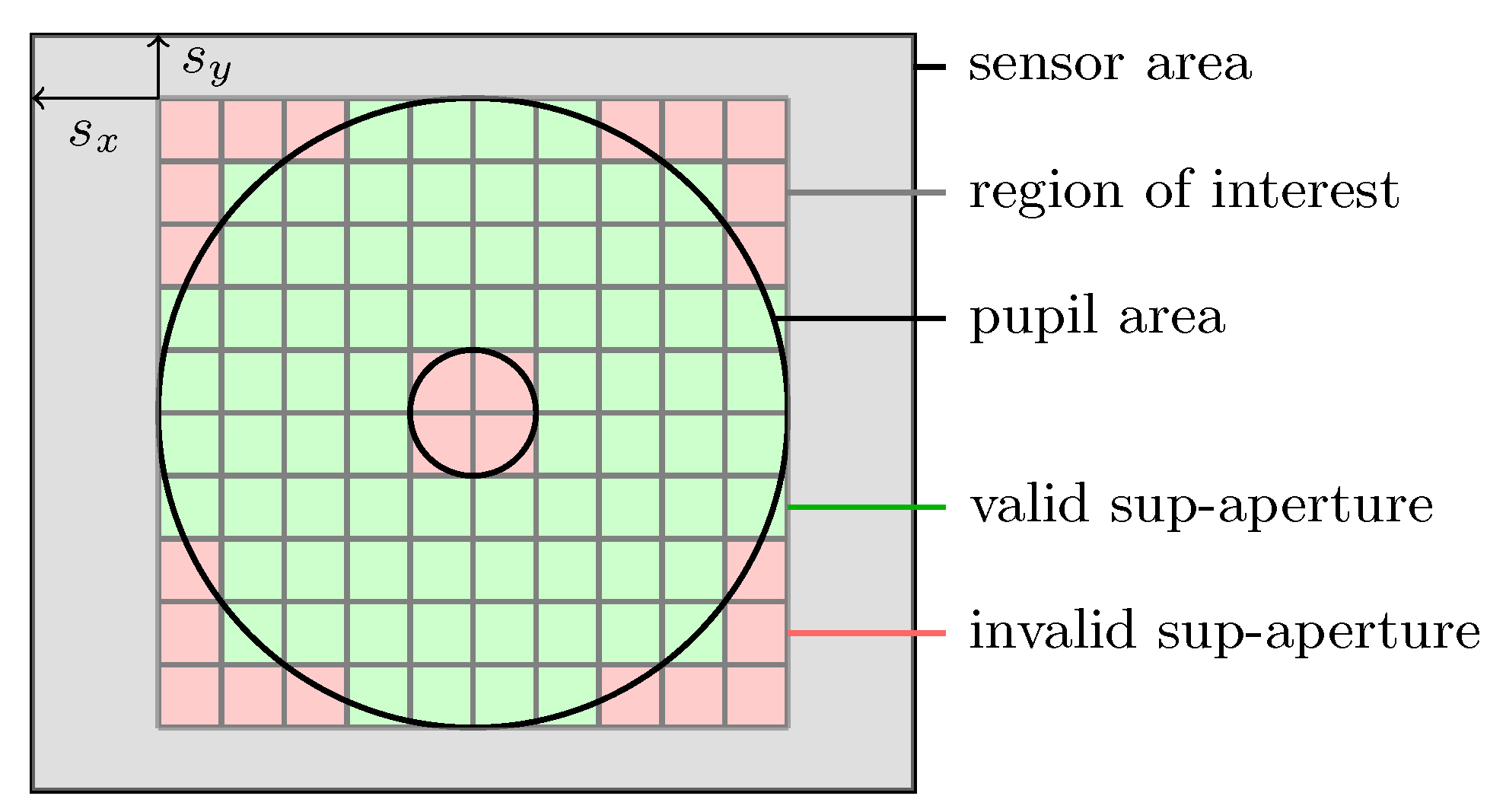
In
Figure 6, different areas related with the SHWFS are shown. The gray sensor area includes all the selected active imaging sensor pixels, on which the SCoG is operated. The resulted detected centroids from the SCoG module are represented on this sensor coordinate system. Since most AO systems have either a circular or annular Pupil, a square ROI was chosen to include the Pupil. After removing the ROI origin offset
from the centroids calculated by the SCoG module, the local centroids were obtained on the ROI coordinate system. Following that, the segmentation module can sort the centroids to their associated sub-apertures, followed by the slope module to obtain the average slope on individual sub-apertures. For the wavefront reconstruction, only slopes on those valid sub-apertures (green) were used. A binary sub-aperture mask indicating the validness of an sub-aperture was used to decide whether to accumulate matrix multiplication result to the partial wavefront reconstruction in the RECON module.
5. Discussion
In this paper, we have presented a complete hardware implementation of Shack–Hartmann wavefront sensor in a modular design. The spots displacement was measured using the previously reported Stream-based CoG algorithm, which reduces the centroid estimation error when the signal is cut by the sub-aperture boundary and noise-induced error by using a spot-matched floating CoG window. The slope calculation and wavefront reconstruction using a least-square fit method starts immediately as long as the required sub-aperture measurements are ready. The result is a very low-latency and real-time wavefront sensing system with superior performance to conventional CoG-based SHWFS facilitated by the parallelism power from FPGA devices.
The FPGA implementation of Stream-based Center-of-Gravity algorithm can be modified without much effort to adapt other filter-like algorithms, for example, the cross-correlation for determining image shifts under extended sources proposed by Poyneer [
6]. The First Fourier coefficient (1FC) algorithm [
38] examines the phase symmetry in the Fourier domain to evaluate the spot shifts. Both the CCF and 1FC algorithms can be modified to their streamed version with minimal effort based on the implementation presented in this work.
The current treatment of multiple centroids identified in one sub-aperture is to average them, which can be further improved by other algorithm events to increase the dynamic range such as [
36]. Future work also includes testing the proposed SHWFS implementation with the on-board image sensor in laboratory optics systems and eventually including the wavefront correction component, such as a deformable mirror, to realize a closed-loop AO system.


