Multi-Scale Cost Attention and Adaptive Fusion Stereo Matching Network

Abstract

At present, compared to 3D convolution, 2D convolution is less computationally expensive and faster in stereo matching methods based on convolution. However, compared to the initial cost volume generated by calculation using a 3D convolution method, the initial cost volume generated by 2D convolution in the relevant layer lacks rich information, resulting in the area affected by illumination in the disparity map having a lower robustness and thus affecting its accuracy. Therefore, to address the lack of rich cost volume information in the 2D convolution method, this paper proposes a multi-scale adaptive cost attention and adaptive fusion stereo matching network (MCAFNet) based on AANet+. Firstly, the extracted features are used for initial cost calculation, and the cost volume is input into the multi-scale adaptive cost attention module to generate attention weight, which is then combined with the initial cost volume to suppress irrelevant information and enrich the cost volume. Secondly, the cost aggregation part of the model is improved. A multi-scale adaptive fusion module is added to improve the fusion efficiency of cross-scale cost aggregation. In the Scene Flow dataset, the EPE is reduced to 0.66. The error matching rates in the KITTI2012 and KITTI2015 datasets are 1.60% and 2.22%, respectively.

1. Introduction

Computer vision is widely used in autopilot systems, unmanned aerial vehicles, intelligent manufacturing, augmented reality and other fields. In environments where human work is limited, computer vision can help with recognition and detection. As a type of computer vision technology, binocular vision uses binocular cameras to estimate depth based on stereo matching, and then obtains the three-dimensional information of the surrounding environment through the obtained depth information. It has high accuracy, a low cost and a small size and is suitable for complex environments. Binocular vision can be flexibly applied to intelligent robots, unmanned aerial vehicles and other equipment.

In recent years, compared to traditional methods, binocular stereo matching methods based on deep learning have seen great improvements in accuracy and speed. Among these methods, the single-scale method constructs a single cost volume based on the characteristics of a single-resolution image. This method processes a single cost volume and requires the use of 3D convolution in convolutional neural networks to improve its accuracy. However, the use of 3D convolution will increase the number of parameters in the model, resulting in reduced model speed. However, multi-scale methods, which fuse or process the images or cost volumes of different resolutions, can not only provide rich feature information for matching pixel points, but also be used in cost aggregation to improve the efficiency of matching costs. The multi-scale method combined with 2D convolution can obtain multi-scale information and aggregate the matching costs of multiple scales, achieving better results. Moreover, 2D convolution requires fewer parameters and has a small impact on model speed. However, using multi-scale methods to improve the robustness of the edges of objects and areas affected by illumination in real scenes, thus helping to better identify objects in subsequent 3D reconstruction tasks, remains a difficult problem to be solved by multi-scale methods. Therefore, investigations into multi-scale binocular stereo matching methods based on convolutional neural networks have high research value and significance. The research content and contributions of this article are as follows:

(1) Improvements have been made to the multi-scale model AANet+ [1], and experiments have been conducted on Scene Flow datasets and other real scene datasets. The experimental results show that the proposed model significantly improves the disparity in robustness compared to the benchmark model.

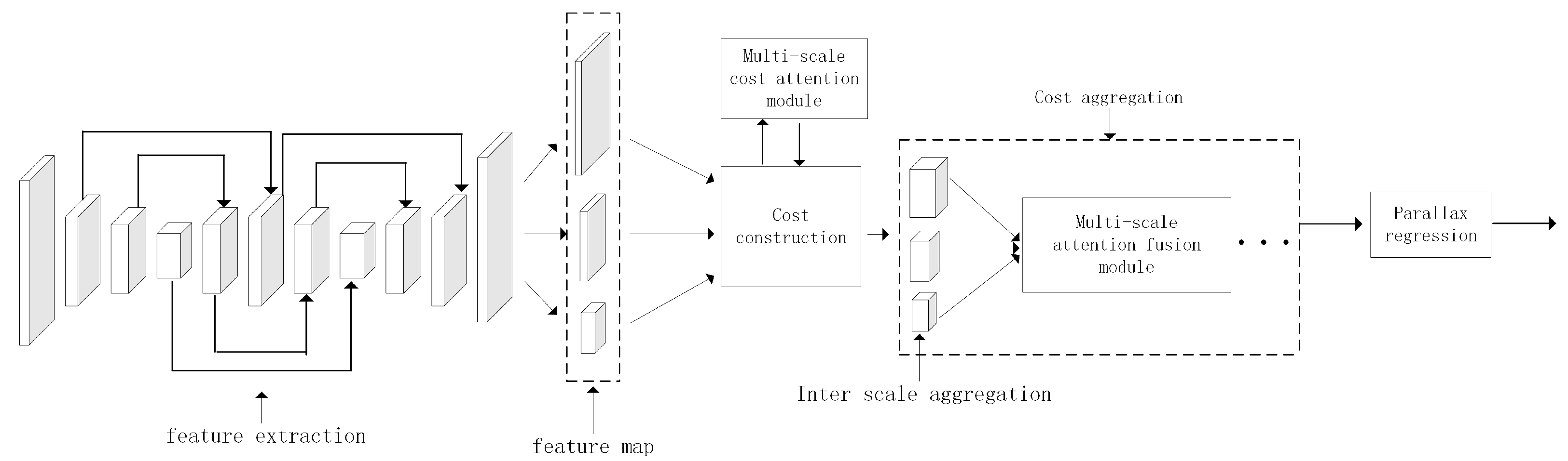
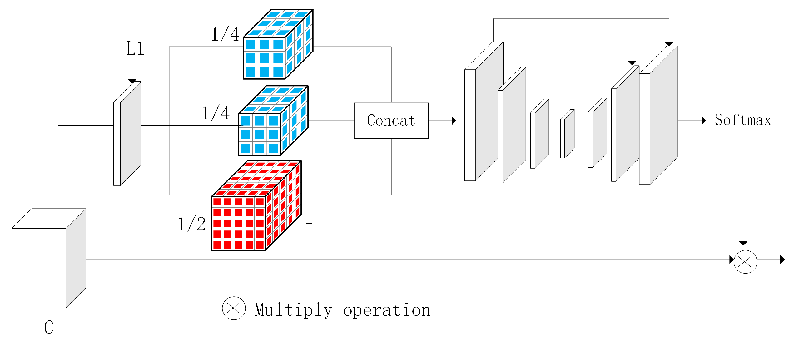
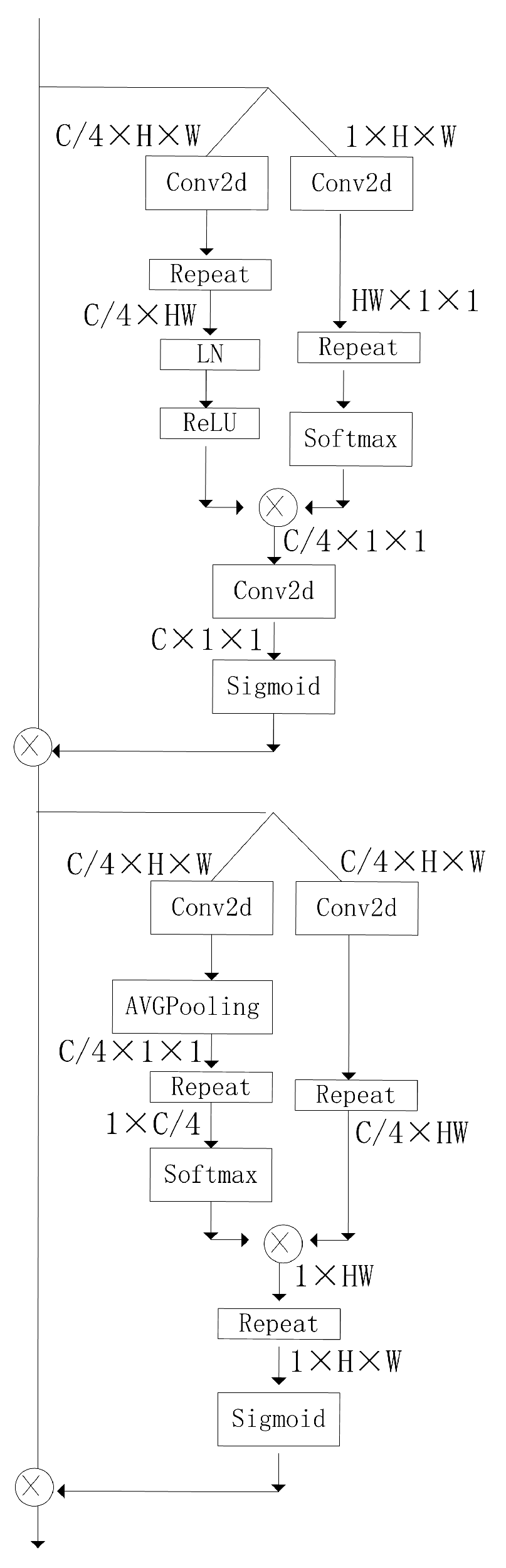
(2) Addressing the problem of low prediction disparity robustness in areas affected by light in real scenes in multi-scale stereo matching methods, a multi-scale cost attention module is added to suppress the redundant information and focus on areas affected by light.

(3) Addressing the problem of information loss caused by cross-scale fusion in multi-scale stereo-matching methods, an adaptive fusion structure is designed that utilizes a polarization self-attention mechanism to generate attention and fuse the attention with cost volumes to reduce information loss.

Based on the above, the research motivation in this article is mainly to reduce disparity errors in areas affected by light in disparity maps, and make contributions to subsequent 3D reconstruction tasks.

2. Related Works

Stereo-matching methods based on deep learning can be divided into single-scale stereo matching methods and multi-scale stereo matching methods according to the processing methods for different resolution cost volumes. Stereo matching based on multi-scale methods has been proven to improve the robustness of weakly or non-textured regions in disparity images. Inspired by traditional multi-scale stereo matching, Zhu et al. combined multi-scale methods with 3D convolution to obtain multi-scale features through multi-scale feature extraction and used cross-space pyramids to aggregate context information, improving the accuracy of multi-scale methods [2]. Inspired by image segmentation algorithms, Alex et al. proposed GC-Net [3], which uses a concatenation method to aggregate feature images obtained from feature extraction, concatenates left and right feature images to obtain cost volumes and uses a multi-scale method to aggregate cost volumes using 3D convolution to improve the accuracy of disparity maps. In order to effectively fuse multi-scale context information, Wu et al. proposed SSPCV-Net [4], which uses a recursive method to upsample low-resolution cost volumes, utilizes a 3D aggregation module to extract the multi-level features of cost volumes, gradually completes the fusion of multi-scale cost volumes and finally obtains a more accurate disparity map through disparity regression.

Shen et al. proposed that in the downsampling stage of the cost volume aggregation module, the cost volumes of different scales are directly fused, reducing the number of 3D convolutions used and preserving the disparity information for the cost volumes of different scales [5]. However, this method fails to adjust the disparity search range in a timely manner, and the generalization ability of the model needs to be improved. For this reason, Shen et al. proposed CFNet [6], which uses a multi-scale cost volume fusion method to fuse the cost volumes of different scales as initial cost volumes, obtaining an initial disparity map and then using a cascade method to adjust the disparity search range for uncertainties in the initial disparity map. The resolution of the disparity map is thus gradually improved and refined. This method effectively integrates multi-scale information and improves the generalization ability of the model.

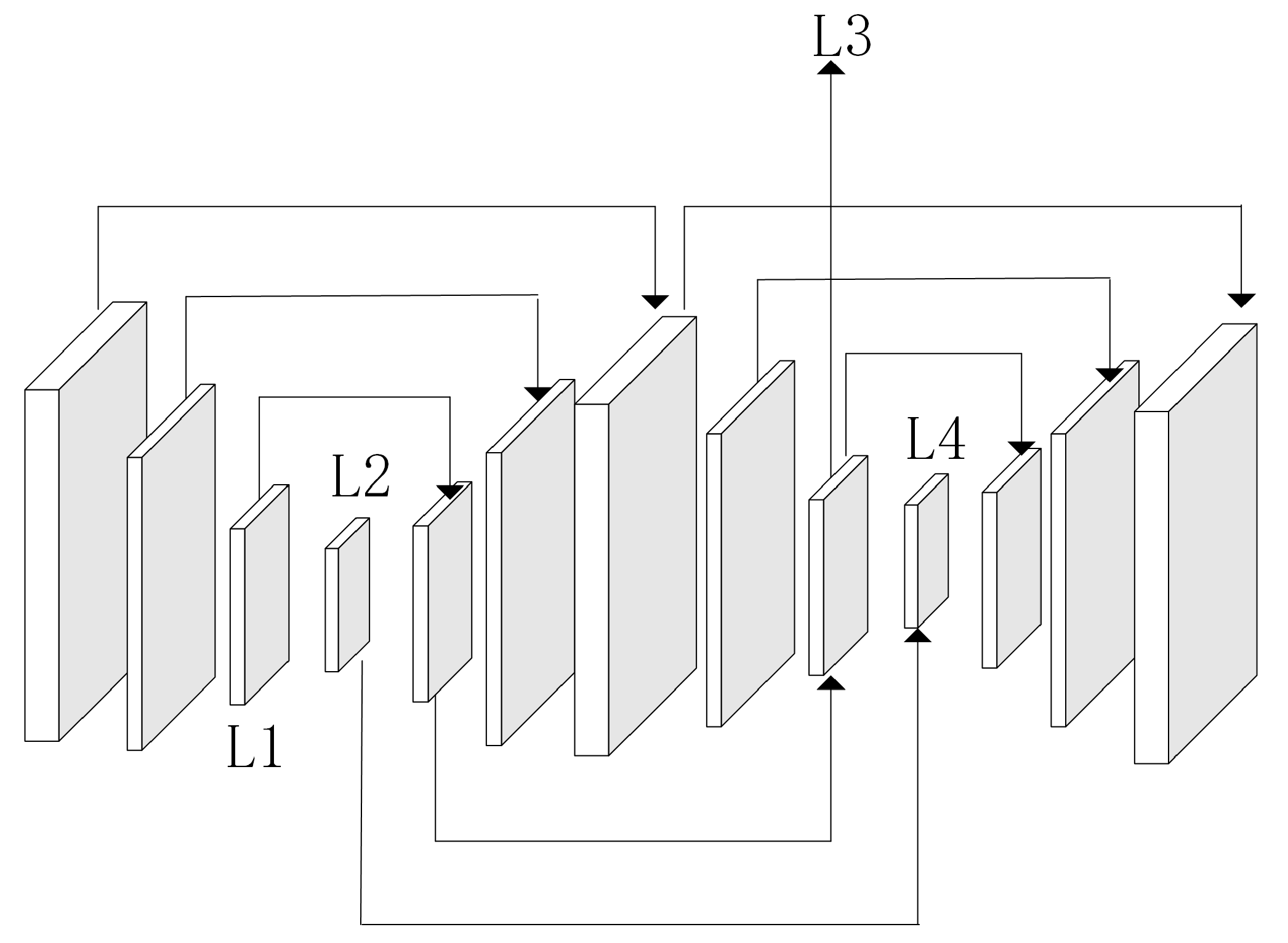
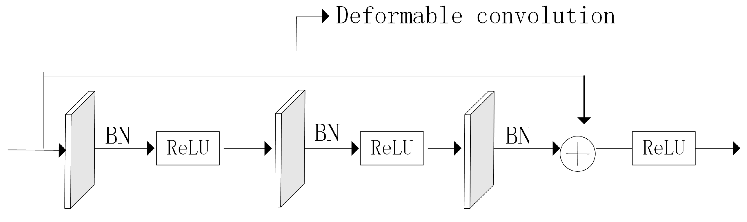
When the above multi-scale method is used in combination with 3D convolution, the model’s speed is slow due to the large number of parameters. In order to improve the prediction effect of the multi-scale method in weak and non-textured regions and to improve the speed of the model, Xu et al. proposed AANet [1], in which 2D convolution is used to establish a stereo matching network, and a multi-scale method is used to aggregate cost volumes. Deformable convolution is added to the network to achieve an adaptive effect on the model. Two cost-aggregation modules are proposed: cross-scale cost aggregation and intra-scale cost aggregation. This method balances the speed and accuracy of the model well. Li [7] and Jia [8] proposed two model structures, respectively. Their common feature is the use of an hourglass structure composed of 2D convolutions to aggregate multi-scale cost volumes, thereby reducing computational complexity and balancing the accuracy and speed of the model. Syed et al. [9] used multi-scale distortion features to estimate the disparity and minimize the disparity search range in the cost volume. They used a refined structure composed of 2D convolutions to process the disparity maps, reducing computational complexity while maintaining accuracy. Although the above network model achieves good balance between the accuracy and speed of stereo matching models, multi-scale information cannot be effectively fused, and its robustness is low in certain areas, such as object edge areas, foreground areas and occlusion areas.

In order to solve the problem of the high error match at the edges of multi-scale methods, Xue et al. used lightweight 2D and 3D multi-scale aggregation modules to aggregate low-resolution cost volumes and utilized multi-scale RGB image guidance for upsampling, improving the disparity robustness at the edges. However, the prediction effect on blocked areas and areas affected by lighting in the image is poor [10]. Yang et al. designed RDNet [11] to design a separate branch to learn edge information. Guided by edge information, RDNet improves the robustness of boundaries in disparity maps, and combines multi-scale methods to improve the accuracy of disparity maps. Jeon et al. [12] combined a multi-scale fusion structure with a cross-scale fusion function, using a staggered cascade method to combine the cost volumes of different scales. Finally, an adaptive cost volume loss function was used to estimate the cost. This method improves the disparity accuracy of the edges. Zhang et al. [13] proposed fusing low-level and high-level features to preserve image edge information, and designed a multi-scale cost aggregation module to extract rich global context information, reducing dependence on local information. Unlike HFMANet [13], Li et al. [14] designed a multi-channel group by group correlation method to construct cost volumes, and then used an adaptive cost aggregation method to regularize cost volumes from different scales through intermediate supervision. These two methods are helpful for disparity estimation in weak texture areas. Tao et al. [15] designed a stereo matching network with confidence perception unimodal cascaded and fused pyramids, using confidence graphs to construct a unimodal cost distribution to narrow the disparity search range. Then, a cross-scale interactive aggregation module is designed to fully utilize multi-scale information. This method improves the disparity robustness of occluded areas in disparity maps. Most of the methods mentioned above focus on the low robustness of edges and weak texture areas. However, in real scenes, objects are easily affected by light and become difficult to estimate disparity. Therefore, this paper proposes a multi-scale cost attention and adaptive fusion structure, which alleviates the problem of low disparity robustness in illuminated areas in real-scene datasets using multi-scale methods. In the Scene Flow dataset, the method proposed in this article further reduces endpoint errors and improves disparity robustness in non-textured regions and small structures.

3. Methods

Addressing the problem of the cost volume information in 2D convolution methods not being rich, a multi-scale cost attention stereo matching network is designed based on AANet+. The network structure is composed of feature extraction, cost construction, cost aggregation and disparity regression. Multi-scale feature fusion in AANet+ is adopted to improve the efficiency of feature extraction. In this paper, the cross-correlation layer is used to construct the cost volume, and a multi-scale cost attention module is proposed to generate the cost attention, multiply it with the initial cost, suppress redundant information and enhance the reliable information. For cost aggregation, this paper designs a multi-scale adaptive fusion module, which inputs the intra-scale cost into the multi-scale adaptive fusion module to improve the fusion efficiency. In the multi-scale attention module, the three scales of cost volume are input into the attention module, the generated attention is multiplied with the cost volume, and the results are fused to enhance the consistency of cost volume, reducing the inconsistencies in the cost characteristics caused by the direct fusion of different-scale cost volumes and improve the efficiency of cross-scale fusion. Finally, the soft argmin method is used for disparity regression. The structure is shown in Figure 1:

3.1. Feature Extraction and Multi-Scale Cost Attention

In AANet+, a cascade U-shaped network is used for feature extraction, and then three scales of convolution layers are used to output feature maps with 1/3, 1/6 and 1/12 resolutions, respectively. In order to improve the efficiency of feature extraction, deformable convolution is added. Unlike ordinary convolution, deformable convolution can add an offset to the sample points and adaptively sample the feature points to a specific location. The structure is shown in Figure 2.

In Figure 2, L1, L2, L3 and L4 are deformable convolution layers, and the features are fused by feature splicing, which can reduce the loss of feature information. There is a lack of improvement in the cost construction method in stereo matching networks based on 2D convolution. After feature extraction, most stereo matching networks use relevant layers similar to FlowNetC [16] to structure the cost. This method uses a matrix product, which is fast, but its accuracy is lower than that of the grouping cost volume method in GwcNet [17]. Therefore, multi-scale adaptive cost attention is added to the cost calculation to improve the accuracy of the initial cost volume. In contrast to ACVNet [18], this module adopts 2D convolution. After adaptive selection by deformable convolution [19], the cost volume is input into the pyramid structure with an attention mechanism to refine multi-scale information, further enrich the cost volume, improve the attention accuracy of the cost and make up the gap between 2D convolution and 3D convolution. Taking the cost volume with 1/3 resolution as an example, the multi-scale adaptive cost attention module is shown in Figure 3.

Attention weight is used to filter the initial cost volume, allowing the model to pay attention to useful information and reduce unnecessary information. The method of calculating the cost volume in the cross-correlation layer is realized by calculating the similarity between pixels, which becomes unreliable due to the lack of sufficient matching information, resulting in a disparity map with low accuracy in ill-posed areas, such as dark areas. Therefore, attention weights are generated by extracting geometric information from the correlation between a pair of stereoscopic images. Figure 3 illustrates the idea of multi-scale adaptive cost attention. Multi-scale cost attention can be divided into three parts. First, the left and right feature maps are obtained from the feature extraction module, and the cost volume is calculated using the correlation method. Then, after initial adaptive selection, the cost volume is grouped by channels, including two 1/4 channels and one 1/2 channel. For each pixel, dilated convolution is used to control the expansion rate to ensure that the range of the receptive field corresponds to the feature map, and to improve the accuracy of the pixel similarity calculation. Then, the grouped cost volume is spliced into the given number of channels before grouping, and the spliced cost volume is optimized through a pyramid-like structure. In pyramid structures, in order not to lose the cost volume information, a channel attention mechanism [20] is added to improve the accuracy of the adaptive cost volume attention. Finally, in order to obtain accurate cost attention, the softmax function is used to obtain the weight of the cost attention and multiply it by the initial cost volume to obtain the refined initial cost volume. The formula is shown in Formula (1):

$$C(d,h,w)=\frac{1}{N}〈F_l^s(h,w),F_r^s(h,w-d)〉\otimes \theta$$

(1)

where $〈F_l^s(h,w),F_r^s(h,w-d)〉$ represents the inner product of feature vectors, n represents the number of channels for extracting features, $C(d,h,w)$ represents the calculated cost, ⊗ represents that attention is multiplied by the cost of the initial construction and $\theta$ represents the generated cost attention.

3.2. Multi-Scale Attention Fusion Module

3.2.1. Cost Aggregation in AANet+

In AANet+ [1], there are two methods of cost aggregation: intra-scale cost aggregation and cross-scale cost aggregation. Intra-scale cost aggregation is completed by deformable convolution [19,21], and the sampling points are adaptively aggregated to similar disparity positions through deformable convolution to solve the problem of disparity discontinuity. The formula of intra-scale aggregation is shown in Formula (2):

$$C^I(d,p)=\sum _{k=1}^{K^2}{W}_k\ast C(d,P+P_k+\Delta P_k)\ast m_k$$

(2)

where $C^I(d,p)$ represents the aggregated cost of disparity d at pixel p, k represents the number of sampling points, $W_k$ represents the aggregation weight and $P_k$ represents the fixed offset based on the window cost aggregation method. In order to achieve efficient adaptive aggregation, $\Delta P_k$ is added to represent the additional offset that can be learned, so as to obtain ideal results from edges and thin structures. $M_k$ denotes the position weight, which is used to control the mutual influence of positions between pixels, thus strengthening adaptive aggregation. Intra-scale cost aggregation adopts a residual structure, where the middle convolution layer is a deformable convolution and the rest are ordinary convolutions, as shown in Figure 4.

After intra-scale aggregation, AANet+ designs a similar full-connection method to aggregate the cost of three different scales of intra-scale aggregation following the idea of aggregating the cost of different scales in the traditional cross-scale aggregation algorithm [22]. This solves the problem of poor disparity robustness in weakly or non-textured regions. As shown in Formula (3):

$$C^S=\sum _{k=1}^S{f}_k\left(C^{Ik}\right)$$

(3)

where $C^S$ is the cost after cross-scale aggregation, $C^{Ik}$ is the cost volume after intra-scale aggregation and $f_k$ is the general function; that is, when k = s, the cost is multiplied by a fixed value; when k < s, the cost volume is downsampled 2$s-k$ times; and when k > s, the cost volume is first upsampled to the same resolution and then uses a 1 × 1 conv alignment channel. However, the cross-scale aggregation method simply adds three different scales of cost entities. The features of different scales may be inconsistent in scale and semantics. Direct addition will easily result in the loss of cost information, which will have a certain impact on the quality of the disparity map.

3.2.2. Adaptive Fusion Module

In view of the problems of cross-scale aggregation in AANet+ [1], a multi-scale adaptive fusion module is designed to replace the simple addition structure in cross-scale aggregation. The attention module uses polarized self-attention to enhance the accuracy of multi-scale aggregation. The adaptive fusion module formula is shown in Formula (4):

$$\widehat{C}=L\left(C\right)\otimes C_K+C_I\otimes L\left(C\right)$$

(4)

where $\hat{C}$ is the cost after aggregation, C is the initial fusion cost and $C_K$ and $C_I$ are the costs of different scales after cost aggregation within the scale, where $C_I$ is the cost multiplied by a fixed value when k = s and $L\left(C\right)$ is the polarizing self-attention module. Taking scale H/12 as an example, the multi-scale adaptive fusion structure is shown in Figure 5.

In contrast to the fusion of attention features (AFF) [23], for the three-input scale cost volumes, C1 and C2 are the input into the attention module, and the weight is generated after the input passes through the attention module. The generated attention mechanism is multiplied by C1 and C2 separately, and then C1 and C2 are fused. Finally, the above operation is repeated using the fused cost and C3. The cost volume is multiplied with the corresponding weight generated, and attention is paid to important information and the cost volume is enriched, thus reducing the information lost by simply fusing the cost. The added attention module is shown in Figure 6.

Most of the attention mechanisms introduced in stereo matching tasks are channel attention mechanisms, such as in SENet [24], or the combination of channel attention mechanisms and spatial attention mechanisms, such as in CBAM [20]. Channel attention can assign the same weight to different spatial positions to improve the accuracy of stereo matching tasks. In order to improve the fusion efficiency and improve the accuracy of the disparity map from the pixel level, the attention mechanism combining the pixel-level channel self-attention and spatial self-attention [25] is adopted. Firstly, the number of channels is changed to 1 and C/4 through the convolutional layer. Then, the cost volume matrix is reorganized through two tensor shaping operators. The cost volume with one channel is normalized using softmax and multiplied by the cost volume in the orthogonal direction. Finally, the channel is adjusted through convolution, and channel self-attention is generated using the sigmoid function. The formula for channel self-attention in the polarized attention mechanism is as follows:

$$C_{ch}=\sigma \left[F\left((R\left(F\left(C\right)\right)\times Softmax\left(R\left(F\left(C\right)\right)\right))\right)\right]$$

(5)

where C represents the cost volume, F represents a convolution layer, R represents the tensor reshape operator, $\sigma$ represents the sigmoid and $C_{ch}$ represents the generated channel cost attention.

In spatial self-attention, the fusion cost volume is firstly folded into 1 × 1 resolution features through adaptive average pooling, generating pixel-level spatial attention through softmax, and H × W high-resolution features are multiplied. Finally, the sigmoid function is used for mapping to generate the attention mechanism output. The formula for spatial self-attention in the polarized attention mechanism is as follows:

$$C_{sq}=\sigma \left[R\left((Softmax\left(R\left(\left(AVG\left(F\left(C\right)\right)\right)\right)\right)\times \left(R\left(F\left(C\right)\right)\right))\right)\right]$$

(6)

where $C_{sq}$ represents the generated spatial cost attention and AVG represents average pooling. The polarization attention mechanism of pixel-level regression is different from CBAM in that the polarization attention uses softmax and sigmoid in both channel and space to inject pixel-level attention into features, so as to pay full attention to the cost information and improve the fusion efficiency.

3.3. Disparity Regression

For each pixel, the soft argmin method [3] is used for disparity regression. The disparity regression method is differentiable and can return sub-pixel precision disparity, which is helpful to improve the disparity regression accuracy, so it is applied to the proposed model. The formula is as follows:

$$d=\sum _{d=0}^{D_{max-1}}d\ast \sigma \left(C_d\right)$$

(7)

where $D_{max-1}$ represents the maximum disparity, $\sigma$ represents the sigmoid function, $C_d$ represents the cost volume obtained through cost aggregation and upsampling and $\sigma \left(C_d\right)$ can be expressed as the probability of disparity.

3.4. Loss Function

Because the data in the Scene Flow dataset [26] have a large number of truth labels, the smoothL₁ loss function is used to train the Scene Flow dataset:

$$L=\frac{1}{N}\ast \sum _{i=1}^{N}smooth{L}_1(d_{pred},d_{gt})$$

(8)

where the smoothL₁ function is:

$$smooth{L}_1(d_{pred},d_{gt})=\left\{\begin{array}{cc}0.5{(d_{pred}-d_{gt})}^2,\hfill & if\left|d_{pred}-d_{gt}\right|<1\hfill \\ \left|d_{prd}-d_{gt}\right|-0.5,\hfill & otherwise\hfill \end{array}\right.$$

(9)

where N represents the number of labeled pixels, $d_{pred}$ represents the predicted disparity and $d_{gt}$ represents the true value of disparity. Because the KITTI [27,28] dataset lacks the truth label, the KITTI dataset trained by the existing model with good effect is used as the false label [1]. Therefore, the loss function under the KITTI dataset is:

$$L=\sum _{i=1}^{N}smooth{L}_1(D_{pred}^i,D_{pseudo})$$

(10)

where p represents the pixel, and $D_{pseudo}$ represents a false label true value.

4. Experiments and Result

4.1. Datasets

Middlebury: The Middlebury [29] dataset consists of four datasets, including data from 2001, 2003, 2005, 2006, 2014 and 2021. The latest dataset was proposed by Literature 66 and was captured by Middlebury College using a mobile device on a robotic arm. The latest dataset can be divided into 3000 × 2000 resolution, 1500 × 1000 resolution and 750 × 500 resolution.

Scene Flow: The Scene Flow dataset is a 3D composite dataset, subdivided into the FlyingThings3D dataset, Driving dataset and Monkaa dataset. The Scene Flow dataset has a total of over 30,000 pairs of training images, with a pixel size of 540 × 960, which contain abundant training samples and dense disparity maps. It has become a mainstream pre-training dataset in recent years.

KITTI: The KITTI dataset is a real road scene dataset collected by an international team through mobile vehicles using laser radar to obtain image depth information and convert it into disparity. Therefore, the disparity value obtained is relatively accurate. The dataset contains a total of over 300 pairs of images, including KITTI2012 and KITTI2015. The KITTI2012 and KITTI2015 datasets use 154 image pairs and 160 image pairs as training sets, respectively.

4.2. Experimental Setting

This experiment uses the Python framework, and the construction of the network environment and the training process in the experiment are run on the server configured as an NVIDIA Tesla T4 GPU. In this paper, four datasets are used for the experiment, namely Scene Flow, Middlebury, KITTI2015 and KITTI2012. For the Scene Flow dataset, this experiment was inspired by ACVNet and trained three times. First, the multi-scale adaptive cost attention was trained, and then the weight of the attention obtained from the training was frozen for the second training. The second training combined the multi-scale adaptive attention structure with the backbone network, and the obtained training parameters were saved. Finally, the weight obtained from the second training was trained with the final network and the final stereo matching network was obtained. The purpose of the three training sessions was to obtain a multi-scale cost attention with high accuracy and keep it intact, so that the model can improve its accuracy on ill-posed areas in the disparity map after applying the multi-scale cost attention, such as the areas affected by light and small areas.

In the Scene Flow dataset, the image is randomly cut to a 288 × 576 resolution, and a verification set size of 540 × 960 resolution is set with an initial learning rate of 0.001 and an epoch of 64 and optimized using the Adam optimizer $({\beta }_1=0.9,{\beta }_2=0.999)$. After the 20th epoch, the learning rate is reduced to once every 10 epochs. For the KITTI2012 dataset, this experiment uses the pre-training model generated by the Scene Flow dataset for training and fine-tunes the model parameters. However, for the KITTI2015 and KITTI2012 datasets, the same strategy as that in [1] is adopted for disparity prediction; that is, the true value of disparity is used as supervision to improve the accuracy of the model in this dataset. The maximum disparity is set to 192. In this paper, the model generalization experiment is carried out in the Middlebury dataset. The pre-training model in the Scene Flow dataset is used to test directly on the Middlebury dataset. The resolution of the image is one-quarter of the resolution.

4.3. Experimental Results Analysis

Ablation Study

In order to verify the effectiveness of the network modules mentioned in this paper, an ablation experiment was carried out on the Scene Flow dataset. The models’ designs were compared, and four schemes were used to evaluate the proposed model.

The first scheme is the training reference network, and the resulting endpoint error is 0.831. The percentage of difference outlier (D1) is 0.340, the proportion of pixels with a prediction error greater than 1PX is 0.0880, the proportion of pixels with a prediction error greater than 2PX is 0.0534 and the proportion of pixels with a prediction error greater than 3PX is 0.0405.

The second scheme is to train the network with multi-scale cost attention, and the resulting endpoint error is 0.776. The percentage of difference outlier (D1) is 0.304, the proportion of pixels with a prediction error greater than 1PX is 0.0918, the proportion of pixels with a prediction error greater than 2PX is 0.0509 and the proportion of pixels with a prediction error greater than 3PX is 0.0368. When the multi-scale cost attention is added separately, the key information in the cost volume is focused, and the redundant information is reduced, so all errors are greatly reduced.

The third scheme is to train the network model with multi-scale adaptive fusion, and the resulting endpoint error is 0.783. The percentage of a difference outlier (D1) is 0.332, the proportion of pixels with a prediction error greater than 1PX is 0.0908, the proportion of pixels with a prediction error greater than 2PX is 0.0516 and the proportion of pixels with a prediction error greater than 3PX is 0.0386. When the adaptive fusion module is added separately, it reduces the loss of price information in the cross-scale aggregation of the network model, so the error decreases.

The fourth scheme is the network proposed in this chapter, and the resulting endpoint error is 0.664. The percentage of difference outlier (D1) is 0.227, the proportion of pixels with a prediction error greater than 1PX is 0.0638, the proportion of pixels with a prediction error greater than 2PX is 0.0369 and the proportion of pixels with a prediction error greater than 3PX is 0.0271.

The results of the whole ablation experiment are shown in

Table 1. Ablation experiment of network models.

	EPE	D1(%)	1PX(%)	2PX(%)	3PX(%)
Baseline	0.831	3.40	8.80	5.34	4.05
Multi-scale cost attention	0.776	3.04	9.18	5.09	3.68
Multi-scale adaptive fusion	0.783	3.32	9.08	5.16	3.86
MCAFNet	0.664	2.27	6.38	3.69	2.71

, where D1 represents the pixel proportion of the first frame image prediction error, and 1PX, 2PX and 3PX represent the errors of the pixel points. The values of these four indicators are in the form of percentages. From the table, we can see that the network proposed in this paper has the lowest error in the ablation experiment.

4.4. Generalization Study

The visualization results are as follows:

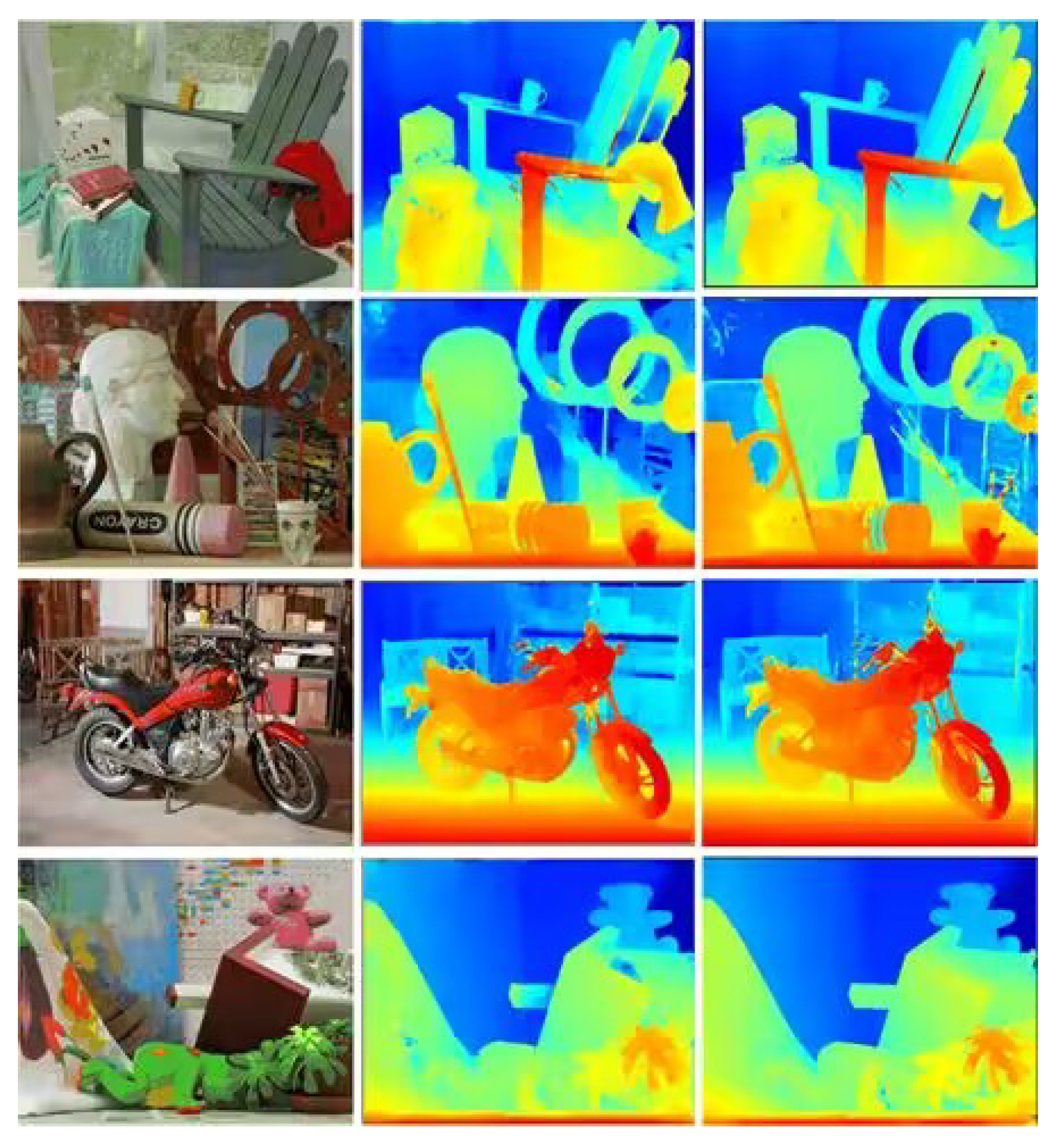
In Figure 7, the first column is the original image, the second column is the predicted disparity map for AANet+ and the third column is the predicted disparity map for MCAFNet. As can be seen from the figure, MCAFNet has a low mismatch rate in non-textured areas such as chairs and human faces.

Addressing the generalization performance of the proposed model, a generalization experiment is carried out in the Middlebury [29] dataset. For the generalization experiment, both the model in this paper and the benchmark network model adopt the pre-training model of the Scene Flow dataset, and the comparison index is the percentage of pixels with errors larger than 2 pixels (Bad2.0), that is, the error ratio is under 2 pixels. As shown in

Table 2. The generalization experiment of our network and benchmark model AANet+.

Network	Bad2.0	Time (s)
AANet+ [1]	50.7	0.16
MCAFNet	40.3	0.21

, although the speed difference between the proposed network and the benchmark network model AANet+ is 0.05 s, the error matching rate of MCAFNet is 20% lower than AANet+.

4.5. Comparative Experiment

4.5.1. Comparative Experiments on the Scene Flow Dataset

For the Scene Flow dataset,

Table 3. Comparison of indicators of different networks on the Scene Flow dataset.

Network	EPE	Time (s)
AANet [1]	0.88	0.06
PSMNet [30]	1.09	0.41
GCNet [3]	2.51	0.90
AANet+ [1]	0.83	0.16
MCAFNet	0.66	0.21

reflects the quantitative evaluation results of this network and GC-Net, PSM-Net, AANet and AANet+. The evaluation indicators used in this paper are the end point error (EPE) and time. For the Scene Flow dataset, we can see from Table 3 that the MCAFNet method proposed in this paper has better accuracy. Compared with AANet, the difference in speed of the network proposed in this paper is 0.15 s, and only 0.05 s compared with the reference network AANet+. Compared with other 3D convolution-based network models, namely PSM-Net and GC-Net, the speed of the network proposed in this paper is 48% and 76% higher, respectively. In terms of accuracy, the end point error of the network mentioned in this chapter is approximately 20% lower than that of AANet+. Compared with the PSNet and GCNet network models, the precision of the network proposed in this paper decreased by 39% and 73%, respectively.

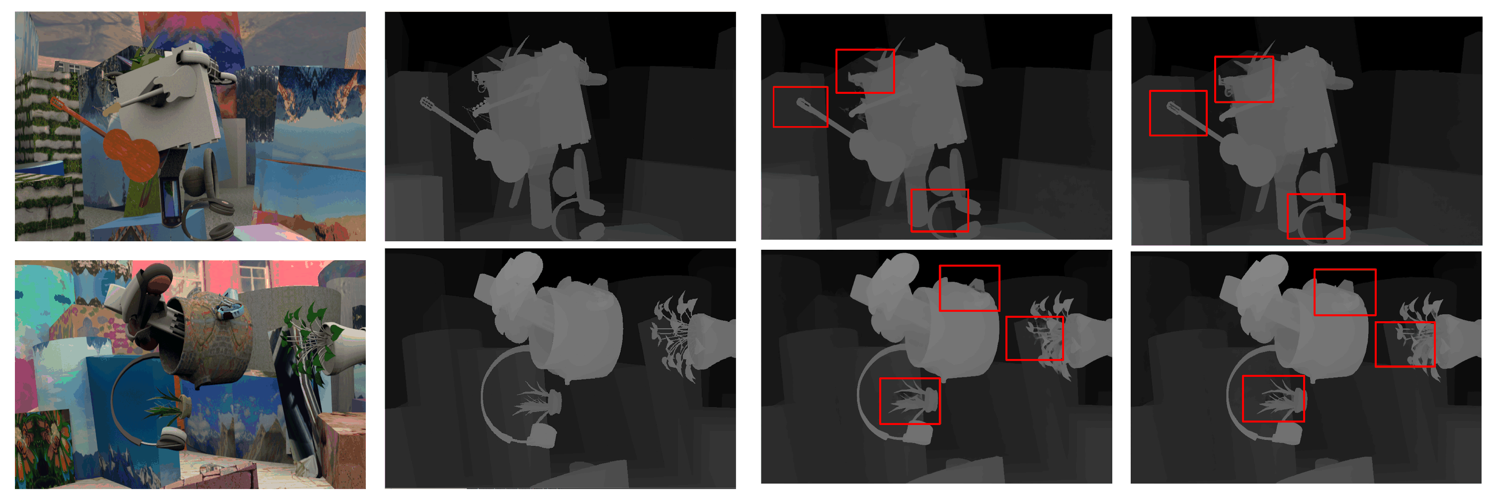
On the Scene Flow dataset, the proposed network is visually compared with the reference network model AANet+. The visual comparison results are shown in Figure 8. It can be seen from the red box in Figure 8 that, compared with AANet+, MCAFNet’s predicted disparity map is closer to the true disparity map. Compared with the reference network, it improves the accuracy in the case of a small speed difference.

4.5.2. Comparative Experiments on the KITTI2012 Dataset

In this paper, the evaluation indicators provided by the KITTI dataset are used for comparison. The comparison indicators of the KITTI 2012 dataset are the non-occluded area error (Noc) of 2PX(pixel), 3PX (pixel) and 5PX (pixel) and all area errors (All). It can be seen from

Table 4. Comparative experiment on the KITTI2012 dataset.

Network	2PX		3PX		5PX
	Noc(%)	All(%)	Noc(%)	All(%)	Noc(%)	All(%)
AANet [1]	2.90	3.60	1.91	2.42	1.20	1.53
ERSCNet	2.97	3.66	1.80	2.30	1.04	1.36
GCNet [3]	2.71	3.46	1.77	2.31	1.12	1.46
iResNet-i2 [32]	2.69	3.34	1.71	2.16	1.06	1.32
SegStereo [31]	2.66	3.19	1.68	2.03	1.00	1.21
MSDCNet [33]	2.71	3.37	1.63	2.09	0.98	1.26
AANet+ [1]	2.62	3.40	1.71	2.15	1.22	1.38
MCAFNet	2.40	3.05	1.60	2.08	1.02	1.34

that, compared with AANet+, the error of MCAFNet in the non-occluded area on the KITTI2012 dataset is significantly reduced. Under the evaluation indicators of 2, 3 and 5 pixels in all areas, the error of the network mentioned in this paper is reduced by 0.35, 0.07 and 0.04, respectively, which proves that the prediction of disparity of the network mentioned is more accurate than that of the reference network. Compared with GCNet and ERSCNet, MCAFNet has a good performance in error matching rate in the comparison results of 3 pixels and 5 pixels. At 3 pixels, the Noc mis-matching rate decreases by 9.6% and 11%, respectively. With the exception of SegStereo [31], iResNet-i2 [32] and MSDCNet [33], the network in this paper has the lowest Noc and All mismatch rates compared with the remaining network models.

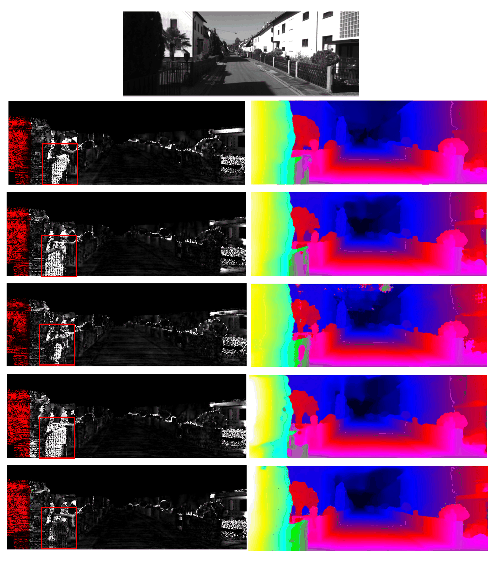
The comparison results of this model with AA-Net+ and iResNet-i2 on the KITTI2012 dataset are shown in Figure 9. The comparison results are provided by the KITTI dataset. In Figure 9, the first line is the original map, the second line is the iResNet-i2-predicted disparity map and the third line is the AANet+-predicted disparity map. The fourth line is the GCNet-predicted disparity map. The fifth line is the AANet-predicted disparity map. The sixth line is the prediction disparity map of the network proposed in this paper. It can be seen from the red box mark in the error map that, compared to other multi-scale methods, our proposed model can better predict disparity in the illuminated area.

4.5.3. Comparative Experiments on the KITTI2015 Dataset

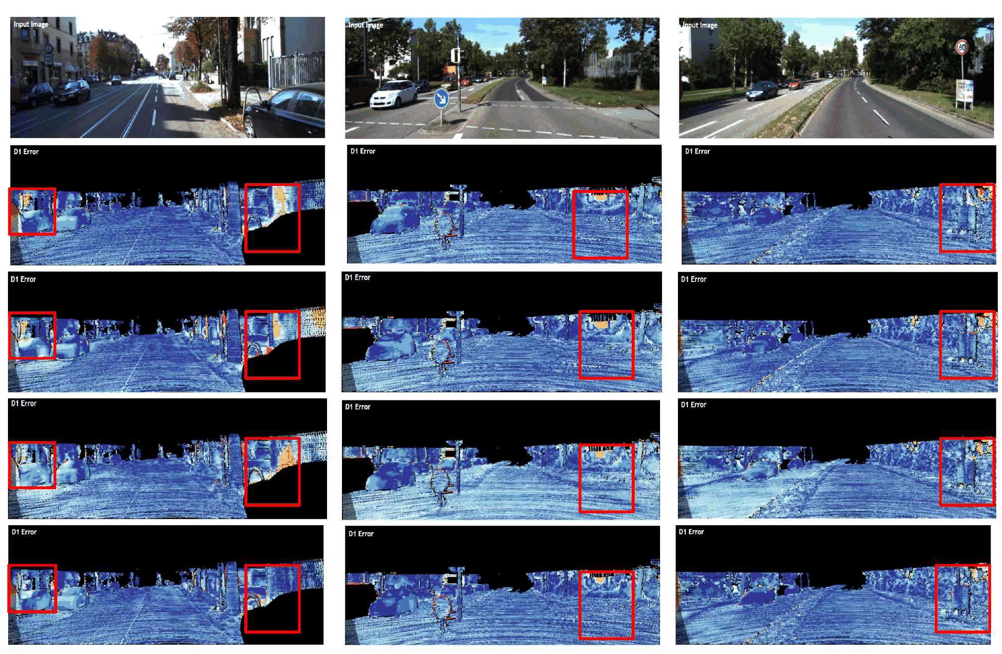
The comparison results of this model and AA-Net+ on the KITTI2015 dataset are shown in Figure 10. The comparison results are provided by the KITTI dataset. In Figure 10, the first line is the original map, the second is the predicted disparity map of AANet+. The third line is the error diagram of GCNet. The fourth line is the error map of AANet, and the fifth line is the error map of our proposed model network. From the red box mark in the figure, compared to other multi-scale methods, our proposed model can better predict disparity in the illuminated area.

The evaluation index provided by the KITTI2015 dataset is used for comparison. The comparison index of the KITTI2015 dataset is the proportion of predicted error pixels in the foreground area (D1 fg), background area (D1 bg) and all areas (D1 all) in the first frame of the image. It can be seen from

Table 5. Comparative experiment on the KITTI2015 dataset.

Network	Noc			All
	D1-fg(%)	D1-bg(%)	D1-All(%)	D1-fg(%)	D1-bg(%)	D1-All(%)
MADNet [36]	8.41	3.45	4.27	9.20	3.75	4.66
SMV [37]	8.82	3.28	4.20	9.32	3.45	4.43
Reversing-PSMNet [38]	8.33	2.97	3.86	8.70	3.13	4.06
DSMNet-synthetic [39]	6.19	2.84	3.34	6.72	3.11	3.71
ACOSF [40]	7.23	2.58	3.35	7.56	2.79	3.58
BGNet [34]	4.34	1.91	2.31	4.74	2.01	2.51
AdaStereo [41]	5.06	2.39	2.83	5.55	2.59	3.08
PVStereo [42]	5.73	2.09	2.69	6.50	2.29	2.99
SegStereo [31]	3.70	1.76	2.08	4.07	1.88	2.25
Separable Convs [43]	3.77	2.68	2.03	4.36	1.90	2.31
FADNet [35]	2.61	2.35	2.39	3.10	2.50	2.60
PSMNet [30]	4.31	1.71	2.14	4.62	1.86	2.32
AANet+ [1]	4.16	1.89	2.11	4.68	1.96	2.28
MCAFNet	3.92	1.61	1.99	4.48	1.77	2.22

that compared with BGNet [34], FADNet [35] and AA-Net+ in the KITTI2015 dataset, the network in this paper has a good performance in the false matching rate of the background area and all areas in the first frame of the image. Compared with the reference network AANet+, the false matching rate of all areas has decreased by 2.6%. Compared with PSMNet, the mismatch rate of all regions decreased by 4.3%. MCAFNet has the lowest error matching rate in the background area and all areas in the first frame of the image.

5. Conclusions

With the aim of addressing the problem of cost construction using 2D convolution, a multi-scale cost attention and adaptive fusion network based on AANet+ is proposed. The network inputs the initial cost volume obtained from cost construction into the multi-scale cost attention structure, and multiplies the obtained cost attention with the initial cost volume, reducing redundant information and improving the accuracy of the initial cost volume. The network improves the cross-scale aggregation in cost aggregation. It improves the addition to multi-scale attention fusion, adds an attention mechanism, enriches multi-scale cost information and improves the efficiency of cross-scale cost aggregation. Our experiments show that the end point error of the proposed network in the Scene Flow dataset is 39% and 73% lower than those of PSMNet and GC-Net, respectively. The end point error of our proposed network is 20% lower than AANet+, and the error matching rates in the KITTI2012 and KITTI2015 datasets are 1.60% and 2.22%, respectively. Compared with the reference network, the proposed network improves the robustness of the areas affected by light in real scenes.

References

1. Xu, H.F.; Zhang, J.Y. AA-Net: Adaptive Aggregation Network for Efficient Stereo Matching. In Proceedings of the IEEE Conference on Computer Vision and Pattern Recognition, Seattle, WA, USA, 13–19 June 2020; Volume 4, pp. 1956–1965. [Google Scholar]
2. Zhu, Z.; He, M.; Dai, Y.; Rao, Z.; Li, B. Multi-scale cross-form pyramid network for stereo matching. In Proceedings of the 2019 14th IEEE Conference on Industrial Electronics and Applications (ICIEA), Xi’an, China, 19–21 June 2019; pp. 1789–1794. [Google Scholar]
3. Kendall, A.; Martirosyan, H.; Dasgupta, S.; Henry, P.; Kennedy, R.; Bachrach, A.; Bry, A. End-to-end learning of geometry and context for deep stereo regression. In Proceedings of the IEEE International Conference on Computer Vision, Venice, Italy, 22–29 October 2017; pp. 66–75. [Google Scholar]
4. Wu, Z.; Wu, X.; Zhang, X.; Wang, S.; Ju, L. Semantic stereo matching with pyramid cost volumes. In Proceedings of the IEEE/CVF International Conference on Computer Vision, Seoul, Republic of Korea, 27 October–2 November 2019; pp. 7484–7493. [Google Scholar]
5. Shen, Z.; Dai, Y.; Rao, Z. Msmd-net: Deep stereo matching with multi-scale and multi-dimension cost volume. arXiv 2020, arXiv:2006.12797. [Google Scholar]
6. Shen, Z.; Dai, Y.; Rao, Z. Cfnet: Cascade and fused cost volume for robust stereo matching. In Proceedings of the IEEE/CVF Conference on Computer Vision and Pattern Recognition, Nashville, TN, USA, 20–25 June 2021; pp. 13906–13915. [Google Scholar]
7. Li, M.; Chang, Q.; Wang, Y.; Liu, X.; Xu, S.; Cui, Y. Stereo Matching With Multiscale Hybrid Cost Volume. IEEE Access 2022, 10, 100128–100136. [Google Scholar] [CrossRef]
8. Jia, X.; Chen, W.; Liang, Z.; Wu, M.; Tan, Y.; Huang, L. Multi-Scale Cost Volumes Cascade Network for Stereo Matching. In Proceedings of the 2021 IEEE International Conference on Robotics and Automation (ICRA), Xi’an, China, 30 May–5 June 2021; pp. 8657–8663. [Google Scholar]
9. Raza, S.M.K.; Schuster, B.; Stricker, D. Multi-scale Iterative Residuals for Fast and Scalable Stereo Matching. In Proceedings of the 5th ACM Computer Science in Cars Symposium (CSCS ’21), Ingolstadt, Germany, 30 November 2021; Association for Computing Machinery: New York, NY, USA, 2021; pp. 1–10. [Google Scholar]
10. Xue, Y.; Zhang, D.; Li, L.; Li, S.; Wang, Y. Lightweight multi-scale convolutional neural network for real time stereo matching. Image Vis. Comput. 2022, 124, 104510. [Google Scholar] [CrossRef]
11. Yang, X.; Feng, Z.; Zhao, Y.; Zhang, G.; He, L. Edge supervision and multi-scale cost volume for stereo matching. Image Vis. Comput. 2022, 117, 104336. [Google Scholar] [CrossRef]
12. Jeon, S.; Heo, Y.S. Efficient Multi-Scale Stereo-Matching Network Using Adaptive Cost Volume Filtering. Sensors 2022, 22, 5500. [Google Scholar] [CrossRef] [PubMed]
13. Zhang, J.; Li, P.; Wang, X.; Zhao, Y. Hierarchical Feature Fusion and Multi-scale Cost Aggregation for Stereo Matching. In Proceedings of the 2022 IEEE 5th International Conference on Computer and Communication Engineering Technology (CCET), Beijing, China, 19–21 August 2022; pp. 126–131. [Google Scholar]
14. Li, P.; Ye, S.; Zhang, J.; Wang, X.; Dai, Q.; Yu, Z.; Li, F.; Zhao, Y. Self-adaptive Multi-scale Aggregation Network for Stereo Matching. In Proceedings of the 2022 26th International Conference on Pattern Recognition (ICPR), Montreal, QC, Canada, 21–25 August 2022; pp. 3794–3800. [Google Scholar]
15. Tao, R.; Xiang, Y.; You, H. A Confidence-Aware Cascade Network for Multi-Scale Stereo Matching of Very-High-Resolution Remote Sensing Images. Remote Sens. 2022, 14, 1667. [Google Scholar] [CrossRef]
16. Ilg, E.; Mayer, N.; Saikia, T.; Keuper, M.; Dosovitskiy, A.; Brox, T. Flownet 2.0: Evolution of optical flow estimation with deep networks. In Proceedings of the IEEE Conference on Computer Vision and Pattern Recognition, Honolulu, HI, USA, 21–26 July 2017; pp. 2462–2470. [Google Scholar]
17. Guo, X.; Yang, K.; Yang, W.; Wang, X.; Li, H. Group-Wise Correlation Stereo Network. In Proceedings of the IEEE Conference on Computer Vision and Pattern Recognition, Long Beach, CA, USA, 15–20 June 2019. [Google Scholar]
18. Xu, G.; Cheng, J.; Guo, P.; Yang1, X. Attention concatenation volume for accurate and efficient stereo matching. In Proceedings of the IEEE/CVF Conference on Computer Vision and Pattern Recognition, New Orleans, LA, USA, 18–24 June 2022; pp. 12981–12990. [Google Scholar]
19. Dai, J.; Qi, H.; Xiong, Y.; Li, Y.; Zhang, G.; Hu, H.; Wei, Y. Deformable convolutional networks. In Proceedings of the IEEE International Conference on Computer Vision, Venice, Italy, 22–29 October 2017; pp. 764–773. [Google Scholar]
20. Woo, S.; Park, J.; Lee, J.-Y.; Kweon, I.S. Cbam: Convolutional block attention module. In Proceedings of the European Conference on Computer Vision (ECCV), Munich, Germany, 8–14 September 2018; pp. 3–19. [Google Scholar]
21. Zhu, X.; Hu, H.; Lin, S.; Dai, J. Deformable convnets v2: More deformable, better results. In Proceedings of the IEEE/CVF Conference on Computer Vision and Pattern Recognition, Long Beach, CA, USA, 15–20 June 2019; pp. 9308–9316. [Google Scholar]
22. Zhang, K.; Fang, Y.; Min, D.; Sun, L.; Yang, S.; Yan, S.; Tian, Q. Cross-scale cost aggregation for stereo matching. In Proceedings of the IEEE Conference on Computer Vision and Pattern Recognition, Columbus, OH, USA, 23–28 June 2014; pp. 1590–1597. [Google Scholar]
23. Dai, Y.; Gieseke, F.; Oehmcke, S.; Wu, Y.; Barnard, K. Attentional feature fusion. In Proceedings of the IEEE/CVF Winter Conference on Applications of Computer Vision, Waikoloa, HI, USA, 3–8 January 2021; pp. 3560–3569. [Google Scholar]
24. Hu, J.; Shen, L.; Sun, G. Squeeze-and-excitation networks. In Proceedings of the IEEE Conference on Computer Vision and Pattern Recognition, Salt Lake City, UT, USA, 18–23 June 2018; pp. 7132–7141. [Google Scholar]
25. Liu, H.; Liu, F.; Fan, X.; Huang, D. Polarized self-attention: Towards high-quality pixel-wise regression. arXiv 2021, arXiv:2107.00782. [Google Scholar]
26. Mayer, N.; Ilg, E.; Hausser, P.; Cremers, D.; Dosovitskiy, A.; Brox, T. A large dataset to train convolutional networks for disparity, optical flow, and scene flow estimation. In Proceedings of the IEEE Conference on Computer Vision and Pattern Recognition, Las Vegas, NV, USA, 27–30 June 2016; pp. 4040–4048. [Google Scholar]
27. Geiger, A.; Lenz, P.; Urtasun, R. Are we ready for autonomous driving? the kitti vision benchmark suite. In Proceedings of the 2012 IEEE Conference on Computer Vision and Pattern Recognition, Providence, RI, USA, 16–21 June 2012; pp. 3354–3361. [Google Scholar]
28. Menze, M.; Geiger, A. Object scene flow for autonomous vehicles. In Proceedings of the IEEE Conference on Computer Vision and Pattern Recognition, Boston, MA, USA, 7–12 June 2015; pp. 3061–3070. [Google Scholar]
29. Scharstein, D.; Hirschmüller, H.; Kitajima, Y.; Krathwohl, G.; Nešić, N.; Wang, X.; Westling, P. High-resolution stereo datasets with subpixel-accurate ground truth. In Proceedings of the Pattern Recognition: 36th German Conference, GCPR 2014, Münster, Germany, 2–5 September 2014; pp. 31–42. [Google Scholar]
30. Chang, J.-R.; Chen, Y.-S. Pyramid stereo matching network. In Proceedings of the IEEE Conference on Computer Vision and Pattern Recognition, Salt Lake City, UT, USA, 18–23 June 2018; pp. 5410–5418. [Google Scholar]
31. Yang, G.; Zhao, H.; Shi, J.; Deng, Z.; Jia, J. SegStereo: Exploiting Semantic Information for Disparity Estimation. In Proceedings of the European Conference on Computer Vision, Munich, Germany, 8–14 September 2018; pp. 636–651. [Google Scholar]
32. Zheng, F.L.; Yi, L.F. Learning for Disparity Estimation Through Feature Constancy. In Proceedings of the IEEE Conference on Computer Vision and Pattern Recognition, Salt Lake City, UT, USA, 18–23 June 2018; pp. 2811–2820. [Google Scholar]
33. Zhi, B.R.; Ming, Y.H. MSDC-Net: Multi-Scale Dense and Contextual Networks for Stereo Matching. In Proceedings of the Asia-Pacific Signal and Information Processing Association Annual Summit and Conference, Lanzhou, China, 18–21 November 2019; pp. 578–583. [Google Scholar]
34. Bin, X.; Yu, H.X.; Xiao, L.Y.; Wei, J.; Yu, L.G. Bilateral Grid Learning for Stereo Matching Networks. In Proceedings of the IEEE/CVF Conference on Computer Vision and Pattern Recognition, Nashville, TN, USA, 20–25 June 2021; pp. 12497–12506. [Google Scholar]
35. Wang, Q.; Shi, S.; Zheng, S.; Zhao, K.; Chu, X. FADNet: A Fast and Accurate Network for Disparity Estimation. In Proceedings of the 2020 IEEE International Conference on Robotics and Automation, Paris, France, 31 May–31 August 2020; pp. 101–107. [Google Scholar]
36. Alessio, T.; Fa, T. Real-Time Self-Adaptive Deep Stereo. In Proceedings of the IEEE/CVF Conference on Computer Vision and Pattern Recognition, Long Beach, CA, USA, 15–20 June 2019; pp. 195–204. [Google Scholar]
37. Yuan, W.; Zhang, Y.; Wu, B.; Zhu, S.; Tan, P.; Wang, M.Y.; Chen, Q. Stereo Matching by Self-supervision of Multiscopic Vision. In Proceedings of the IEEE/RSJ International Conference on Intelligent Robots and Systems, Prague, Czech Republic, 27 September–1 October 2021; pp. 5702–5709. [Google Scholar]
38. Aleotti, F.; Tosi, F.; Zhang, L.; Poggi, M.; Mattoccia, S. Reversing the Cycle: Self-supervised Deep Stereo Through Enhanced Monocular Distillation. In Computer Vision–ECCV 2020. ECCV 2020; Vedaldi, A., Bischof, H., Brox, T., Frahm, J.M., Eds.; Lecture Notes in Computer Science; Springer: Cham, Switzerland, 2020; Volume 12356. [Google Scholar]
39. Zhang, F.; Qi, X.; Yang, R.; Prisacariu, V.; Wah, B.; Torr, P. Domain-Invariant Stereo Matching Networks. In Computer Vision–ECCV 2020. ECCV 2020; Vedaldi, A., Bischof, H., Brox, T., Frahm, J.M., Eds.; Lecture Notes in Computer Science; Springer: Cham, Switzerland, 2020; Volume 12347. [Google Scholar]
40. Li, C.; Ma, H.; Liao, Q. Two-Stage Adaptive Object Scene Flow Using Hybrid CNN-CRF Model. In Proceedings of the 2020 25th International Conference on Pattern Recognition (ICPR), Milan, Italy, 10–15 January 2021; pp. 3876–3883. [Google Scholar] [CrossRef]
41. Xiao, S.; Guo, R.Y. AdaStereo: A Simple and Efficient Approach for Adaptive Stereo Matching. In Proceedings of the IEEE/CVF Conference on Computer Vision and Pattern Recognition, Nashville, TN, USA, 20–25 June 2021; pp. 10328–10337. [Google Scholar]
42. Wang, H.; Fan, R.; Cai, P.; Liu, M. PVStereo: Pyramid Voting Module for End-to-End Self-Supervised Stereo Matching. IEEE Robot. Autom. Lett. 2021, 6, 4353–4360. [Google Scholar] [CrossRef]
43. Rahim, R.; Shamsafar, F.; Zell, A. Separable Convolutions for Optimizing 3D Stereo Networks. In Proceedings of the 2021 IEEE International Conference on Image Processing, Anchorage, AK, USA, 19–22 September 2021; pp. 3208–3212. [Google Scholar]
Figure 1. Stereo matching network with multi-scale cost attention and self-use fusion.
Electronics 12 01594 g001
Figure 2. The feature fusion structure in AANet+, in which L1, L2, L3 and L4 are deformable convolutions and the rest are standard 2D convolutions.
Electronics 12 01594 g002
Figure 3. Multi-scale cost attention structure, where c represents the cost after cost construction and L1 represents deformable convolution.
Electronics 12 01594 g003
Figure 4. Intra-scale cost aggregation.
Electronics 12 01594 g004
Figure 5. Multi-scale adaptive fusion structure, where C1, C2 and C3 represent the costs of different scales and ⊗ stands for the multiplication operation.
Electronics 12 01594 g005
Figure 6. Polarized self-attention mechanism.
Electronics 12 01594 g006
Figure 7. Visual comparison of the pre-training model in the Scene Flow dataset on the Middlebury dataset. The first column is the original image, the second column is the visualization result of AANet+ and the third column is the visualization result of our network.
Electronics 12 01594 g007
Figure 8. Visualization results on the Scene Flow dataset. The red box represents the comparison between MCAFNet and AANet+. The first column is the original map, the second column is the true value map of disparity, the third column is the predicted disparity map of AANet+ and the fourth column is the predicted disparity map of MCAFNet.
Electronics 12 01594 g008
Figure 9. Visualization results on the KITTI2012 dataset. The first line is the original image, and the second, third, fourth, fifth and sixth lines are the error map and disparity map of iResNet-i2, AANet+, GCNet, AANet and our network, respectively. The red box represents a comparison between MCAFNet and other network models.
Electronics 12 01594 g009
Figure 10. The visualization results on the KITTI2015 dataset, in which the first line is the original map, the second line is the visualization results of AANet+, the third line is the error map of GCNet, the fourth line is the error map of AANet and the fifth line is the error map of our proposed model network.The red box represents a comparison between MCAFNet and other network models.
Electronics 12 01594 g010