Review

Techniques and Challenges of Image Segmentation: A Review

1
Department of Electronic and Optical Engineering, Army Engineering University of PLA, Shijiazhuang 050003, China
2
School of Information and Intelligent Engineering, University of Sanya, Sanya 572022, China
3
School of Electrical and Electronic Engineering, Shandong University of Technology, Zibo 255000, China
*
Author to whom correspondence should be addressed.
Electronics 2023, 12(5), 1199; https://doi.org/10.3390/electronics12051199
Submission received: 7 February 2023 / Revised: 27 February 2023 / Accepted: 27 February 2023 / Published: 2 March 2023
(This article belongs to the Special Issue Recent Advances in Computer Vision: Technologies and Applications)

Abstract

:
Image segmentation, which has become a research hotspot in the field of image processing and computer vision, refers to the process of dividing an image into meaningful and non-overlapping regions, and it is an essential step in natural scene understanding. Despite decades of effort and many achievements, there are still challenges in feature extraction and model design. In this paper, we review the advancement in image segmentation methods systematically. According to the segmentation principles and image data characteristics, three important stages of image segmentation are mainly reviewed, which are classic segmentation, collaborative segmentation, and semantic segmentation based on deep learning. We elaborate on the main algorithms and key techniques in each stage, compare, and summarize the advantages and defects of different segmentation models, and discuss their applicability. Finally, we analyze the main challenges and development trends of image segmentation techniques.

1. Introduction

Image segmentation is one of the most popular research fields in computer vision, and forms the basis of pattern recognition and image understanding. The development of image segmentation techniques is closely related to many disciplines and fields, e.g., autonomous vehicles [1], intelligent medical technology [2,3], image search engines [4], industrial inspection, and augmented reality.
Image segmentation divides images into regions with different features and extracts the regions of interest (ROIs). These regions, according to human visual perception, are meaningful and non-overlapping. There are two difficulties in image segmentation: (1) how to define “meaningful regions”, as the uncertainty of visual perception and the diversity of human comprehension lead to a lack of a clear definition of the objects, it makes image segmentation an ill-posed problem; and (2) how to effectively represent the objects in an image. Digital images are made up of pixels, that can be grouped together to make up larger sets based on their color, texture, and other information. These are referred to as “pixel sets” or “superpixels”. These low-level features reflect the local attributes of the image, but it is difficult to obtain global information (e.g., shape and position) through these local attributes.
Since the 1970s, image segmentation has received continuous attention from computer vision researchers. The classic segmentation methods mainly focus on highlighting and obtaining the information contained in a single image, that often requires professional knowledge and human intervention. However, it is difficult to obtain high-level semantic information from images. Co-segmentation methods involve identifying common objects from a set of images, that requires the acquisition of certain prior knowledge. Since the image annotation of these methods is dispensable, they are classed as semi-supervised or weakly supervised methods. With the enrichment of large-scale fine-grained annotation image datasets, image segmentation methods based on deep neural networks have gradually become a popular topic.
Although many achievements have been made in image segmentation research, there are still many challenges, e.g., feature representation, model design, and optimization. In particular, semantic segmentation is still full of challenges due to limited or sparse annotations, class imbalance, overfitting, long training time, and gradient vanishing. The authors of [5,6,7] introduced semantic segmentation methods and commonly used datasets, and [8] analyzed the evaluation metrics and methods of semantic segmentation, but reviews have not yet sorted and summarized image segmentation algorithms from the perspective of how the technology in the field of image segmentation has evolved and developed to the present day. Therefore, it is necessary to systematically summarize the existing segmentation methods, especially the state-of-the-art methods. We analyze and reclassify the existing image segmentation methods from the perspective of algorithm development, elaborate on the working mechanisms of these methods and enumerate some influential image segmentation algorithms, and introduce the essential techniques of semantic segmentation based on deep neural networks systematically, as shown in Figure 1.

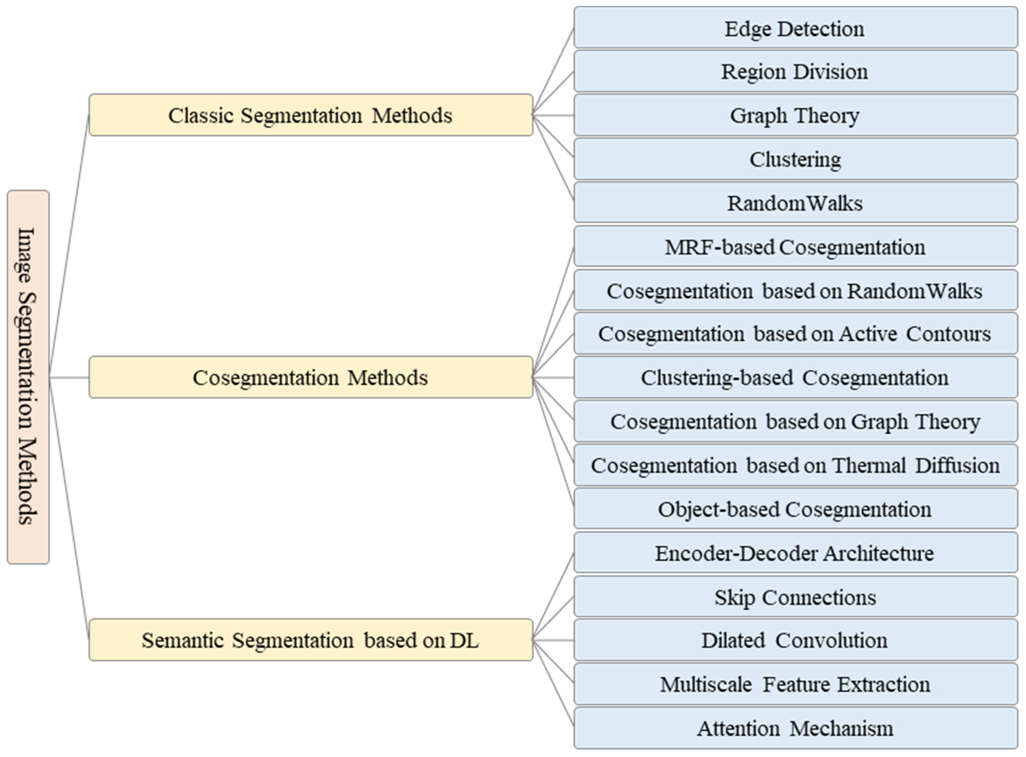
2. Classic Segmentation Methods
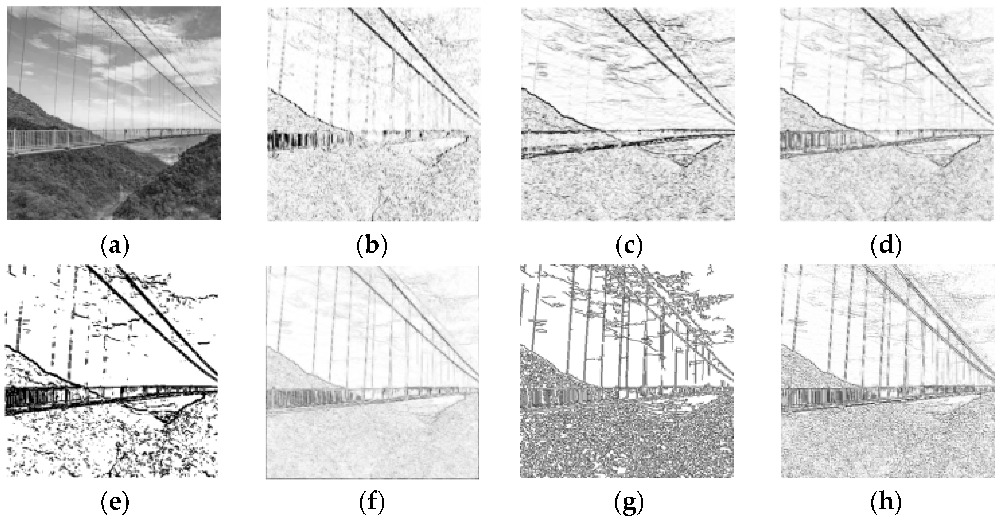
The classic segmentation algorithms were proposed for grayscale images, which mainly consider gray-level similarity in the same region and gray-level discontinuity in different regions. In general, region division is based on gray-level similarity, and edge detection is based on gray-level discontinuity. Color image segmentation involves using the similarity between pixels to segment the image into different regions or superpixels, and then merging these superpixels.

2.1. Edge Detection

The positions where the gray level changes sharply in an image are generally the boundaries of different regions. The task of edge detection is to identify the points on these boundaries. Edge detection is one of the earliest segmentation methods and is also called the parallel boundary technique. The derivative or differential of the gray level is used to identify the obvious changes at the boundary. In practice, the derivative of the digital image is obtained by using the difference approximation for the differential. Examples of edge detection results are represented in Figure 2.
These operators are sensitive to noise and are only suitable for images with low noise and complexity. The Canny operator performs best among the operators shown in Figure 2. It has strong denoising ability, and also processes the segmentation of lines well with continuity, fineness, and straightness. However, the Canny operator is more complex and takes longer to execute. In the actual industrial production, a thresholding gradient is usually used in the case of high real-time requirement. On the contrary, the more advanced Canny operator is selected in the case of high quality requirement.
Although differential operators can locate the boundaries of different regions efficiently, the closure and continuity of the boundaries cannot be guaranteed due to numerous discontinuous points and lines in the high-detail regions. Therefore, it is necessary to smooth the image before using a differential operator to detect edges.
Another edge detection method is the serial boundary technique, that concatenates points of edges to form a closed boundary. Serial boundary techniques mainly include graph-searching algorithms and dynamic programming algorithms. In graph-searching algorithms, the points on the edges are represented by a graph structure, and the path with the minimum cost is searched in the graph to determine the closed boundaries, which is always computationally intensive. The dynamic programming algorithm utilizes heuristic rules to reduce the search computation.
The active contours method approximates the actual contours of the objects by matching the closed curve (i.e., the initial contours based on gradient) with the local features of the image, and finds the closed curve with the minimum energy by minimizing the energy function to achieve image segmentation. The method is sensitive to the location of the initial contour, so the initialization must be close to the target contour. Moreover, its non-convexity easily leads to the local minimum, so it is difficult to converge to the concave boundary. Lankton and Tannenbaum [9] proposed a framework that considers the local segmentation energy to evolve contours, that could produce the initial localization according to the locally based global active contour energy and effectively segment objects with heterogeneous feature profiles.
Graph cuts marks the target nodes (i.e., source nodes) and background nodes (i.e., sink nodes), and uses the vector connection between different nodes to represent the fit degree of the nodes and the corresponding pixels (i.e., the penalty function). Graph cuts is an NP-hard problem, so efficient approximation algorithms must be sought to minimize the energy function, that can be adopted by using a swap algorithm based on the semi-metric properties of connections and an expansion algorithm based on the metric properties of nodes. Freedman [10] proposed an interactive segmentation graph cuts algorithm combined with the prior knowledge of shapes, that solved the problems to a certain extent of inaccurate segmentation in the case of diffuse edges or multiple close similar objects. Graph cuts algorithms are widely used in the field of medical image analysis.

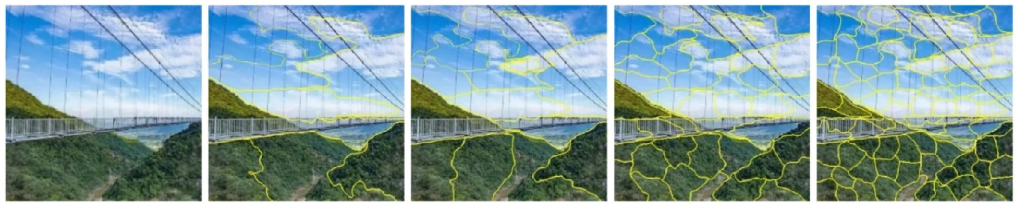
2.2. Region Division

The region division strategy includes serial region division and parallel region division. Thresholding is a typical parallel region division algorithm. The threshold is generally defined by the trough value in a gray histogram with some processing to make the troughs in the histogram deeper or to convert the troughs into peaks. The optimal grayscale threshold can be determined by the zeroth-order or first-order cumulant moment of the gray histogram to maximize the discriminability of the different categories.
The serial region technique involves dividing the region segmentation task into multiple steps to be performed sequentially, and the representative steps are region growing and region merging.
Region growing involves taking multiple seeds (single pixels or regions) as initiation points and combining the pixels with the same or similar features in the seed neighborhoods in the regions where the seed is located, according to a predefined growth rule until no more pixels can be merged. The principle of region merging is similar to the region growing, except that region merging measures the similarity by judging whether the difference between the average gray value of the pixels in the region obtained in the previous step and the gray value of its adjacent pixels is less than the given threshold K . Region merging can be used to solve the problem of hard noise loss and object occlusion, and has a good effect on controlling the segmentation scale and processing unconventional data; however, its computational cost is high, and the stopping rule is difficult to affirm.
Watershed is based on the concept of topography. When water rises from a low place, dams need to be built to prevent the water from reaching the mountain peaks. The dams built on the mountain peaks divide the entire image into several regions. The watershed algorithm can obtain the closed contour and has high processing efficiency. However, when the image is more complex, it is prone to false segmentation, that can be solved by establishing a Gaussian mixture model (GMM). The improved watershed has high generalization performance, is often used in the segmentation of MRI images and digital elevation maps, and is especially effective for segmenting medical images containing overlapping cells (e.g., blood cell segmentation).
The superpixel is a series of small irregular areas composed of pixels with similar positions and features (e.g., brightness, color, and texture). Using superpixels instead of pixels to represent features can reduce the complexity of image processing, so it is often used in the preprocessing of image segmentation. Image segmentation methods based on superpixel generation mainly include clustering and graph theory.

2.3. Graph Theory

The image segmentation method based on graph theory maps an image to a graph, that represents pixels or regions as vertices of the graph, and represents the similarity between vertices as weights of edges. Image segmentation, based on graph theory, is regarded as the division of vertices in the graph, analyzing the weighted graph with the principle and method based on graph theory, and obtaining optimal segmentation with the global optimization of the graph (e.g., the min-cut).
Graph-based region merging uses different metrics to obtain optimal global grouping instead of using fixed merging rules in clustering. Felzenszwalb et al. [11] used the minimum spanning tree (MST) to merge pixels after the image was represented as a graph.
Image segmentation based on MRF (Markov random field) introduces probabilistic graphical models (PGMs) into the region division to represent the randomness of the lower-level features in the images. It maps the image to an undigraph, where each vertex in the graph represents the feature at the corresponding location in the image, and each edge represents the relationship between two vertices. According to the Markov property of the graph, the feature of each point is only related to its adjacent features.
Leordeanu et al. [12] proposed a method based on spectral graph partitioning to find the correspondence between two sets of features. Adjacency matrix M is built for the weighted graph corresponding to the image, and the mapping constraints required for the overall mapping are imposed on the principal eigenvectors of M , so that the correct assignments are recovered according to the strong degree of the main cluster of M .

2.4. Clustering Method

K-means clustering is a special thresholding segmentation algorithm that is proposed based on the Lloyd algorithm. The algorithm operates as follows: (i) initialize K points as clustering centers; (ii) calculate the distance between each point i in the image and K cluster centers, and select the minimum distance as the classification k i ; (iii) average the points of each category (the centroid) and move the cluster center to the centroid; and (iv) repeat steps (ii) and (iii) until algorithm convergence. Simply put, K-means is an iteration process for computing the cluster centers. The K-means has noise robustness and quick convergence, but it is not conducive to processing nonadjacent regions, and it can only converge to the local optimum solution instead of the global optimum solution.
Mean-shift [13] is a clustering algorithm based on density estimation, that models the image feature space to the probability density function. Chuang [14] proposed a fuzzy C-means algorithm that integrated spatial information into the membership function for clustering to generate more uniform region segmentation.
Spectral clustering is a common clustering method based on graph theory, that divides the weighted graph and creates subgraphs with low coupling and high cohesion. Achanta et al. [15] proposed a simple linear iterative clustering (SLIC) algorithm that used K-means to generate superpixels; its segmentation results are shown in Figure 3. SLIC can be applied to 3D supervoxel generation. Li et al. [16] proposed a superpixel segmentation algorithm named linear spectral clustering (LSC), that used a kernel function to map the coordinates of the pixel values into a high-dimensional space, and weighted each point in the feature space appropriately to obtain the same optimal solution for both the objective function of K-means and the normalized cut.

2.5. Random Walks

Random walks is a segmentation algorithm based on graph theory, that is commonly used in image segmentation, image denoising [17,18], and image matching [19]. By assigning labels to adjacent pixels in accordance with predefined rules, pixels with the same label can be represented together to distinguish different objects.
Grady et al. [20] transformed the segmentation problem into a discrete Dirichlet problem. They converted the image into a connected undigraph with weight, and marked the foreground and background of the image with one or a group of points, respectively, as initial conditions. For the unmarked points, they calculated the probability of reaching the foreground and background for the first time in random walks, and then took the highest probability as its category. Yang et al. [21] proposed a constrained random walks algorithm, that took user input as subsidiary conditions, e.g., users could assign the foreground and background in the image, or draw the regions where the boundaries must pass (hard constraint) or the regions where the boundaries can pass or not (soft constraint). The framework contained a constrained random walks algorithm and a local edit algorithm, that resulted in more accurate region contours and interoperability.
Lai et al. [22] extended the random walks image segmentation idea to 3D mesh images. They represented each side of the mesh as a vertex in the graph, defined the weight of edges by using the dihedral angle between adjacent faces, and sought a harmonic function adapted to boundary conditions. On this basis, Zhang et al. [23] proposed a fast geodesic curvature flow (FGCF) algorithm, that considered mesh vertices as the graph vertices to reduce the number of vertices in the graph, and changed the cutting contour to the local minimum of the weighted curve to smooth the zigzag contour. Therefore, the FGCF with less user input permitted had increased efficiency and higher robustness in the segmentation of the mesh benchmark dataset.

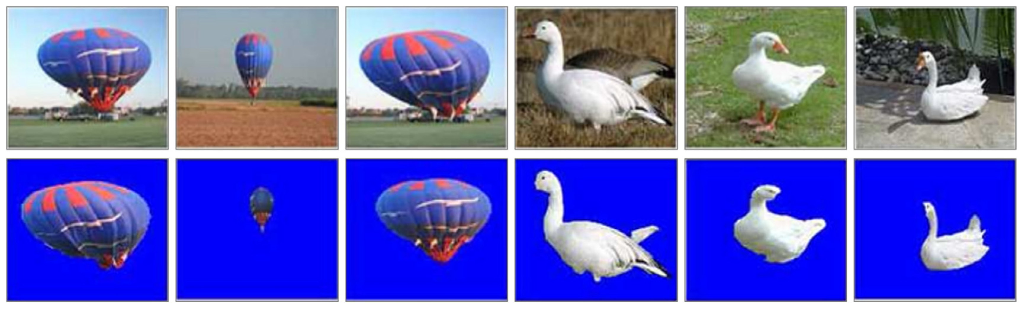
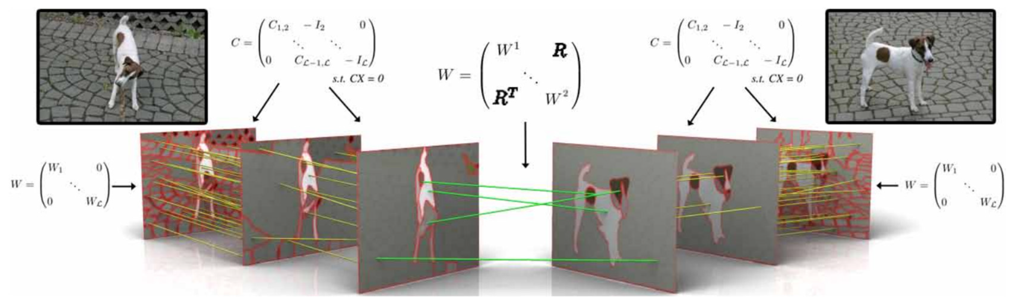
3. Co-Segmentation Methods

The classic segmentation methods usually focus on the feature extraction of a single image, which makes it difficult to obtain the high-level semantic information of the image. In 2006, Rother et al. [24] proposed the concept of collaborative segmentation for the first time. Collaborative segmentation, or co-segmentation for short, involves extracting the common foreground regions from multiple images with no human intervention, to obtain prior knowledge. Figure 4 shows a set of examples of co-segmentation results.
To achieve co-segmentation, it is necessary to extract the features of the foreground of single or multiple images (the seed image(s)) as prior knowledge using a classic segmentation method, and then utilize the prior knowledge to process a set of images containing the same or similar objects. The extended model can be expressed as follows:
E = E s + E g
where E s represents the energy function of seed image segmentation, that describes the difference between the foreground and background of the image and the smoothness of the image, and E g represents the energy function of co-segmentation, that describes the similarity between foregrounds in a set of images. To achieve a good co-segmentation effect, segmentation energy E should be minimized. This can be achieved using two methods: improving the classic segmentation method to minimize E s , or optimizing the unsupervised learning method to learn good representations in image sets to minimize E g .
The energy function in the classic segmentation model is E s . e.g., when using MRF segmentation method as E s , then
E s M R F = E u M R F + E p M R F
where E u M R F and E p M R F are the unary potential and the pairwise potential, respectively. The former measures the properties of the pixel itself, and the latter measures itself in relation to other pixels. In MRF, the unary potential represents the probability of a pixel belonging to class x i when a feature of the pixel is y i , which is x i E u ( x i ) ; the pairwise potential represents the probability that two adjacent pixels belong to the same category, which is x i , x j Ψ E p ( x i , x j ) . The co-segmentation term E g is used to penalize the inconsistency of multiple foreground color histograms. In the MRF-based co-segmentation models, multifarious co-segmentation terms and their minimization methods were proposed.

3.1. MRF-Based Co-Segmentation

Rother et al. [24] extended the MRF segmentation and utilized prior knowledge to solve the ill-posed problems in multiple image segmentation. First, they segmented the foreground of the seed image, and assumed that the foreground objects of a set of images are similar; then, they built the energy function according to the consistency of the MRF probability distribution and the global constraint of the foreground feature similarity; finally, they estimated whether each pixel belongs to the foreground or background by minimizing the energy function to achieve the segmentation of the foreground and background.
The subsequent research on MRF co-segmentation focused on the optimization of global constraints. Vicente et al. [25] proposed an extended Boykov–Jolly model using multiscale decomposition, based on the L1 norm model [24], the L2 norm model [26], and the reward model [27]. Compared with the above three models, the extended Boykov–Jolly model made great strides in reducing the number of parameters and improving robustness. Rubio et al. [28] evaluated the foreground similarity through high-order graph matching and introduced high-order graph matching into the MRF model to form global terms. Chang et al. [29] proposed a universal significance measure for images as prior knowledge, that could add foreground positional information in the MRF model and solve the problem of significant differences in the appearance, shape, and scale of multiple images. Yu et al. [30] adopted a method combined with a co-saliency model to achieve co-segmentation, and they represented the dissimilarity between foreground objects in each image and common objects in the dataset with a Gaussian mixture model as a new global constraint, then added the global constraint to co-segmentation energy E, and used graph cuts to minimize the energy function iteratively.
The co-segmentation based on MRF has good universality, and it is commonly used in video object detection and segmentation [30,31] and interactive image editing [32].

3.2. Co-Segmentation Based on Random Walks

Collins et al. [33] extended the random walks model to solve the co-segmentation problem, further utilized the quasiconvexity to optimize the segmentation algorithm, and provided a professional CUDA library to calculate the linear operation of the image sparse features. Fabijanska et al. [34] proposed an optimized random walks algorithm for 3D voxel image segmentation, using a supervoxel instead of a single voxel, which greatly saved computing time and memory resources. Dong et al. [35] proposed a subMarkov random walks (subRW) algorithm with prior label knowledge, which combined subRW with other random walks algorithms for seed image segmentation, and it achieved a good segmentation effect on images containing slender objects.
The co-segmentation methods based on random walks have good flexibility and robustness. They have achieved good results in some areas of medical image segmentation, especially in 3D medical image segmentation [36,37].

3.3. Co-Segmentation Based on Active Contours

Meng et al. [38] extended the active contour method to co-segmentation, constructed an energy function based on foreground consistency between images and background inconsistency within each image, and solved the energy function minimization by level set. Zhang et al. [39] proposed a deformable co-segmentation algorithm which transformed the prior heuristic information of brain anatomy contained in multiple images into the constraints controlling the brain MRI segmentation, and acquired the minimum energy function by level set, solving the problem of brain MRI image segmentation. Zhang et al. [40] introduced the saliency of the region of interest in the image into the active contour algorithm to improve the effect of the co-segmentation of multiple images, and proposed a level set optimization method based on superpixels, hierarchical computing, and convergence judgment to solve the minimized energy function.
The co-segmentation methods based on active contours have a good effect on the boundary extraction of complex shapes, but their unidirectional movement characteristic severely limits their flexibility, which is not conducive to the recognition and processing of objects with weak edges.

3.4. Clustering-Based Co-Segmentation

Clustering-based co-segmentation is an extension of the clustering segmentation of a single image. Joulin et al. [41] proposed a co-segmentation method based on spectral clustering and discriminative clustering. They used spectral clustering to segment a single image based on local spatial information, and then used discriminative clustering to propagate the segmentation results in a set of images to achieve co-segmentation. Kim et al. [42] divided the image into superpixels, used a weighted graph to describe the relevance of superpixels, converted the weighted graph into an affinity matrix to describe the relation of the intra-image, and then adopted spectral clustering to achieve co-segmentation. This final representation can be seen in Figure 5.
If the number of initial cluster centers is not limited, the clustering method can be applied to the multi-objective co-segmentation problem. The algorithm follows the processes below. Firstly, the image is segmented into local regions of multiple superpixel blocks through image preprocessing. Then, these local regions are clustered by a clustering algorithm to form the corresponding prior information. Finally, the prior information is propagated in a set of images to achieve multi-object co-segmentation. Joulin et al. [43] used a similarity matrix based on feature positions and color vectors to represent the local information in a single image; that is, spectral clustering. According to the local information and feature mapping relation, the expectation maximization (EM) was used to minimize the classification discriminant function to obtain a set of parameters. The algorithm could realize multiple classes and a significantly larger number of image co-segmentations effectively.

3.5. Co-Segmentation Based on Graph Theory

Co-segmentation based on graph theory partitions an image into a digraph.
In contrast to the digraph mentioned earlier, Meng et al. [44] divided each image into several local regions based on the object detection, and then used these local regions as nodes to construct a digraph instead of using superpixels or pixels as nodes. Nodes are connected by directed edges, and the weight of the edges represents the local region similarity and saliency map between the two objects. Thereupon, the image co-segmentation problem was converted into the problem of finding the shortest path on the digraph. Finally, they obtained the shortest path through the dynamic programming (DP) algorithm. The flowchart is shown in Figure 6.
In the same year, Meng et al. [45] proposed a new co-saliency model to extract co-saliency maps from pairwise-constrained images. The co-saliency map consists of two terms; that is, the saliency map based on a single image and the saliency map based on multiple images, so it can also be called a dual-constrained saliency map. Compared to [44], the co-saliency map obtained by pairwise-constrained graph matching is more accurate. They extracted multiple saliency maps by matching similar regions between images, transformed it into a pairwise-constrained graph matching problem, and solved the pairwise-constrained graph matching problem using the DP algorithm.

3.6. Co-Segmentation Based on Thermal Diffusion

Thermal diffusion image segmentation maximizes the temperature of the system by changing the location of the heat source, and its goal is to find the optimal location of the heat source to achieve the best segmentation effect. Anisotropic diffusion is a nonlinear filter that can not only reduce the Gaussian noise but also preserve image edges. It is often used in image processing to reduce noise while enhancing image details. Kim et al. [46] proposed a method called CoSand, that adopted temperature maximization modeling on anisotropic diffusion, where k heat sources maximize the temperature corresponding to the segmentation of k-categories; they achieved large-scale multicategory co-segmentation by maximizing the segmentation confidence of each pixel in the image. Kim et al. [47] realized multi-foreground co-segmentation by iteratively implementing the two tasks of scene modeling and region labeling according to the similarity of the foreground objects in multiple images. In the process of foreground modeling, a spatial pyramid matching algorithm was used to extract local features, the linear support vector machine (SVM) was used for feature matching, and the Gaussian mixture model was used for object classification and detection. This method achieved good evaluation results on the Flickr MFC and ImageNet, and was still accurately segmented when foreground objects did not appear in every image.

3.7. Object-Based Co-Segmentation

Alexe et al. [48] proposed an object-based measurement method to quantify the possibility that an image window contains objects of any category. The probability of whether it is an object in each sampling window was calculated in advance, and the highest scoring window was used as the feature calibration for each category of objects according to the Bayesian theory. The method could distinguish between objects with clear spatial boundaries, e.g., telephones, as well as amorphous background elements, e.g., grass, that greatly reduced the number of specified category object detection windows. Vicente et al. [49] used foreground objects, measured the similarity between objects, extracted the features with the highest score from multiple candidate object classes, and achieved good experimental results on the iCoseg dataset.
To solve the problem of multi-object segmentation, binary segmentation methods based on target similarity ranking were proposed, that built a model using the maximum flow of parameters and trained a scoring function to obtain the optimal prediction result. The scoring function is determined by the properties, e.g., the convexity of all objects in the foreground, the continuity of the curve, the contrast between the foreground and the background, and the positions of the objects in the image. Meng et al. [50] proposed a multi-group image co-segmentation framework, that could obtain inter-image information in each set of images, generating more accurate prior knowledge; they used MRF and the dense mapping model, used EM to solve the energy E minimization problem of co-segmentation, and achieved the co-segmentation of multiple foreground recognition. The main methods in co-segmentation are shown in Table 1.

4. Semantic Segmentation Based on Deep Learning

With the continuous development of image acquisition equipment, there has been a great increase in the complexity of image details and the difference in objects (e.g., scale, posture). Low-level features (e.g., color, brightness, and texture) are difficult to obtain good segmentation results from, and feature extraction methods based on manual or heuristic rules cannot meet the complex needs of current image segmentation, that puts forward the higher generalization ability of image segmentation models.
Semantic texton forests [51] and random forest [52] methods were generally used to construct semantic segmentation classifiers before deep learning was applied to the field of image segmentation. For the past few years, deep learning algorithms have been increasingly applied to segmentation tasks, and the segmentation effect and performance have been significantly improved. The original approach divides the image into small patches to train a neural network and then classifies the pixels. This patch classification algorithm [53] has been adopted because the fully connected layers of the neural network require fixed-size images.
In 2015, Long et al. [54] proposed fully convolutional networks (FCNs) with convolution instead of full connection, that made it possible to input any image size, and the FCN architecture is shown in Figure 7. FCNs prove that neural networks can perform end-to-end semantic segmentation training, laying a foundation for deep neural networks in semantic segmentation.
Subsequent networks were advanced based on the FCN model. The following section introduces the main technologies and representative models from the perspective of how semantic segmentation networks work. The main semantic segmentation algorithms based on deep learning are shown in Table 2.

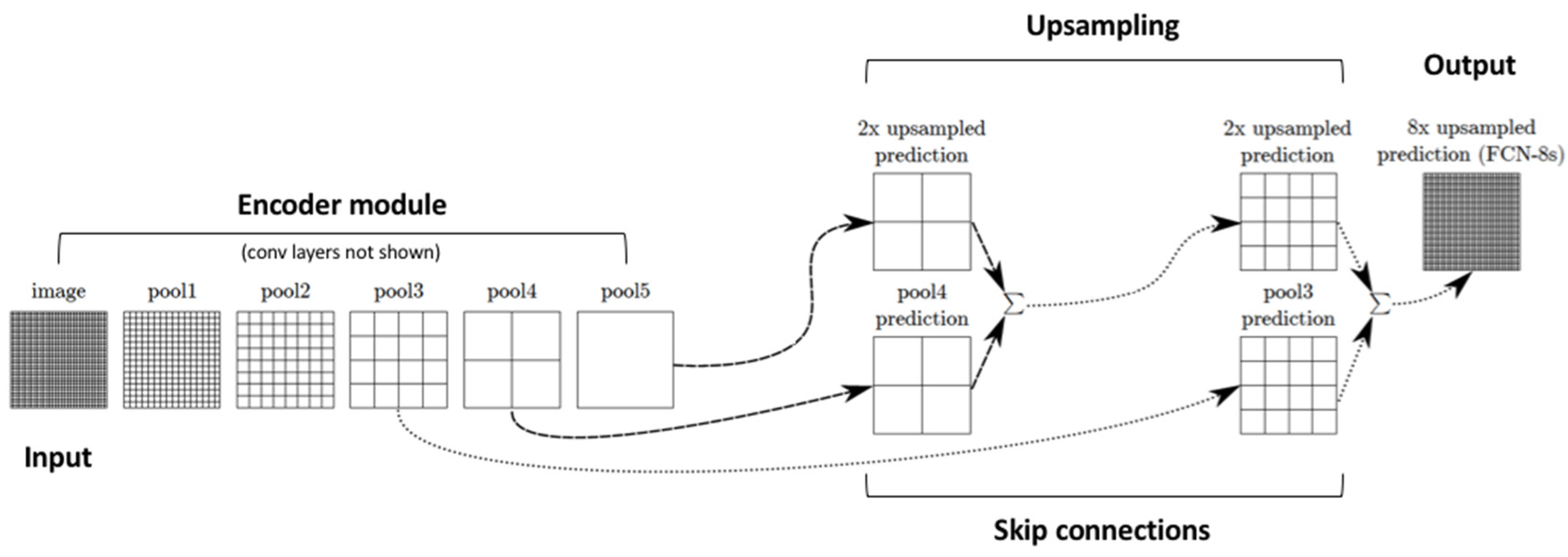
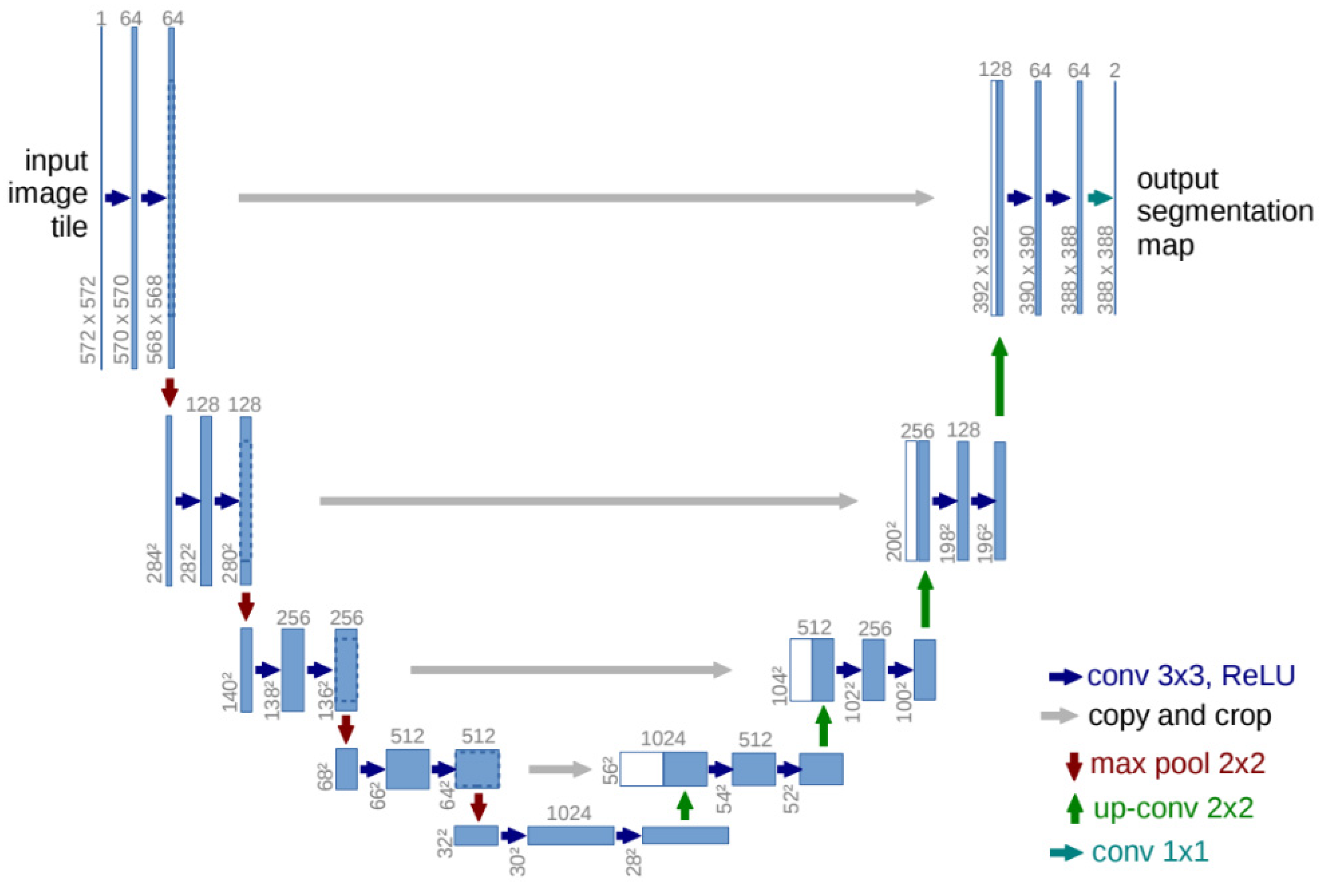
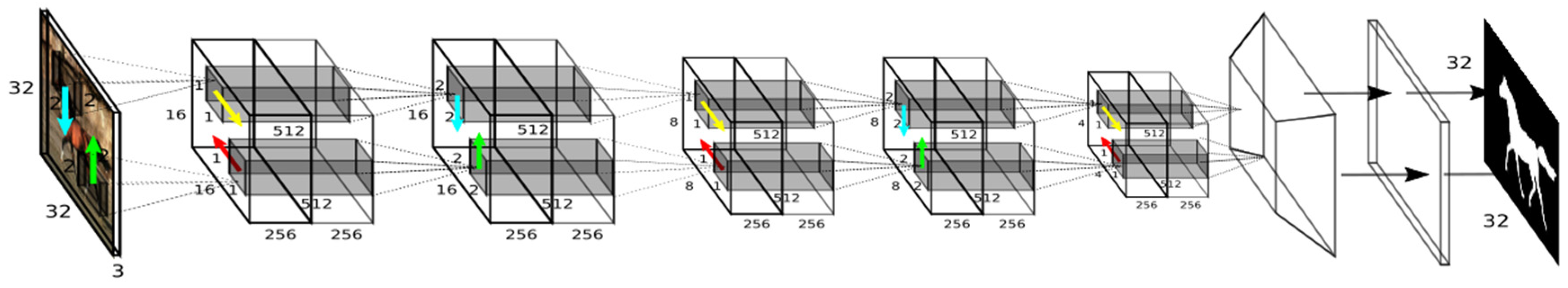
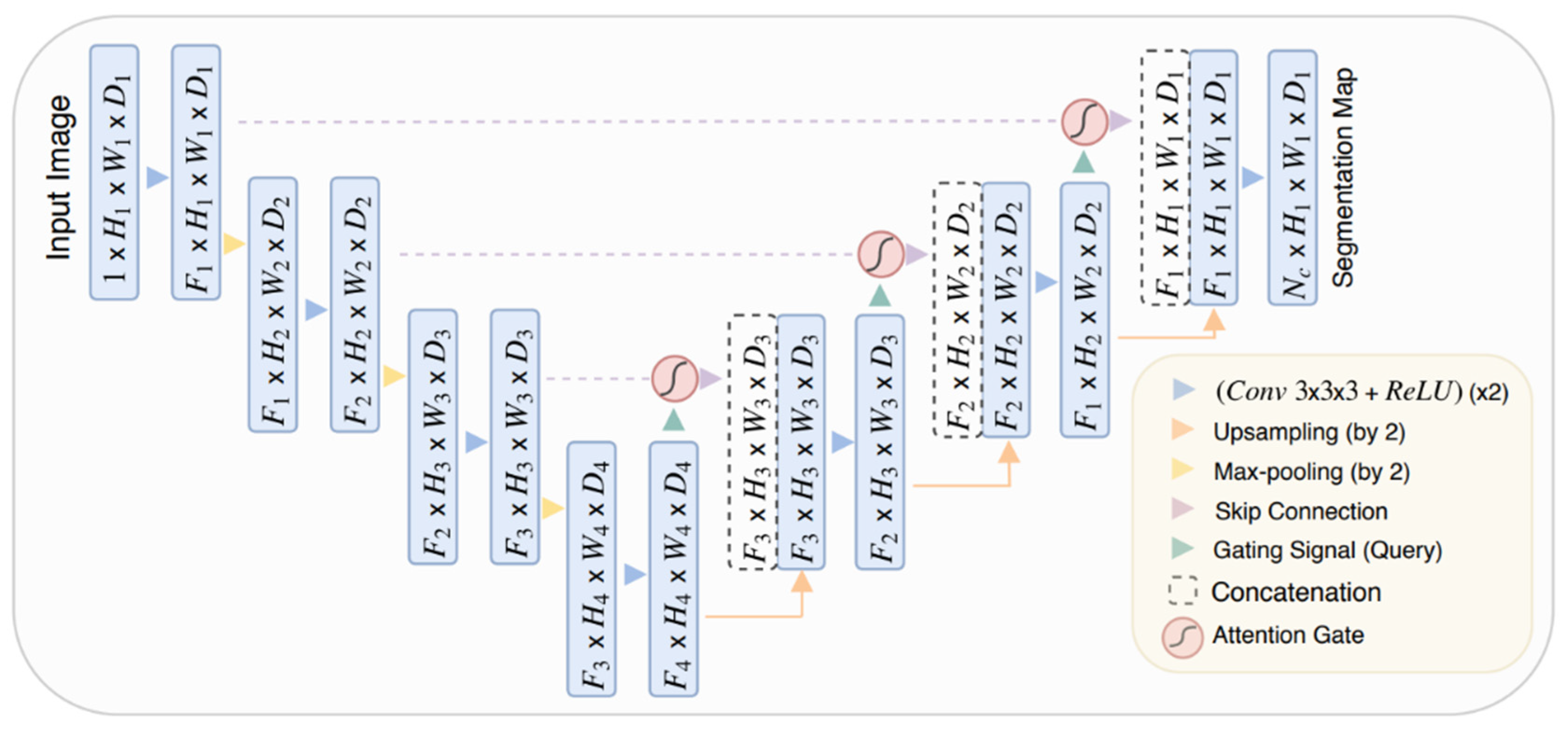
4.1. Encoder–Decoder Architecture

Encoder–decoder architecture is based on FCNs. Prior to FCNs, convolutional neural networks (CNNs) achieved good effects in image classification, e.g., LeNet-5 [55], AlexNet [56], and VGG [57], whose output layers are the categories of images. However, semantic segmentation needs to map the high-level features back to the original image size after obtaining high-level semantic information. This requires an encoder–decoder architecture.
In the encoder stage, convolution and pooling operations are mainly performed to extract high-dimensional features containing semantic information. The convolution operation involves performing the multiplication and summing of the image-specific region with different convolution kernels pixel-for-pixel, and then transforming the activation function to obtain a feature map. The pooling operation involves sampling within a certain region (the pooling window), and then using a certain sampling statistic as the representative feature of the region. The backbone blocks commonly used in segmentation network encoders are VGG, Inception [58,59], and ResNet [60].
In the decoder stage, an operation is performed to generate a semantic segmentation mask by the high-dimensional feature vector. The process to map back the multi-level features extracted by the encoder to the original image is called up-sampling.
  • The interpolation method uses a specified interpolation strategy to insert new elements between the pixels of the original image, thereby expanding the size of the image and achieving the effect of up-sampling. Interpolation does not require training parameters and is often used in early up-sampling tasks;
  • The FCN adopts deconvolution for up-sampling. Deconvolution, also known as transposed convolution, reverses the parameters of the original convolution kernel upside down and flipped horizontally, and fills the spaces between and around the elements of the original image;
  • SegNet [61] adopts the up-sampling method of unpooling. Unpooling represents the inverse operation of max-pooling in the CNN. During maximum pooling, not only the maximum value of the pooling window, but also the coordinate position of the maximum values should be recorded; in the case of unpooling, the maximum value of this position is activated, and the values in other positions are all set to 0;
  • Wang et al. [62] proposed a dense up-sampling convolution (DUC), the core idea of which is to convert the label mapping in the feature map into smaller label mapping with multiple channels. This transformation can be achieved by directly using convolutions between the input feature map and the output label map, without the need to interpolate extra values during the up-sampling process.

4.2. Skip Connections

Skip connections or shortcut connections were developed to improve rough pixel positioning. With deep neural network training, the performance decreases as the depth increases, which is a degradation problem. To ameliorate this problem, different skip connection structures have been proposed in ResNet and DenseNet [63]. In contrast, U-Net [64] proposed a new long skip connection, as shown in Figure 8. U-Net makes jump connections and cascades of features from layers in the encoder to the corresponding layers in the decoder to obtain the fine-grained details of images. It was proposed to solve the problem of annotations in image segmentation based on biological microscopes, and it has since been widely used in research on medical image segmentation.

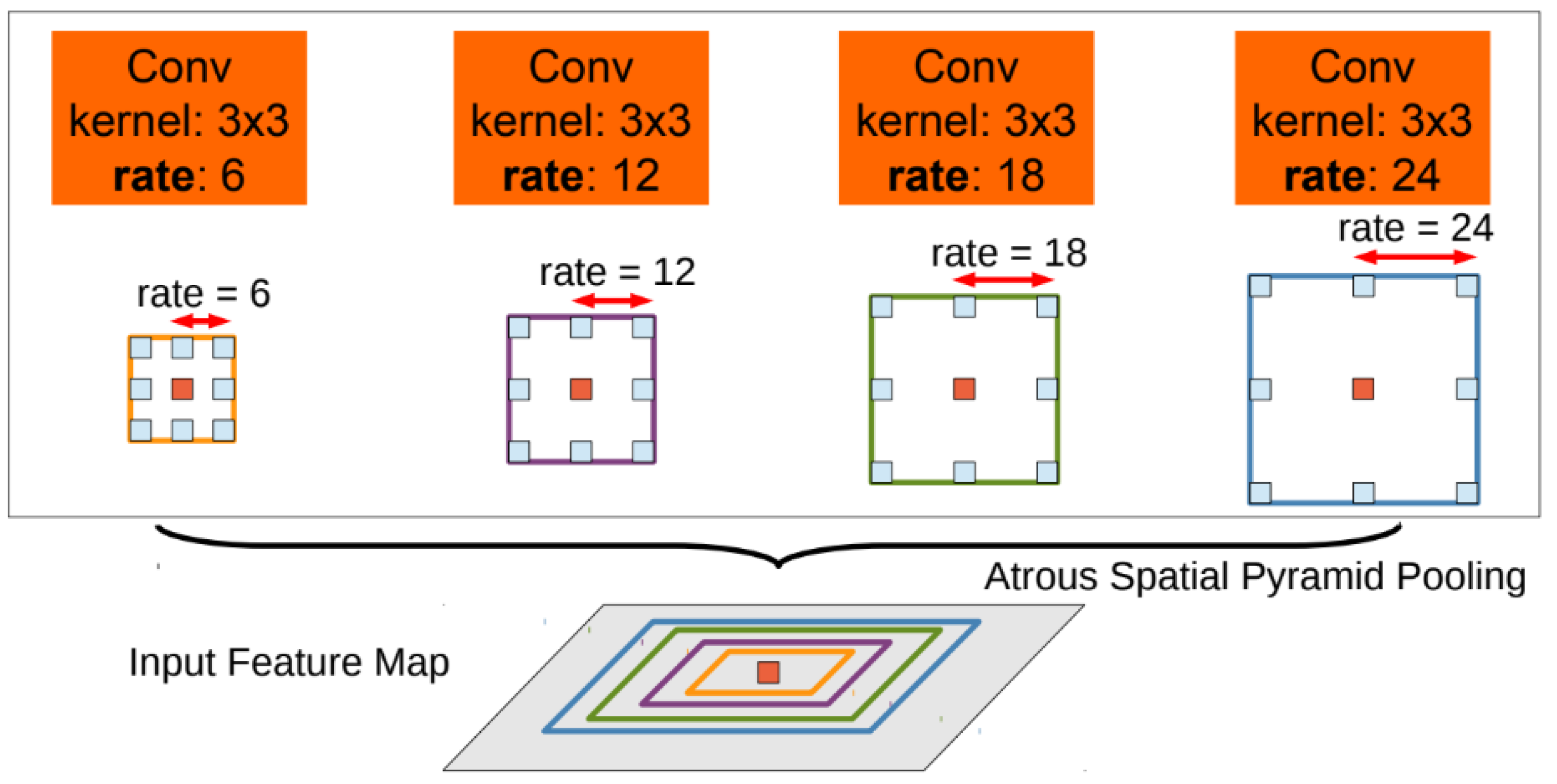
4.3. Dilated Convolution

Dilated convolution, also known as atrous convolution, is constructed by inserting holes into the convolution kernel to expand the receptive field and reduce the computation during down-sampling. In FCN, the max-pooling layers are replaced by dilated convolution to maintain the receiving field of the corresponding layer and the high resolution of the feature map.
The DeepLab series [65,66,67,68] are classic models in the field of semantic segmentation. Prior to putting forward DeepLab V1, the semantic segmentation results were usually rough due to the transfer invariance lost in the pooling process, and the probabilistic relationship between labels not used for prediction. To ameliorate these problems, DeepLab V1 [65] uses dilated convolution to solve the problem of resolution reduction during up-sampling, and uses fully connected conditional random fields (fully connected CRFs) to optimize the post-processing of segmented images to obtain objects at multi-scales and context information.
Yu et al. [69] used dilated convolution to aggregate multiscale context information. They adopted a context module with eight convolutional layers, among which seven layers applied different 3 × 3 convolution kernels with different dilation factors (i.e., [1, 1, 2, 4, 8, 16, 1]), that proved that the simplified adaptive network could further improve the accuracy and precision of image segmentation without any resolution being lost. In [70], they proposed a dilated residual network (DRN) based on ResNet, that included five groups of convolutional layers. The down-sampling of the latter two groups (i.e., G4 and G5) was removed to maintain the spatial resolution of the feature map. Instead of this, the subsequent convolutions of G4 and G5 used dilated convolutions with dilatation rates r = 2 and r = 4 , respectively.
Wang et al. [62] proposed a hybrid dilated convolution (HDC) to effectively deal with the “gridding” problem caused by dilated convolution. The HDC makes the final size of the receptive field of a series of convolution operations completely cover a square region without any holes or missing edges. To enable this, they used a different dilation rate for each layer, instead of using the same dilation rate for all layers after previous down-sampling.

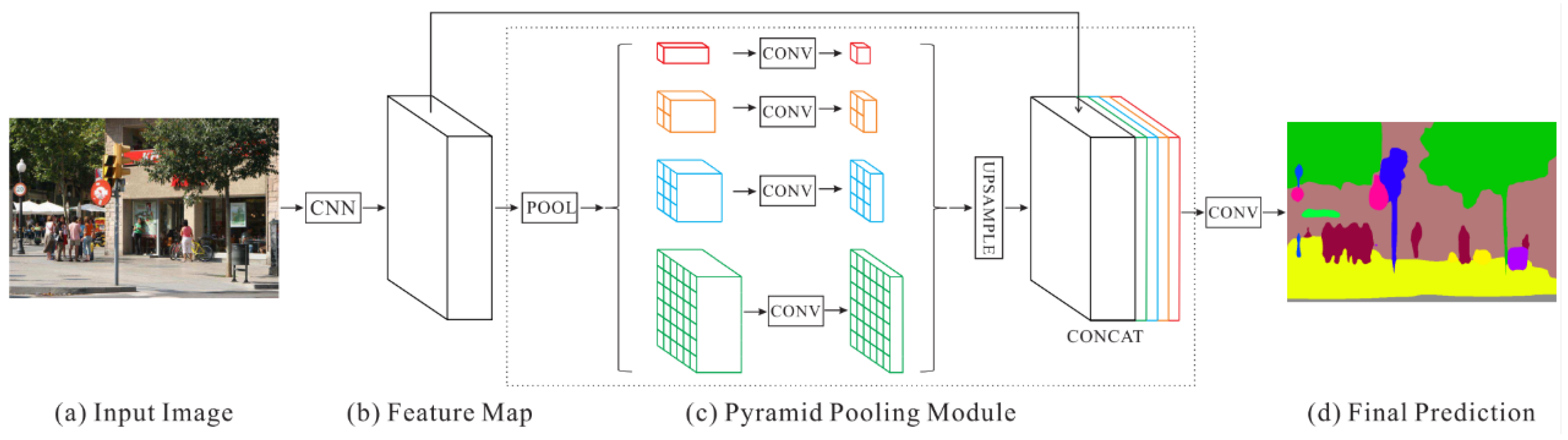
4.4. Multiscale Feature Extraction

Spatial pyramid pooling (SPP) was proposed to solve the problem of the CNNs requiring fixed-size input images. He et al. [71] developed the SPP-net and verified its effectiveness in semantic segmentation and object detection. To make the most of image context information, Zhao et al. [72] developed PSPNet with a pyramid pooling module (PPM), as shown in Figure 9. Using ResNet as the backbone network, the PSPNet utilized PPM to extract and aggregate different subregion features at different scales, that were then up-sampled and concatenated to form the feature map, that carried both local and global context information. It is particularly worth noting that the number of pyramid layers and the size of each layer are variable, that depend on the size of the feature map input to the PPM.
Ghiasi and Fowlkes [73] described a multi-resolution reconstruction architecture based on a Laplacian pyramid, that used skip connections from higher-resolution feature maps and multiplicative gating to refine segmentation boundaries reconstructed from lower-resolution maps successively.
DeepLab V2 [66] introduced atrous spatial pyramid pooling (ASPP) to expand the receptive field and capture multiscale features. The ASPP module contained four parallel dilated convolutions with different dilation rates, as shown in Figure 10. Referring to the HDC method, DeepLab V3 [67] applied both cascade modules and parallel modules of dilated convolution, grouped the parallel convolution in the ASPP module, and added the 1 × 1 convolution layer and batch normalization in the ASPP module. The DeepLab V3 significantly improved on the previous DeepLab versions without DenseCRF post-processing. Moreover, using Xception as the backbone network and DeepLab V3 as the decoder, DeepLab V3+ [68] adopted dilated depth wise separable convolutions instead of max-pooling and batch normalization to refine the segmentation boundaries.
The scheme of FPN (feature pyramid network) [74] is similar to the skip connections of the U-Net model, that is beneficial for obtaining high resolution and strong semantic features for object detection with significant size differences in the images. He et al. [75] proposed an adaptive pyramid context network (APCNet) to solve the optimal solution of semantic segmentation. They utilized multiple adaptive context modules (ACMs) to build multiscale contextual feature representations; each ACM used the global image representation to estimate the local affinity weights of each subregion and calculated the optimal context vector according to these local affinity weights.
Ye et al. [76] developed an enhanced feature pyramid network (EFPN), that combined a semantic enhancement module (SEM), edge extraction module (EEM), and context aggregation model (CAM) into a decoder network to improve the robustness of multi-level feature fusion, and added a global fusion model (GFM) into the encoder network to capture more deep semantic information and transmit it to each layer efficiently. Among them, the SEM upgraded the ASPP module by modifying smaller dilation rates to enhance and obtain low-level features and replacing the pooling layer with a short residual connection in post-processing to avoid the loss of shallow semantic information, that simplified the network with a denser connection.
Wu et al. [77] proposed FPANet, a feature pyramid aggregation network for real-time semantic segmentation. FPANet is also an encoder–decoder model, using ResNet and ASPP in the encoder stage and a semantic bidirectional feature pyramid network (SeBiFPN) in the decoder stage. Reducing the number of feature channels with a lightweight feature pyramid fusion module (FPFM), the SeBiFPN was utilized to obtain both the semantic and spatial information of images and fuse features of different levels.

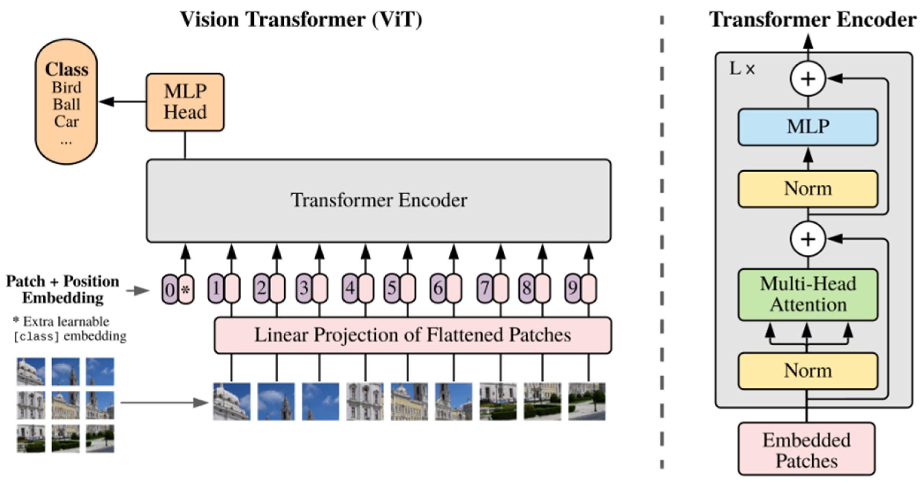
4.5. Attention Mechanisms

To represent the dependency between different regions in an image, especially the long-distance regions, and obtain their semantic relevance, some methods commonly used in the field of natural language processing (NLP) have been applied to computer vision, that have made good achievements in semantic segmentation. The attention mechanism was first put forward in the computer vision field in 2014. The Google Mind team [78] adopted the recurrent neural network (RNN) model to apply attention mechanisms to image classification, making attention mechanisms gradually popular in image processing tasks.
RNN can model the short-term dependence between pixels, connect pixels, and process them sequentially, which establishes a global context relationship. Visin et al. [79] proposed a ReSeg network based on ReNet [80], and each ReNet layer consisted of four RNNs that swept in both horizontal and vertical directions across the image to obtain global information. The ReSeg architecture is shown in Figure 11.
LSTM (long short-term memory) adds a new function to record long-term memory, that can represent long-distance dependence. Byeon et al. [81] used LSTM to achieve pixel-for-pixel segmentation of scene images, which proved that image texture information and spatial model parameters could be learned in a 2D LSTM model. Liang et al. [82] proposed a semantic segmentation model based on the graph LSTM model, that extended LSTM from sequential data or multidimensional data to a general graph structure, further enhancing the global context visual features.
Both RNN and LSTM have their limitations, e.g., weakened long-distance dependence, requiring too many parameters, and not allowing parallel operations. Oktay et al. [83] proposed attention U-Net, as shown in Figure 12, that introduced an attention mechanism in U-Net. Prior to splicing the features at each resolution of the encoder with the corresponding features in the decoder, they used attention gate (AG) modules to supervise the features of the previous layer through the features of the next layer, thus readjusting the output features of the encoder. The AG modules adjusted the activation value adaptively by generating a gated signal and suppressed the feature responses of the unrelated background regions progressively to control the importance of different spatial features. Pal et al. [84] proposed an attention UW-Net, that achieved a good performance on medical chest X-ray images. The attention UW-Net improves a skip connection based on the U-Net segmentation network, i.e., a dense connection is added between the B-5 and B-6 blocks of the original U-Net architecture, that allows the network to learn the details lost in the previous max-pooling and effectively reduces the information loss. In addition, an improved attention gate is designed, that modifies the resampling of the attention vectors by copying the vector space in the channel attention, which could better realize the attention to the salient region and the suppression of the irrelevant background region.
Self-attention mechanisms are mostly used in the encoder network to represent the correlation between different regions (pixels) or different channels of the feature maps. It computes a weighted sum of pairwise affinities across all positions of a single sample to update the feature at each position. Self-attention mechanisms have produced many influential achievements in image segmentation, e.g., PSANet [85], DANet [86], APCNet [75], CARAFE [87], and CARAFE++ [88].
In 2017, Vaswani et al. [89] proposed the transformer, a deep neural network solely based on a self-attention mechanism, dispensing with convolutions and recurrence entirely. Thereafter, transformer and its variants (i.e., X-transformer) were used in the field of computer vision. With the self-attention mechanism of the transformer and CNN pre-training model, the improved network [90,91] achieved some breakthroughs. Dosovitskiy et al. [92] proposed a vision transformer (ViT), that proved that transformer could substitute for CNN in classification and prediction of image patch sequences. As shown in Figure 13, they divided the image into patches of fixed sizes, lined up the image patches, and input the patches sequence vector into a transformer encoder (the right-hand diagram), that consisted of alternating multi-head attention layers and multi-layer perceptron (MLP).
Liu et al. [93] developed the swin transformer, that has achieved impressive performance in image semantic segmentation and instance segmentation. The swin transformer advanced the sliding window approach, that built hierarchical feature maps by merging image patches in deeper layers, calculated self-attention in each local window, and utilized cyclic-shifting window partition approaches alternatively in the consecutive swin transformer blocks to introduce cross-window connections between neighboring non-overlapping windows. The swin transformer network replaced the standard multi-head self-attention (MSA) module in a transformer block with shifted window approach, with the other layers remaining the same, as shown in Figure 14.
Figure 14. The architecture of a swin transformer. Figure from [93].
Electronics 12 01199 g014
Table 2. Comparison and analysis of semantic segmentation methods based on deep learning.
AlgorithmsPub. YearBackboneExperimentsMajor Contributions
DatasetsmIoU (%)
FCN [54]2015VGG-16PASCAL VOC 201162.7The forerunner for end-to-end semantic segmentation
NYUDv234.0
U-Net [64]2015VGG-16PhC-U37392.03Encoder–decoder structure,
skip connections
DIC-HeLa77.56
SegNet [61]2016VGG-16CamVid60.4Transferred the max-pooling indices to the decoder
SUN RGBD28.27
DeepLabv1 [65]2016VGG-16PASCAL VOC 201271.6Atrous convolution, fully connected CRFs
MSCA [88]2016VGG-16PASCAL VOC 201275.3Dilated convolutions, multi-scale context aggregation, front-end context module
LRR [73]2016ResNet/VGG-16PASCAL VOC 201177.5Reconstruction up-sampling module, Laplacian pyramid refinement
Cityscapes69.7
ReSeg [79]2016VGG-16 & ReNetCamVid91.6Extension of ReNet to semantic segmentation
Oxford Flowers93.7
CamVid58.8
DRN [70]2017ResNet-101Cityscapes70.9Modified Conv4/5 of ResNet,
dilated convolution
PSPNet [72]2017ResNet50PASCAL VOC 201285.4Spatial pyramid pooling (SPP)
Cityscapes80.2
DeepLab V2 [66]2017VGG-16/ResNet-101PASCAL VOC 201279.7Atrous spatial pyramid pooling (ASPP), fully connected CRFs
Cityscapes70.4
DeepLab V3 [67]2017ResNet-101PASCAL VOC 201286.9Cascaded or parallel ASPP modules
Cityscapes81.3
DeepLab V3+ [68]2018XceptionPASCAL VOC 201289.0A new encoder–decoder structure with DeepLab V3 as an encoder
Cityscapes82.1
DUC-HDC [62]2018ResNet-101/ResNet-152PASCAL VOC 201283.1HDC (hybrid dilation convolution) was proposed to solve the gridding caused by dilated convolutions
Cityscapes80.1
Attention U-Net [83]2018VGG-16 with AGsmulti-class abdominal CT-150--A novel self-attention gating (AGs) filter, skip connections
TCIA Pancreas CT-82--
PSANet [85]2018ResNet-101ADE20K81.51Point-wise spatial attention maps from two parallel branches, bi-direction information propagation model
PASCAL VOC 201285.7
Cityscapes81.4
APCNet [75]2019ResNet-101PASCAL VOC 201284.2Multi-scale, global-guided local affinity (GLA), adaptive context modules (ACMs)
PASCAL Context54.7
ADE20K45.38
DANet [86]2019ResNet-101Cityscapes81.5Dual attention: position attention module and channel attention module
PASCAL VOC 201282.6
PASCAL Context52.6
COCO Stuff39.7
CARAFE [87]2019ResNet-50ADE20k42.23Pyramid pooling module (PPM), feature pyramid network (FPN), multi-level feature fusion (FUSE)
EFPN [76]2021VGG-16PASCAL VOC 201286.4PPM, multi-scale feature fusion module with a parallel branch
Cityscapes82.3
PASCAL Context53.9
CARAFE++ [88]2021ResNet-101ADE20k43.94PPM, FPN, FUSE, adaptive kernels on-the-fly
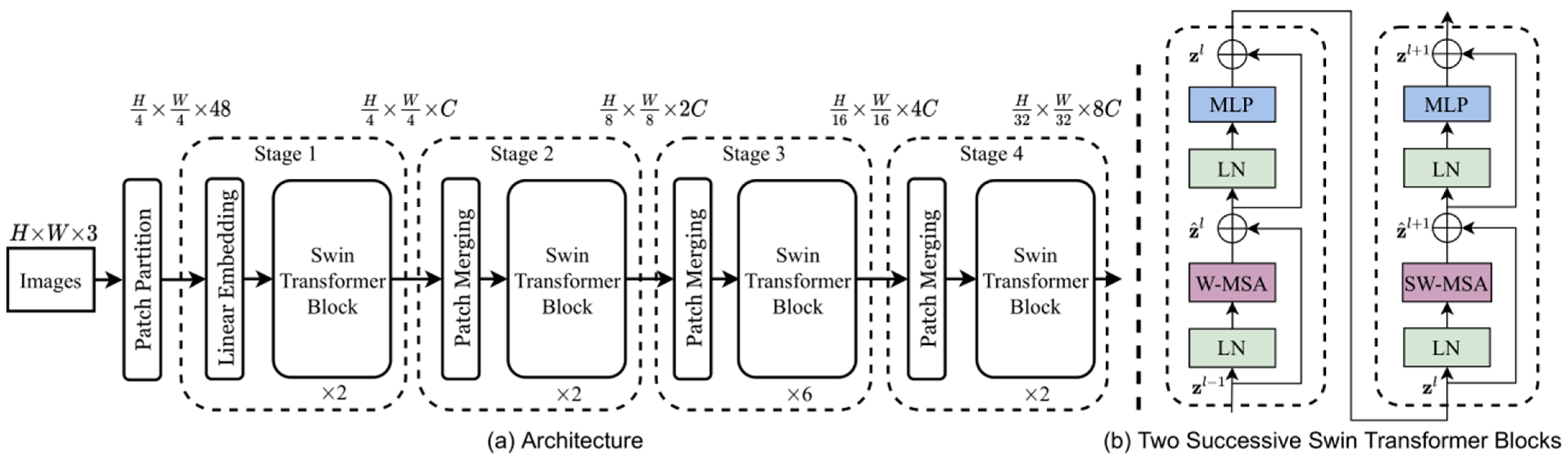
Swin Transformer [93]2021Swin-LSwin-L53.5A novel shifted windowing scheme, a general backbone network for computer vision
Attention UW-Net [84]2022ResNet50NIH Chest X-ray--Skip connections,
an intermediate layer that combines the feature maps of the fourth-layer encoder with the feature maps of the last-layer encoder layer,
attention mechanism
FPANet [77]2022ResNet18Cityscapes75.9Bilateral directional FPN, lightweight ASPP, feature pyramid fusion module (FPFM), border refinement module (BRM)
CamVid74.7

5. Conclusions

According to the chronological evolution of image segmentation technology, we have comprehensively sorted the classic segmentation algorithms and the current popular deep learning algorithms, elaborated on the representative solutions of each stage, and enumerated the classic algorithms with certain influences. In general, the development of image segmentation shows a trend from coarse-grained to fine-grained, from manual feature extraction to adaptive learning, and from single-image-oriented to segmentation based on common features of big data.
With the development of image acquisition technology, the types of images are becoming more varied, that brings more challenges in image segmentation with different dimensions, scales, resolutions, and imaging modes. Researchers expect the use of a general network with improved adaptability and generalization ability [94]. Since the FCN was proposed, deep neural network research has shown obvious advantages in scene understanding and object recognition. Future research directions still focus on deep neural networks, aiming to further improve the accuracy, real-time ability, and robustness of the network. With the great breakthrough made by the swin transformer in the field of computer vision in 2021, image segmentation has entered the transformer stage from the CNN stage, and the transformer may bring new advances to computer vision research. Nevertheless, deep learning also has its shortcomings, e.g., deep learning is inexplicable, which limits the robustness, reliability, and performance optimization of its downstream tasks. The current research directions and challenges of image segmentation are as follows:
  • Semantic segmentation, instance segmentation, and panoramic segmentation are still the research hotspots of image segmentation. Instance segmentation predicts the pixel regions contained in each instance; panoramic segmentation integrates both semantic segmentation and instance segmentation, and assigns a category label and an instance ID to each pixel of the image. Especially in panoramic segmentation, countable, or uncountable instances are difficult to recognize in a single workflow, so it is a challenging task to build an effective network to simultaneously identify both large inter-category differences and small intra-category differences;
  • With the popularization of image acquisition equipment (e.g., LiDAR cameras), RGB-depth, 3D-point clouds, voxels, and mesh segmentation have gradually become research hotspots, which have a wide requirement in face recognition [95], autonomous vehicles, VR, AR, architectural modeling, etc. Although there has been some progress in the research of 3D image segmentation, e.g., region growth, random walks, and clustering in classic algorithms, and SVM, random forest, and AdaBoost in machine learning algorithms, the representation and processing of 3D data, which are unstructured, redundant, disordered, and unevenly distributed, remain a major challenge;
  • In some fields, it is difficult to use supervised learning algorithms to train the network due to a lack of datasets or fine-grained annotations. Semi-supervised and unsupervised semantic segmentation can be selected in these cases, where the network can be trained on the benchmark dataset first, and the lower-level parameters of the network can then be fixed, and the fully connected layer or some high-level parameters can be trained on the small-sample dataset. This is transfer learning, that does not require abundant labeled samples. Reinforcement learning is also a possible solution, but it is rarely studied in the field of image segmentation. In addition, few-shot image semantic segmentation is also a hot research direction;
  • Deep learning networks require a significant amount of computing resources in the training process, that also illustrates the computational complexity of the deep neural network. Real-time (or near real-time) segmentation is required in many fields, e.g., video processing to meet the human vision mechanism of at least 25 fps, and most current networks are far below this frame rate. Some lightweight networks have improved the speed of the segmentation to a certain extent, but there is still a large amount of room for improvement in the balance of model accuracy and real-time performance.

Author Contributions

Conceptualization, C.W. and Q.F.; methodology, C.W. and Q.F.; investigation, R.K. and F.H.; resources, Q.F.; data curation, B.Y., T.Y. and M.G.; writing—original draft preparation, Y.Y.; writing—review and editing, Y.Y. and C.W.; supervision, Q.F. and M.G.; project administration, C.W. and Q.F.; funding acquisition, Q.F. and F.H. All authors have read and agreed to the published version of the manuscript.

Funding

This research was supported by the National Natural Science Foundation of China (No. 62171467), the Hainan Provincial Natural Science Foundation of China (No. 621QN270), and the Specific Research Fund of The Innovation Platform for Academicians of Hainan Province (No. YSPTZX202144).

Data Availability Statement

Not applicable.

Acknowledgments

The authors gratefully acknowledge Dongdong Zhang, Changfeng Feng, and Huiying Wang for their fruitful discussions.

Conflicts of Interest

The authors declare no conflict of interest.

References

  1. Anwesh, K.; Pal, D.; Ganguly, D.; Chatterjee, K.; Roy, S. Number plate recognition from enhanced super-resolution using generative adversarial network. Multimed. Tools Appl. 2022, 1–17. [Google Scholar] [CrossRef]
  2. Jin, B.; Cruz, L.; Gonçalves, N. Deep Facial Diagnosis: Deep Transfer Learning from Face Recognition to Facial Diagnosis. IEEE Access 2020, 8, 123649–123661. [Google Scholar] [CrossRef]
  3. Zhao, M.; Liu, Q.; Jha, R.; Deng, R.; Yao, T.; Mahadevan-Jansen, A.; Tyska, M.J.; Millis, B.A.; Huo, Y. VoxelEmbed: 3D Instance Segmentation and Tracking with Voxel Embedding based Deep Learning. In Proceedings of the International Workshop on Machine Learning in Medical Imaging, Strasbourg, France, 27 September 2021; Volume 12966, pp. 437–446. [Google Scholar] [CrossRef]
  4. Yao, T.; Qu, C.; Liu, Q.; Deng, R.; Tian, Y.; Xu, J.; Jha, A.; Bao, S.; Zhao, M.; Fogo, A.B.; et al. Compound Figure Separation of Biomedical Images with Side Loss. In Proceedings of the Deep Generative Models, and Data Augmentation, Labelling, and Imperfections, Strasbourg, France, 1 October 2021; Volume 13003, pp. 173–183. [Google Scholar] [CrossRef]
  5. Minaee, S.; Boykov, Y.; Porikli, F.; Plaza, A.; Kehtarnavaz, N.; Terzopoulos, D. Image Segmentation Using Deep Learning: A Survey. IEEE Trans. Pattern Anal. Mach. Intell. 2022, 44, 3523–3542. [Google Scholar] [CrossRef] [PubMed]
  6. Zhang, X.; Yao, Q.A.; Zhao, J.; Jin, Z.J.; Feng, Y.C. Image Semantic Segmentation Based on Fully Convolutional Neural Network. Comput. Eng. Appl. 2022, 44, 45–57. [Google Scholar]
  7. Garcia-Garcia, A.; Orts-Escolano, S.; Oprea, S.; Villena-Martinez, V.; Martinez-Gonzalez, P.; Garcia-Rodriguez, J. A survey on deep learning techniques for image and video semantic segmentation. Appl. Soft Comput. 2018, 70, 41–65. [Google Scholar] [CrossRef]
  8. Yu, Y.; Wang, C.; Fu, Q.; Kou, R.; Wu, W.; Liu, T. A Survey of Evaluation Metrics and Methods for Semantic Segmentation. Comput. Eng. Appl. 2023; online preprint. [Google Scholar]
  9. Lankton, S.; Tannenbaum, A. Localizing Region-Based Active Contours. IEEE Trans. Image Process. 2008, 17, 2029–2039. [Google Scholar] [CrossRef] [Green Version]
  10. Freedman, D.; Tao, Z. Interactive Graph Cut based Segmentation with Shape Priors. In Proceedings of the IEEE Computer Society Conference on Computer Vision and Pattern Recognition (CVPR), San Diego, CA, USA, 20–25 June 2005; Volume 1, pp. 755–762. [Google Scholar] [CrossRef] [Green Version]
  11. Felzenszwalb, P.F.; Huttenlocher, D.P. Efficient Graph-Based Image Segmentation. Int. J. Comput. Vis. 2004, 59, 167–181. [Google Scholar] [CrossRef]
  12. Leordeanu, M.; Hebert, M. A Spectral Technique for Correspondence Problems using Pairwise Constraints. In Proceedings of the 10th IEEE International Conference on Computer Vision (ICCV’05), Beijing, China, 17–21 October 2005; Volume 2, pp. 1482–1489. [Google Scholar] [CrossRef] [Green Version]
  13. Comaniciu, D.; Meer, P. Mean Shift: A Robust Approach Toward Feature Space Analysis. IEEE Trans. Pattern Anal. Mach. Intell. 2002, 24, 603–619. [Google Scholar] [CrossRef] [Green Version]
  14. Chuang, K.S.; Tzeng, H.L.; Chen, S.; Wu, J.; Chen, T.J. Fuzzy C-means Clustering with Spatial Information for Image Segmentation. Comput. Med. Imaging Graph. Off. J. Comput. Med. Imaging Soc. 2006, 30, 9–15. [Google Scholar] [CrossRef] [Green Version]
  15. Achanta, R.; Shaji, A.; Smith, K.; Lucchi, A.; Fua, P.; Süsstrunk, S. SLIC Superpixels Compared to State-of-the-Art Su-perpixel Method. IEEE Trans. Pattern Anal. Mach. Intell. 2012, 34, 2274–2282. [Google Scholar] [CrossRef] [Green Version]
  16. Li, Z.; Chen, J. Superpixel Segmentation using Linear Spectral Clustering. In Proceedings of the 2015 IEEE Conference on Computer Vision and Pattern Recognition (CVPR), Boston, MA, USA, 7–12 June 2015; pp. 1356–1363. [Google Scholar] [CrossRef]
  17. Pan, W.; Lu, X.Q.; Gong, Y.H.; Tang, W.M.; Liu, J.; He, Y.; Qiu, G.P. HLO: Half-kernel Laplacian Operator for Sur-face Smoothing. Comput. Aided Des. 2020, 121, 102807. [Google Scholar] [CrossRef] [Green Version]
  18. Chen, H.B.; Zhen, X.; Gu, X.J.; Yan, H.; Cervino, L.; Xiao, Y.; Zhou, L.H. SPARSE: Seed Point Auto-Generation for Random Walks Segmentation Enhancement in medical inhomogeneous targets delineation of morphological MR and CT images. J. Appl. Clin. Med. Phys. 2015, 16, 387–402. [Google Scholar] [CrossRef] [PubMed]
  19. Drouyer, S.; Beucher, S.; Bilodeau, M.; Moreaud, M.; Sorbier, L. Sparse Stereo Disparity Map Densification using Hierarchical Image Segmentation. In Mathematical Morphology and Its Applications to Signal and Image Processing; Lecture Notes in Computer Science; Springer: Berlin/Heidelberg, Germany, 2017; Volume 1022. [Google Scholar] [CrossRef]
  20. Grady, L. Random Walks for Image Segmentation. IEEE Trans. Pattern Anal. Mach. Intell. 2006, 28, 1768–1783. [Google Scholar] [CrossRef] [PubMed] [Green Version]
  21. Yang, W.; Cai, J.; Zheng, J.; Luo, J. User-Friendly Interactive Image Segmentation Through Unified Combinatorial User Inputs. IEEE Trans. Image Process. 2010, 19, 2470–2479. [Google Scholar] [CrossRef] [PubMed]
  22. Lai, Y.K.; Hu, S.M.; Martin, R.R.; Rosin, P.L. Fast Mesh Segmentation using Random Walks. In Proceedings of the 2008 ACM Symposium on Solid and Physical Modeling, New York, NY, USA, 2 June 2008; pp. 183–191. [Google Scholar] [CrossRef] [Green Version]
  23. Zhang, J.; Wu, C.; Cai, J.; Zheng, J.; Tai, X. Mesh Snapping: Robust Interactive Mesh Cutting using Fast Geodesic Curvature Flow. Comput. Graph. Forum 2010, 29, 517–526. [Google Scholar] [CrossRef]
  24. Rother, C.; Minka, T.P.; Blake, A.; Kolmogorov, V. Cosegmentation of Image Pairs by Histogram Matching—Incorporating a Global Constraint into MRFs. In Proceedings of the IEEE Computer Society Conference on Computer Vision and Pattern Recognition (CVPR), New York, NY, USA, 17–22 June 2006; pp. 993–1000. [Google Scholar] [CrossRef]
  25. Vicente, S.; Kolmogorov, V.; Rother, C. Cosegmentation Revisited: Models and Optimization. Lecture Notes in Computer Science. In Proceedings of the Computer Vision (ECCV), Crete, Greece, 5–11 September 2010; pp. 465–479. [Google Scholar] [CrossRef] [Green Version]
  26. Mukherjee, L.; Singh, V.; Dyer, C.R. Half-integrality-based Algorithms for Cosegmentation of Images. In Proceedings of the IEEE Conference on Computer Vision and Pattern Recognition (CVPR), Miami, FL, USA, 20–25 June 2009; pp. 2028–2035. [Google Scholar] [CrossRef]
  27. Hochbaum, D.S.; Singh, V. An Efficient Algorithm for Co-segmentation. In Proceedings of the 12th IEEE International Con-ference on Computer Vision (ICCV), Kyoto, Japan, 29 September–2 October 2009; pp. 269–276. [Google Scholar] [CrossRef] [Green Version]
  28. Rubio, J.C.; Serrat, J.; López, A.; Paragios, N. Unsupervised Co-segmentation through Region Matching. In Proceedings of the 2012 IEEE Conference on Computer Vision and Pattern Recognition (CVPR), Providence, RI, USA, 16–21 June 2012; pp. 749–756. [Google Scholar] [CrossRef]
  29. Chang, K.; Liu, T.; Lai, S. From Co-saliency to Co-segmentation: An Efficient and Fully Unsupervised Energy Minimization Model. In Proceedings of the 24th IEEE Conference on Computer Vision and Pattern Recognition (CVPR), Colorado Springs, CO, USA, 20–25 June 2011; pp. 2129–2136. [Google Scholar] [CrossRef] [Green Version]
  30. Yu, H.; Xian, M.; Qi, X. Unsupervised Co-segmentation based on a New Global GMM Constraint in MRF. In Proceedings of the IEEE International Conference on Image Processing (ICIP), Paris, France, 27–30 October 2014; pp. 4412–4416. [Google Scholar] [CrossRef]
  31. Wang, C.; Guo, Y.; Zhu, J.; Wang, L.; Wang, L. Video Object Co-Segmentation via Subspace Clustering and Quadratic Pseudo-Boolean Optimization in an MRF Framework. IEEE Trans. Multimed. 2014, 16, 903–916. [Google Scholar] [CrossRef]
  32. Zhu, J.; Wang, L.; Gao, J.; Yang, R. Spatial-Temporal Fusion for High Accuracy Depth Maps using Dynamic MRFs. IEEE Trans. Pattern Anal. Mach. Intell. 2010, 32, 899–909. [Google Scholar] [CrossRef]
  33. Collins, M.D.; Xu, J.; Grady, L.; Singh, V. Random Walks based Multi-image Segmentation: Quasiconvexity Results and GPU-based Solutions. In Proceedings of the 2012 IEEE Conference on Computer Vision and Pattern Recognition, Providence, RI, USA, 16–21 June 2012; pp. 1656–1663. [Google Scholar] [CrossRef] [Green Version]
  34. Fabijanska, A.; Goclawski, J. The Segmentation of 3D Images using the Random Walking Technique on a Randomly Created Image Adjacency Graph. IEEE Trans. Image Process. 2015, 24, 524–537. [Google Scholar] [CrossRef]
  35. Dong, X.P.; Shen, J.B.; Shao, L.; Gool, L.V. Sub-Markov Random Walk for Image Segmentation. IEEE Trans. Image Process. 2016, 25, 516–527. [Google Scholar] [CrossRef] [Green Version]
  36. Zhou, J.; Wang, W.M.; Zhang, J.; Yin, B.C.; Liu, X.P. 3D shape segmentation using multiple random walkers. J. Comput. Appl. Math. 2018, 329, 353–363. [Google Scholar] [CrossRef]
  37. Dong, C.; Zeng, X.; Lin, L.; Hu, H.; Han, X.; Naghedolfeizi, M.; Aberra, D.; Chen, Y.W. An Improved Random Walker with Bayes Model for Volumetric Medical Image Segmentation. J. Healthc. Eng. 2017, 2017, 6506049. [Google Scholar] [CrossRef] [PubMed] [Green Version]
  38. Meng, F.; Li, H.; Liu, G. Image Co-segmentation via Active Contours. In Proceedings of the 2012 IEEE International Symposium on Circuits and Systems (ISCAS), Seoul, Republic of Korea, 20–23 May 2012; pp. 2773–2776. [Google Scholar] [CrossRef]
  39. Zhang, T.; Xia, Y.; Feng, D.D. A Deformable Cosegmentation Algorithm for Brain MR Images. In Proceedings of the Annual International Conference of the IEEE Engineering in Medicine and Biology Society, San Diego, CA, USA, 28 August–1 September 2012; pp. 3215–3218. [Google Scholar] [CrossRef]
  40. Zhang, Z.; Liu, X.; Soomro, N.Q.; Abou-El-Hossein, K. An Efficient Image Co-segmentation Algorithm based on Active Contour and Image Saliency. In Proceedings of the 2016 7th International Conference on Mechanical, Industrial, and Manufacturing Technologies (MIMT 2016), Cape Town, South Africa, 1–3 February 2016; Volume 54, p. 08004. [Google Scholar] [CrossRef] [Green Version]
  41. Joulin, A.; Bach, F.; Ponce, J. Discriminative Clustering for Image Co-segmentation. In Proceedings of the 2010 IEEE Computer Society Conference on Computer Vision and Pattern Recognition (CVPR), San Francisco, CA, USA, 13–18 June 2010; pp. 1943–1950. [Google Scholar] [CrossRef] [Green Version]
  42. Kim, E.; Li, H.; Huang, X. A Hierarchical Image Clustering Cosegmentation Framework. In Proceedings of the IEEE Computer Society Conference on Computer Vision and Pattern Recognition (CVPR), Providence, RI, USA, 16–21 June 2012; pp. 686–693. [Google Scholar] [CrossRef]
  43. Joulin, A.; Bach, F.; Ponce, J. Multi-class Cosegmentation. In Proceedings of the 2012 IEEE Conference on Computer Vision and Pattern Recognition (CVPR), Providence, RI, USA, 16–21 June 2012; pp. 542–549. [Google Scholar] [CrossRef]
  44. Meng, F.; Li, H.; Liu, G.; Ngan, K.N. Object Co-Segmentation Based on Shortest Path Algorithm and Saliency Model. IEEE Trans. Multimed. 2012, 14, 1429–1441. [Google Scholar] [CrossRef]
  45. Meng, F.M.; Li, H.; Liu, G.H. A New Co-saliency Model via Pairwise Constraint Graph Matching. In Proceedings of the International Symposium on Intelligent Signal Processing and Communications Systems, Tamsui, Taiwan, 4–7 November 2012; IEEE Computer Society Press: Los Alamitos, CA, USA, 2012; pp. 781–786. [Google Scholar] [CrossRef]
  46. Kim, G.; Xing, E.P.; Li, F.F.; Kanade, T. Distributed Cosegmentation via Submodular Optimization on Anisotropic Diffusion. In Proceedings of the 2011 International Conference on Computer Vision, Barcelona, Spain, 6–13 November 2011; pp. 169–176. [Google Scholar] [CrossRef]
  47. Kim, G.; Xing, E.P. On Multiple Foreground Cosegmentation. In Proceedings of the 2012 IEEE Conference on Computer Vision and Pattern Recognition, Providence, RI, USA, 16–21 June 2012; pp. 837–844. [Google Scholar] [CrossRef]
  48. Alexe, B.; Deselaers, T.; Ferrari, V. What Is an Object? In Proceedings of the 2010 IEEE Computer Society Conference on Computer Vision and Pattern Recognition, San Francisco, CA, USA, 13–18 June 2010; pp. 73–80. [Google Scholar] [CrossRef]
  49. Vicente, S.; Rother, C.; Kolmogorov, V. Object cosegmentation. In Proceedings of the IEEE Computer Society Conference on Computer Vision and Pattern Recognition (CVPR), Colorado Springs, CO, USA, 20–25 June 2011. [Google Scholar] [CrossRef]
  50. Meng, F.; Cai, J.; Li, H. Cosegmentation of Multiple Image Groups. Comput. Vis. Image Underst. 2016, 146, 67–76. [Google Scholar] [CrossRef]
  51. Johnson, M.; Shotton, J.; Cipolla, R. Semantic Texton Forests for Image Categorization and Segmentation. In Decision Forests for Computer Vision and Medical Image Analysis, Advances in Computer Vision and Pattern Recognition; Criminisi, A., Shotton, J., Eds.; Springer: London, UK, 2013. [Google Scholar] [CrossRef] [Green Version]
  52. Lindner, C.; Thiagarajah, S.; Wilkinson, J.M.; The arcOGEN Consortium; Wallis, G.A.; Cootes, T.F. Fully Automatic Segmentation of the Proximal Femur using Random Forest Regression Voting. IEEE Trans. Med. Imaging 2013, 32, 1462–1472. [Google Scholar] [CrossRef]
  53. Li, H.S.; Zhao, R.; Wang, X.G. Highly Efficient Forward and Backward Propagation of Convolutional Neural Networks for Pixelwise Classification. arXiv 2014, arXiv:1412.4526. [Google Scholar]
  54. Long, J.; Shelhamer, E.; Darrell, T. Fully Convolutional Networks for Semantic Segmentation. IEEE Trans. Pattern Anal. Mach. Intell 2017, 39, 640–651. [Google Scholar] [CrossRef]
  55. Lecun, Y.; Bottou, L.; Bengio, Y.; Haffner, P. Gradient-based Learning Applied to Document Recognition. Proc. IEEE 1998, 86, 2278–2324. [Google Scholar] [CrossRef] [Green Version]
  56. Krizhevsky, A.; Sutskever, I.; Hinton, G.E. ImageNet Classification with Deep Convolutional Neural Networks. Commun. ACM 2017, 60, 84–90. [Google Scholar] [CrossRef] [Green Version]
  57. Karen, S.; Andrew, Z. Very Deep Convolutional Networks for Large-Scale Image Recognition. arXiv 2014, arXiv:1409.1556. [Google Scholar]
  58. Szegedy, C.; Liu, W.; Jia, Y.Q.; Sermanet, P.; Reed, S.; Anguelov, D.; Erhan, D.; Vanhoucke, V.; Rabinovich, A. Going Deeper with Convolutions. In Proceedings of the 2015 IEEE Conference on Computer Vision and Pattern Recognition (CVPR), Boston, MA, USA, 7–12 June 2015; pp. 1–9. [Google Scholar] [CrossRef] [Green Version]
  59. Szegedy, C.; Vanhoucke, V.; Ioffe, S.; Shlens, J.; Wojna, Z. Rethinking the Inception Architecture for Computer Visio. In Proceedings of the 2016 IEEE Conference on Computer Vision and Pattern Recognition (CVPR), Las Vegas, NV, USA, 27–30 June 2016; pp. 2818–2826. [Google Scholar] [CrossRef] [Green Version]
  60. He, K.M.; Zhang, X.Y.; Ren, S.Q.; Sun, J. Deep Residual Learning for Image Recognition. In Proceedings of the 2016 IEEE Conference on Computer Vision and Pattern Recognition (CVPR), Las Vegas, NV, USA, 27–30 June 2016; pp. 770–778. [Google Scholar] [CrossRef] [Green Version]
  61. Badrinarayanan, V.; Kendall, A.; Cipolla, R. SegNet: A Deep Convolutional Encoder-Decoder Architecture for Image Seg-mentation. IEEE Trans. Pattern Anal. Mach. Intell. 2017, 39, 2481–2495. [Google Scholar] [CrossRef]
  62. Wang, P.; Chen, P.; Yuan, Y.; Liu, D.; Huang, Z.H.; Hou, X.D.; Cottrell, G. Understanding Convolution for Semantic Segmentation. In Proceedings of the 2018 IEEE Winter Conference on Applications of Computer Vision (WACV), Lake Tahoe, NV, USA, 12–15 March 2018; pp. 1451–1460. [Google Scholar] [CrossRef] [Green Version]
  63. Huang, G.; Liu, Z.; Van Der Maaten, L.; Weinberger, K. Densely Connected Convolutional Networks. In Proceedings of the 2017 IEEE Conference on Computer Vision and Pattern Recognition (CVPR), Honolulu, HI, USA, 21–26 July 2017; pp. 2261–2269. [Google Scholar] [CrossRef] [Green Version]
  64. Ronneberger, O.; Fischer, P.; Brox, T. U-Net: Convolutional Networks for Biomedical Image Segmentation. arXiv 2015, arXiv:1505.04597. [Google Scholar]
  65. Chen, L.C.; Papandreou, G.; Kokkinos, I.; Murphy, K.; Yuille, A.L. Semantic Image Segmentation with Deep Convolutional Nets and Fully Connected CRFs. arXiv 2014, arXiv:1412.7062. [Google Scholar] [CrossRef]
  66. Chen, L.C.; Papandreou, G.; Kokkinos, I.; Murphy, K.; Yuille, A.L. DeepLab: Semantic Image Segmentation with Deep Convolutional Nets, Atrous Convolution, and Fully Connected CRFs. arXiv 2017, arXiv:1606.00915. [Google Scholar] [CrossRef] [PubMed] [Green Version]
  67. Chen, L.C.; Papandreou, G.; Schroff, F.; Adam, H. Rethinking Atrous Convolution for Semantic Image Segmentation. arXiv 2017, arXiv:1706.05587. [Google Scholar]
  68. Chen, L.C.; Zhu, Y.; Papandreou, G.; Schroff, F.; Adam, H. Encoder-Decoder with Atrous Separable Convolution for Semantic Image Segmentation. Proceeding of the European conference on computer vision (ECCV). arXiv 2018, arXiv:1802.02611. [Google Scholar]
  69. Yu, F.; Koltun, V. Multi-Scale Context Aggregation by Dilated Convolutions. arXiv 2015, arXiv:1511.07122. [Google Scholar] [CrossRef]
  70. Yu, F.; Koltun, V.; Funkhouser, T. Dilated Residual Networks. In Proceedings of the 2017 IEEE Conference on Computer Vision and Pattern Recognition (CVPR), Honolulu, HI, USA, 21–26 July 2017; pp. 636–644. [Google Scholar] [CrossRef] [Green Version]
  71. He, K.; Zhang, X.; Ren, S.; Sun, J. Spatial Pyramid Pooling in Deep Convolutional Networks for Visual Recognition. IEEE Trans. Pattern Anal. Mach. Intell. 2015, 37, 1904–1916. [Google Scholar] [CrossRef] [Green Version]
  72. Zhao, H.S.; Shi, J.P.; Qi, X.J.; Jia, J.Y. Pyramid Scene Parsing Network. arXiv 2017, arXiv:1612.01105v2. [Google Scholar] [CrossRef]
  73. Ghiasi, G.; Fowlkes, C. Laplacian Pyramid Reconstruction and Refinement for Semantic Segmentation. In Proceedings of the European Conference on Computer Vision (ECCV), Amsterdam, The Netherlands, 11–14 October 2016. [Google Scholar] [CrossRef] [Green Version]
  74. Lin, T.Y.; Dollar, P.; Girshick, R.; He, K.; Hariharan, B.; Belongie, S. Feature Pyramid Networks for Object Detection. arXiv 2017, arXiv:1612.03144. 32. [Google Scholar]
  75. He, J.; Deng, Z.; Zhou, L.; Wang, Y.; Qiao, Y. Adaptive Pyramid Context Network for Semantic Segmentation. In Proceedings of the 2019 IEEE/CVF Conference on Computer Vision and Pattern Recognition (CVPR), Long Beach, CA, USA, 15–20 June 2019; pp. 7511–7520. [Google Scholar] [CrossRef]
  76. Ye, M.; Ouyang, J.; Chen, G.; Zhang, J.; Yu, X. Enhanced Feature Pyramid Network for Semantic Segmentation. In Proceedings of the 25th International Conference on Pattern Recognition (ICPR), Milan, Italy, 10–15 January 2021; pp. 3209–3216. [Google Scholar] [CrossRef]
  77. Wu, Y.; Jiang, J.; Huang, Z.; Tian, Y. FPANet: Feature pyramid aggregation network for real-time semantic segmentation. Appl. Intell. 2022, 52, 3319–3336. [Google Scholar] [CrossRef]
  78. Mnih, V.; Heess, N.; Graves, A.; Kavukcuoglu, K. Recurrent Models of Visual Attention. In Proceedings of the 27th International Conference on Neural Information Processing Systems (NIPS’14), Montreal, QC, Canada, 8–13 December 2014; Volume 2, pp. 2204–2212. [Google Scholar]
  79. Visin, F.; Romero, A.; Cho, K.; Matteucci, M.; Ciccone, M.; Kastner, K.; Bengio, Y.; Courville, A. ReSeg: A Recurrent Neural Network-Based Model for Semantic Segmentation. arXiv 2015, arXiv:1511.07053. [Google Scholar]
  80. Visin, F.; Kastner, K.; Cho, K.; Matteucci, M.; Courville, A.; Bengio, Y. ReNet: A Recurrent Neural Network Based Alternative to Convolutional Networks. arXiv 2015, arXiv:1505.00393. [Google Scholar]
  81. Byeon, W.; Breuel, T.M.; Raue, F.; Liwicki, M. Scene labeling with LSTM recurrent neural networks. In Proceedings of the 2015 IEEE Conference on Computer Vision and Pattern Recognition (CVPR), Boston, MA, USA, 7–12 June 2015; pp. 3547–3555. [Google Scholar] [CrossRef]
  82. Liang, X.; Shen, X.; Feng, J.; Lin, L.; Yan, S. Semantic Object Parsing with Graph LSTM. In Computer Vision—ECCV 2016, Lecture Notes in Computer Science; Leibe, B., Matas, J., Sebe, N., Welling, M., Eds.; Springer: Cham, Switzerland, 2016; Volume 9905. [Google Scholar] [CrossRef] [Green Version]
  83. Oktay, O.; Schlemper, J.; Folgoc, L.; Lee, M.; Heinrich, M.P.; Misawa, K.; Mori, K.; McDonagh, S.; Hammerla, N.; Kainz, B.; et al. Attention U-Net: Learning Where to Look for the Pancreas. arXiv 2018, arXiv:1804.03999. [Google Scholar]
  84. Pal, D.; Reddy, P.B.; Roy, S. Attention UW-Net: A fully connected model for automatic segmentation and annotation of chest X-ray. Comput. Biol. Med. 2022, 150, 106083. [Google Scholar] [CrossRef] [PubMed]
  85. Zhao, H.; Zhang, Y.; Liu, S.; Shi, J.; Loy, C.C.; Lin, D.; Jia, J. PSANet: Point-wise Spatial Attention Network for Scene Parsing. In Proceedings of the 15th European Conference, Munich, Germany, 8–14 September 2018. [Google Scholar] [CrossRef]
  86. Fu, J.; Liu, J.; Tian, H.; Fang, Z.; Lu, H. Dual Attention Network for Scene Segmentation. In Proceedings of the 2019 IEEE/CVF Conference on Computer Vision and Pattern Recognition (CVPR), Long Beach, CA, USA, 15–20 June 2019; pp. 3141–3149. [Google Scholar] [CrossRef] [Green Version]
  87. Wang, J.; Chen, K.; Xu, R.; Liu, Z.; Loy, C.C.; Lin, D. CARAFE: Content-Aware ReAssembly of FEatures. In Proceedings of the 2019 IEEE/CVF International Conference on Computer Vision (ICCV), Seoul, Republic of Korea, 27 October–2 November 2019; pp. 3007–3016. [CrossRef] [Green Version]
  88. Wang, J.; Chen, K.; Xu, R.; Liu, Z.; Loy, C.C.; Lin, D. CARAFE++: Unified Content-Aware ReAssembly of FEatures. IEEE Trans. Pattern Anal. Mach. Intell. 2021, 44, 4674–4687. [Google Scholar] [CrossRef]
  89. Vaswani, A.; Shazeer, N.; Parmar, N.; Uszkoreit, J.; Jones, L.; Gomez, A.N.; Kaiser, Ł.; Polosukhin, I. Attention is All You Need. In Proceedings of the 31st International Conference on Neural Information Processing Systems, Red Hook, NY, USA, 4–9 December 2017; pp. 6000–6010. [Google Scholar]
  90. Weissenborn, D.; Täckström, O.; Uszkoreit, J. Scaling Autoregressive Video Models. arXiv 2020, arXiv:1906.02634. [Google Scholar]
  91. Cordonnier, J.B.; Loukas, A.; Jaggi, M. On the Relationship between Self-Attention and Convolutional Layers. arXiv 2020, arXiv:1911.03584. [Google Scholar]
  92. Dosovitskiy, A.; Beyer, L.; Kolesnikov, A.; Weissenborn, D.; Zhai, X.; Unterthiner, T.; Dehghani, M.; Minderer, M.; Heigold, G.; Gelly, S.; et al. An Image is Worth 16 × 16 Words: Transformers for Image Recognition at Scale. In Proceedings of the International Conference on Learning Representations (ICLR), Virtual, 3–7 May 2021. [Google Scholar] [CrossRef]
  93. Liu, Z.; Lin, Y.; Cao, Y.; Hu, H.; Wei, Y.; Zhang, Z.; Lin, S.; Guo, B. Swin Transformer: Hierarchical Vision Transformer using Shifted Windows. arXiv 2021, arXiv:2103.14030. [Google Scholar]
  94. Zheng, Q.; Yang, M.; Yang, J.; Zhang, Q.; Zhang, X. Improvement of Generalization Ability of Deep CNN via Implicit Regularization in Two-Stage Training Process. IEEE Access 2018, 6, 15844–15869. [Google Scholar] [CrossRef]
  95. Jin, B.; Cruz, L.; Gonçalves, N. Pseudo RGB-D Face Recognition. IEEE Sens. J. 2022, 22, 21780–21794. [Google Scholar] [CrossRef]
Figure 1. The categories of image segmentation methods.
Electronics 12 01199 g001
Figure 2. Edge detection results of different differential operators. (a) Original (b) SobelX (c) SobelY (d) Sobel (e) Kirsch (f) Roberts (g) Canny and (h) Laplacian.
Electronics 12 01199 g002
Figure 3. SLIC segmentation results (number of superpixels: 10, 20, 50, and 100).
Electronics 12 01199 g003
Figure 4. Two examples of co-segmentation results.
Electronics 12 01199 g004
Figure 5. An illustration of hierarchical graph clustering constructed between two images. Figure from [42].
Electronics 12 01199 g005
Figure 6. Framework of the co-segmentation based on the shortest path algorithm. Figure from [44].
Electronics 12 01199 g006
Figure 7. Fully convolutional networks architecture.
Electronics 12 01199 g007
Figure 8. U-Net architecture. Figure from [64].
Electronics 12 01199 g008
Figure 9. The PSPNet with the pyramid pooling module. Figure from [72].
Electronics 12 01199 g009
Figure 10. Atrous spatial pyramid pooling module. Figure from [66].
Electronics 12 01199 g010
Figure 11. The ReSeg architecture. Figure from [79].
Electronics 12 01199 g011
Figure 12. The attention U-Net architecture. Figure from [83].
Electronics 12 01199 g012
Figure 13. The ViT model. Figure from [92].
Electronics 12 01199 g013
Table 1. Comparison and analysis of main co-segmentation methods.
MethodsRef.Foreground Feature Co-Information Optimization
MRF-Based Co-Segmentation[24]color histogram L 1 normgraph cuts
[26]color histogram L 2 normquadratic pseudo-Boolean
[27]color and texture histogramsreward modelmaximum flow
[25]color histogramBoykov–Jolly modeldual decomposition
[46]color and SIFT featuresregion matchinggraph cuts
[29]SIFT featureK-means + L 1 ,   2 graph cuts
[48]SIFT featureGaussian mixture model (GMM) constraintgraph cuts
Co-Segmentation Based on Random Walks[33]color and texture histogramsimproved random walk global termgradient projection and conjugate gradient (GPCG)
[34]intensity and gray differenceimproved random walk global termgraph size reduction
[35]label prior from user scribblesGMMsminimize the average reaching probability
Co-Segmentation Based on Active Contours[38]color histogramreward modellevel set function
[39]co-registered atlas and statistical featuresk-meanslevel set function
[40]saliency informationimproved Chan–Vese (C-V) modellevel set function
Clustering-Based Co-Segmentation[41]SIFT, Gabor filter, color histogramChi-square distancelow-rank
[43]color and location informationdiscriminant clusteringexpectation maximization (EM)
[42]pyramid of LAB colors, HOG textures, SURF features histogramhierarchical clusteringnormalized cut criterion
Co-Segmentation based on Graph Theory[44]color histogrambuilt digraphs according to region similarity and saliencyshortest path
[45]color and shape informationbuild global items based on digraphs and saliencyshortest path
Co-Segmentation Based on Thermal Diffusion[46]lab space color and texture informationGaussian consistencySub-modularity optimization
[47]color and texture histogramsGMM & SPM (spatial pyramid matching)dynamic programming
Object-Based Co-Segmentation[48]multi-scale saliency, color contrast, edge density and superpixels straddlingBayesian frameworkmaximizing the posterior probability
[49]33 types of featuresrandom forest classifierA-star search algorithm
Disclaimer/Publisher’s Note: The statements, opinions and data contained in all publications are solely those of the individual author(s) and contributor(s) and not of MDPI and/or the editor(s). MDPI and/or the editor(s) disclaim responsibility for any injury to people or property resulting from any ideas, methods, instructions or products referred to in the content.

